On the role of the symmetry parameter $\beta$ in the strongly localized regime

Abstract

The generalization of the Dorokhov-Mello-Pereyra-Kumar equation for the description of transport in strongly disordered systems replaces the symmetry parameter $\beta$ by a new parameter $\gamma$, which decreases to zero when the disorder strength increases. We show numerically that although the value of $\gamma$ strongly influences the statistical properties of transport parameters $\Delta$ and of the energy level statistics, the form of their distributions always depends on the symmetry parameter $\beta$ even in the limit of strong disorder. In particular, the probability distribution is $p(\Delta)\sim\Delta^{\beta}$ when $\Delta\to 0$ and $p(\Delta)\sim\exp(-c\Delta^{2})$ in the limit $\Delta\to\infty$.

It has recently been shown by Muttalib et al.Muttalib and Gopar (2002); Muttalib and Klauder (1999) that the Dorokhov-Mello-Pereyra-Kumar EquationDorokhov (1982); Mello et al. (1988) (DMPKE) for the description of electronic transport in disordered quasi-one-dimensional systems can be generalized to comprise also the strongly disordered case. They found that the main difference between the diffusive and localized regime is reflected in the spatial distribution of the electrons inside the sample. The DMPKE was derived under the assumption that the electron density is homogeneous. This assumption is valid in the limit of weak disorder (diffusive regime) and leads to universal behavior of the electron transport, which is determined by only three parameters: the ratio $L_{z}/\ell$ of the system length $L_{z}$ to the mean free path $\ell$, the number of scattering channels $N$, and the symmetry parameter $\beta$ of the respective random matrix ensemble. The latter determines the statistical properties of the the model, for instance, the fluctuation of the conductance, var $g\sim\beta^{-1}$.

The derivation of the DMPKE is based on the following representation of the transfer matrix,Mbook which describes the scattering of electrons coming from the left (right)

$$T=\left(\begin{array}[]{ll}u^{(1)}&0\\ 0&u^{(2)}\end{array}\right)\left(\begin{array}[]{ll}\sqrt{1+\lambda}&\sqrt{\lambda}\\ \sqrt{\lambda}&\sqrt{1+\lambda}\end{array}\right)\left(\begin{array}[]{ll}u^{(3)}&0\\ 0&u^{(4)}\end{array}\right)$$ (1)

where $\lambda$ is a $N$-dimensional real diagonal matrix and the structure of the matrices $u$ is given by the physical symmetry. The diagonal elements $\lambda_{a}$ ($a=1,2,\dots,N$) define the conductance of the system via the Economou-Soukoulis formulaEconomou and Soukoulis (1981)

$$g=\frac{e^{2}}{h}\sum_{a}^{N}{\frac{1}{1+\lambda_{a}}}.$$ (2)

The probability distribution $p(\lambda)$ of parameters $\lambda_{a}$ is given by the DMPKEDorokhov (1982); Mello et al. (1988)

$$\frac{\partial{p}_{L_{z}}(\lambda)}{\partial(L_{z}/\ell)}=\frac{2}{\beta N+2-\beta}\frac{1}{{J}}\sum_{a}^{N}\frac{\partial}{\partial\lambda_{a}}\left[\lambda_{a}(1+\lambda_{a}){J}\frac{\partial{p_{L_{z}}(\lambda)}}{\partial\lambda_{a}}\right]$$ (3)

with ${J}\equiv\prod_{a<b}^{N}|\lambda_{a}-\lambda_{b}|^{\beta}$. The parameterization $\lambda_{a}=(\cosh x_{a}-1)/2$ introduces a new set of variables $x_{a}$ ($x_{1}<x_{2}<\dots$), which follows the Wigner-Dyson statistics. The probability distribution $p(\Delta_{a})$ of the normalized differences $\Delta_{a}=(x_{a+1}-x_{a})/\langle x_{a+1}-x_{a}\rangle$ is well described by the Wigner distributionPichard (1991)

$$P_{\beta}(\zeta)=A_{\beta}\zeta^{\beta}\exp(-B_{\beta}\zeta^{2}),$$ (4)

where for $\beta=1$, 2, 4: $A_{1}=\pi/2$, $B_{1}=\pi/4$, $A_{2}=32/\pi^{2}$, $B_{2}=4/\pi$, $A_{4}=2^{18}/3^{6}\pi^{3}$, and $B_{4}=64/9\pi$, respectively.

Several investigations showedAltshuler and Shklovskii (1986); Altshuler et al. (1988); Shklovskii et al. (1993) that the same function also describes the probability distribution $p(s)$ of the energy level statistics in the diffusive regime. Here, $s$ is the difference of consecutive energy eigenvalues $s=|\varepsilon_{i+1}-\varepsilon_{i}|/\bar{s}$ divided by the mean level spacing $\bar{s}$.

In strongly disordered samples, the propagation of the electron is not diffusive. We cannot expect that all paths across the sample are equivalent. Mathematically, this leads to the re-formulation of the DMPKE into the more general form

$$\frac{\partial{p}_{L_{z}}(\lambda)}{\partial(L_{z}/\ell)}=\frac{1}{{J}}\sum_{a}^{N}\frac{\partial}{\partial\lambda_{a}}\left[\lambda_{a}(1+\lambda_{a})K_{aa}{J}\frac{\partial{p_{L_{z}}(\lambda)}}{\partial\lambda_{a}}\right],$$ (5)

where parameters $K_{ab}$ depend on the statistical properties of matrices $u$ in Eq. (1). The explicit form of $K_{ab}$ is determined by the model symmetry. MMW ; Mello ; Chalker The Jacobian $J$ now have a form

$${J}\equiv\prod_{a<b}^{N}|\lambda_{a}-\lambda_{b}|^{\gamma_{ab}},\quad\gamma_{ab}\equiv\frac{2K_{ab}}{K_{aa}}.$$ (6)

Although Eq. (5) was derived only for orthogonal systems ($\beta=1$), it can be shown to be valid also for $\beta=2$ and $\beta=4$. The conductance is still given by Eq. (2), it becomes implicitly a function of the spatial distribution of the electrons.

The main difference between the DMPKE and its generalized version lies in the presence of the parameters $\gamma_{ab}$ in the Jacobian. Later work showedMMW that it is possible to approximate all $\gamma_{ab}$ by a single parameter $\gamma$. Similarly, the parameters $K_{aa}$ are substituted by a constant, which is of order of unity in the limit of strong disorder. It was arguedMuttalib and Klauder (1999) that $\gamma\to\beta$ in the diffusive regime but $\gamma\to 0$ when the disorder increases. This assumption was confirmed, at least for the orthogonal symmetry, by numerical work.MMW

If $\gamma$ really decreased to zero, one would expect that the probability distribution of $\Delta_{a}$ and that of the level statistics should converge to the Poisson distribution

$$P_{P}(\zeta)=e^{-\zeta}.$$ (7)

Such changes of the distributions due to the increase of the disorder are really observed both in the parameters $\Delta_{a}$MarkosKramer and in the level statistics. In the latter case it has been used for the estimation of critical parameters of the metal-insulator transitions.Shklovskii et al. (1993); Schweitzer and Kh. Zharekeshev (1997); Batsch et al. (1998); Potempa and Schweitzer (2002)

The role of $\gamma$ and its relation to the symmetry parameter $\beta$ still requires a more detailed discussion. Therefore, we investigate in this paper the shape of numerically obtained distributions $p(\zeta)$ in the limit of strong disorder. We show that, although $\gamma$ indeed decreases to zero, both the distribution of $\Delta=(x_{2}-x_{1})/\langle x_{2}-x_{1}\rangle$ and the level statistics $p(s)$ do depend on the symmetry parameter $\beta$. In particular, the small $\zeta$ behavior of these distributions is always given by

$$p(\zeta)\sim\zeta^{\beta}$$ (8)

independently on the strength of the disorder. However, this power-law behavior is observed only in a very narrow range close to zero.

The systems to be investigated are defined on a 2D square lattice with lattice constant $a_{l}$ and described by a tight-binding lattice Hamiltonian with nearest-neighbor hopping terms

$${\cal{H}}=\sum_{r,\sigma}\epsilon_{r\sigma}c_{r\sigma}^{\dagger}c_{r\sigma}+\sum_{\langle r\neq r^{\prime}\rangle,\sigma\sigma^{\prime}}t_{rr^{\prime}}^{\sigma\sigma^{\prime}}c_{r\sigma}^{\dagger}c_{r^{\prime}\sigma^{\prime}}.$$ (9)

Here, $\sigma=\pm 1/2$ is the electron spin, $r$ are the sites of the 2D lattice of size $L^{2}$, $\epsilon_{r}$ are the appertaining random on-site energies distributed according to the box probability $P_{\mathrm{B}ox}(\epsilon_{r})=(1/W)\Theta(W/2-|\epsilon_{r}|)$, and $W$ measures the strength of the disorder. Periodic boundary conditions are applied in both directions. For the symplectic Ando model, $t_{rr^{\prime}}^{\sigma\sigma^{\prime}}$ is a $2\times 2$ matrix with

$$t_{xx^{\prime}}^{\sigma\sigma^{\prime}}=\left(\matrix{V_{1}\hfill&-V_{2}\hfill\cr V_{2}\hfill&V_{1}\hfill\cr}\right),~{}~{}~{}~{}t_{yy^{\prime}}^{\sigma\sigma^{\prime}}=\left(\matrix{V_{1}\hfill&-iV_{2}\hfill\cr-iV_{2}\hfill&V_{1}\hfill\cr}\right)$$ (10)

and $V_{1}^{2}+V_{2}^{2}=V^{2}=1$. For the orthogonal model, $t_{rr^{\prime}}\equiv t_{rr^{\prime}}^{\sigma\sigma^{\prime}}\delta_{\sigma\sigma^{\prime}}$. Energies and lengths are measured in units of $V$ and lattice constant $a_{l}$, respectively. For $E=0$ and $V_{1}=0.5$ the symplectic model exhibits a metal-insulator transition at a critical disorder $W_{c}\approx 5.84$.Markoš and Schweitzer (2006)

The limiting behavior of the distribution $p(\zeta)$ is better visible when the distribution of the logarithm of $\zeta$, $p(\ln\zeta)$, is studied instead. From the equation

$$p(\zeta)d\zeta=p(\xi)d\xi,\quad\xi=\ln\zeta$$ (11)

we obtain that the the relation $p(\zeta)\sim\zeta^{\beta}$ corresponds to

$$\ln p(\xi)\sim(\beta+1)\xi,\quad\xi\to-\infty.$$ (12)

Similarly, the large-$\zeta$ tail of the distribution can be analyzed from the function

$$\ln\left[-\ln p(\xi)\right]=\alpha\xi$$ (13)

with $\alpha=2$ and 1 for the Wigner and Poisson distribution, respectively.

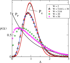
Figure 1: (Color online) The distribution $p(\Delta)$ for the 2D Ando model in the metallic, critical ($W=5.84$), and localized regime. The linear size of the system is $L=14$. The data are compared with the Wigner surmise $P_{4}(\Delta)$ and with the Poisson distribution $P_{P}(\Delta)$. While $p(\Delta)$ is very similar to the Wigner surmise in the metallic regime ($W=2$), it resembles the Poisson distribution when the disorder increases. However, for any disorder strength, $p(\Delta)$ decreases to zero when $\Delta\to 0$.

In the limit of strong disorder, $x_{1}\gg 1$, the typical conductance is given by the smallest parameter $x_{1}$ as $g\approx e^{-x_{1}}$. The parameter $x_{1}$ determines the localization length $\lambda$ as $x_{1}=2L/\lambda$ ($L\gg\lambda$). Thanks to this relation, the transport properties of strongly disordered system can be understood from the numerical analysis of relatively small samples, provided that $L\gg\lambda$.

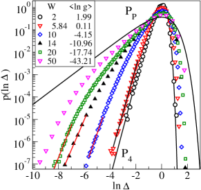
Figure 2: (Color online) The distribution $p(\ln\Delta)$ for the 2D Ando model. The linear size of the samples is $L=14$. The solid curves represent the Wigner $P_{4}$ and the Poisson $P_{P}$ distributions. With increasing disorder, the distribution of $p(\ln\Delta)$ changes. It is similar to Poissonian in the bulk, but for very small $\Delta$ we see the linear behavior $\ln p(\ln\Delta)\propto\ln\Delta$. The straight solid lines are fits for $W=5.84$, 10, 14, and 20 with slopes 4.789, 3.78, 3.0, and 3.3, respectively.

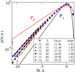
Figure 3: (Color online) The distribution $p(\ln\Delta)$ for a 2D orthogonal model with anisotropic hopping ($t_{xx^{\prime}}=0.9t_{zz^{\prime}}$). Two ensembles with different values of $L$ and $W$ but with the same value of $\langle\ln g\rangle$ possess the same distribution $p(\Delta)$. The Wigner surmise $P_{1}$ and the Poisson distribution $P_{P}$ are also plotted. Fits shown by straight lines confirm that $\ln p(\ln\Delta)\propto\ln\Delta$ with slopes given in the legend. Therefore, $p(\Delta)\sim\Delta$ when $\Delta\to 0$. The number of samples is $N_{\rm stat}=1.6\times 10^{9}$ for $L=20$ ($W=12$), and about $10^{8}$ else.

We analyze statistical ensembles of $N_{\rm stat}\sim 10^{8}$ square samplesFN (typical size is $L=14$) and collect the statistical distribution of the normalized difference. The results are displayed in Figs. 1-4 for the 2D Ando model and for the 2D orthogonal model. Fig. 1 exhibits the distribution $p(\Delta)$ for various strengths of the disorder. The data show that for small disorder ($W=2$) the distribution is very similar to the Wigner surmise. Although the form of the distribution changes when disorder increases, the decrease $p(\Delta)\to 0$ is noticeable even for $W=50$. The small-$\Delta$ behavior of the distribution is better visible in Fig. 2 which plots the distribution $p(\ln\Delta)$. Our numerical data for any disorder show that the distribution $p(\ln\Delta)$ becomes parallel to the Wigner surmise for very small $\Delta$. This proves that $\ln p(\ln\Delta)\sim(\beta+1)\ln\Delta$ and, consequently, $p(\Delta)\sim\Delta^{\beta}$ (Eq. (12)). However, the power-like behavior $p(\Delta)\sim\Delta^{\beta}$ is observed only for a very small part of the statistical ensemble. For instance, the linear behavior $p(\ln\Delta)\sim(\beta+1)\ln\Delta$ is observable only for $\ln\Delta<\ln\Delta_{m}=-4$ ($W=10$), $-7$ ($W=20$) (Fig. 2). The probability $p$ to find a system with such a small value of $\Delta$ decreases rapidly when the disorder increases: $p\sim 10^{-3}$ ($W=10$) but $p\sim 10^{-6}$ for $W=20$.

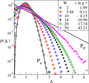
Figure 4: (Color online) The same as in Fig. 1 but on a logarithmic scale for various strength of the disorder and $L=14$. Solid lines are Wigner and Poisson distributions. For the localized regime ($W\geq 10$), the mean value of the logarithm of the conductance is given in the legend.

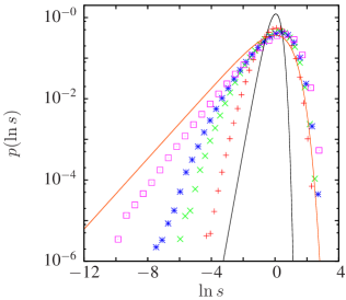
Figure 5: (Color online) The energy level statistics $p(\ln s)$ of a strongly disordered Ando model. In the limit of $s\to 0$, a clear $\sim s^{\beta+1}$ behavior is observed for $W=10$ from the comparison with the Wigner surmise $P_{4}$ for symplectic symmetry. With increasing $W$ the range where this agreement holds shifts to smaller $s$. The Poisson fit (upper solid line) is valid only for larger $s$. The system size is $L=20$ and the disorder strengths shown are $W=\mathrm{10}$ (+), 13 ($\times$), 15 ($\ast$), and 25 ($\Box$), respectively.

According to single parameter scaling theory,AALR the same change of the distribution function is expected when the size $L$ of the system increases while disorder is fixed. Owing to the necessity to analyze huge statistical ensembles, we did not study the size dependence of $p(\Delta)$ for the Ando model. However, we checked the $L$-dependence for 2D orthogonal systems (Fig. 3). Again, the distribution $p(\ln\Delta)$ follows Eq. (12) with $\beta=1$ provided that $\Delta$ is sufficiently small. Also, our data support the scaling idea: two distributions are similar if they correspond to systems with the same value of $\langle\ln g\rangle$.

To estimate the large-$\Delta$ form of the distribution, we plot in Fig. 4 $p(\Delta)$ for the Ando model and compare it with the Wigner distribution $P_{4}$ and the Poisson distribution. Again, our data confirm that $p(\Delta)$ is never identical with the Poisson distribution. For large values of $\Delta$ the distribution is $p(\Delta)\sim\exp(-c\Delta^{b})$ with exponent $b\approx 2$, at least in the limit of $\Delta\gg 1$.

The numerical investigation of the energy level statistics generated a similar result. For large disorder, $W>W_{c}\simeq 5.84$, the large-$s$ part of the level statistics $p(\ln s)$ is well described by the Poisson distribution as shown in Fig. 5. In the opposite limit $s\to 0$, a behavior close to the Wigner surmise $P_{4}$ is observed in which the range of the agreement is continuously diminishing with increasing disorder. For very large $W>20$, however, only the downturn can still be noticed. The eigenvalues have been calculated within an energy interval $-0.5\leq\varepsilon_{i}\leq 0.5$ by direct diagonalization of the respective $(2L)^{2}\times(2L)^{2}$ matrices with up to $3\times 10^{5}$ realizations. Additional calculations for larger system sizes corroborated the results shown here for $L=20$.

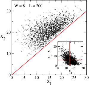
Figure 6: (Color online) Plot of parameters $x_{1}$ and $x_{2}$ for a statistical ensemble of $10^{4}$ samples. The size is $L=200$ and disorder $W=8$. The inset shows the value of the difference $x_{2}-x_{1}$ as a function of $x_{1}$. Solid lines mark mean values, $\langle x_{1}\rangle=14.09$ and $\langle x_{2}-x_{1}\rangle=6.08$. The data confirm the level repulsion since $x_{2}$ and $x_{1}$ never coincide. Note that small values of $\Delta$ are observed only in samples with relatively large value of $x_{1}>\langle x_{1}\rangle$. Such samples only marginally influence the mean conductance.

Our numerical data indicate that the generalized DMPKE fails to describe correctly the small-$\Delta$ behavior of $p(\Delta)$. Contrary to the expected behavior $p(\Delta)\propto\Delta^{\gamma}$, we observe for any disorder that $p(\Delta)\propto\Delta^{\beta}$. This restriction influences the statistical properties of the conductance only weakly since samples with small $\Delta$ represent only a very small part of the total statistical ensemble of the $N_{\rm stat}$ samples. Also, as shown in Fig. 6, samples with small $\Delta$ possess a large value of the smallest exponent $x_{1}>\langle x_{1}\rangle$, and consequently have also a small conductance. Therefore, their contribution to the conductance statistics is negligible. We expect that the GDMPKE gives a correct value of the mean $\ln g$ but its description of the small-$g$-tail of the distribution $p(\ln g)$ can eventually differ from numerical (experimental) data.

The aim of this paper was to verify that the physical symmetry of the model governs the small $\zeta$ behavior of the distribution $p(\zeta)$, where $\zeta$ denotes the normalized differences $\Delta=x_{2}-x_{1}/\langle x_{2}-x_{1}\rangle$ or, for the energy level statistics, the normalized difference of consecutive eigenvalues $s=|\varepsilon_{i+1}-\varepsilon_{i}|/\bar{s}$. This was done by a numerical study for the metallic and also in the strongly localized regime. Our results confirm that the generalized DMPK equation is not in contradiction with conclusions provided by random matrix theory.

We also showed that the distribution $p(\Delta)$ never corresponds entirely to the Poisson distribution, although $\gamma\to 0$. $p(\Delta)$ is not universal in the strongly disordered limit since $\gamma$ depends on the disorder. For small $\Delta$ we found a distribution $p(\Delta)\sim\Delta^{\beta}$ and in the limit of large $\Delta$ it behaves as $\exp(-c\Delta^{2})$. This observation is also consistent with the generalized DMPK equation. The Poisson distribution indicates that the two parameters, $x_{1}$ and $x_{2}$, are statistically independent. On the contrary, as discussed in previous work,M2000 ; MMW the statistical correlations survive for any disorder strength and are responsible for the non-Gaussian distribution of the logarithm of the conductance.

PM thanks the Grant Agency VEGA for financial support of the Project No. 0633/09.

References

- Muttalib and Klauder (1999) K. A. Muttalib and J. R. Klauder, Phys. Rev. Lett. 82, 4272 (1999).
- Muttalib and Gopar (2002) K. A. Muttalib and V. A. Gopar, Phys. Rev. B 66, 115318 (2002).
- Dorokhov (1982) O. N. Dorokhov, Solid State Communications 41, 431 (1982).
- Mello et al. (1988) P. A. Mello, P. Pereyra, and N. Kumar, Ann. Phys. (N.Y.) 181, 290 (1988).
- (5) P. A. Mello and N. Kumar, Quantum Transport in Mesoscopic Systems, Oxford Univ. Press (2004), Oxford, UK
- Economou and Soukoulis (1981) E. N. Economou and C. M. Soukoulis, Phys. Rev. Lett. 46, 618 (1981).
- Pichard (1991) J.-L. Pichard, in Quantum Coherence in Mesoscopic Systems, edited by B. Kramer (Plenum Press, New York, 1991), vol. 254 of Nato ASI, pp. 369–399.
- Altshuler and Shklovskii (1986) B. L. Altshuler and B. I. Shklovskii, Sov. Phys. JETP 64, 127 (1986).
- Altshuler et al. (1988) B. L. Altshuler, I. K. Zharekeshev, S. A. Kotochigova, and B. I. Shklovskii, Sov. Phys. JETP 67, 625 (1988).
- Shklovskii et al. (1993) B. I. Shklovskii, B. Shapiro, B. R. Sears, P. Lambrianides, and H. B. Shore, Phys. Rev. B 47, 11487 (1993).
- (11) A. M. S. Macedo and J. T. Chalker, Phys. Rev. B 46, 14985 (1992)
- (12) K. A. Muttalib, P. Markoš and P. Wölfle, Phys. Rev. B 72, 125317 (2005)
- (13) P. A. Mello, J. Phys. A 23, 4061 (1990)
- (14) P. Markoš and B. Kramer, Ann. Phys. 2, 339 (1993)
- Schweitzer and Kh. Zharekeshev (1997) L. Schweitzer and I. Kh. Zharekeshev, J. Phys.: Condens. Matter 9, L441 (1997).
- Batsch et al. (1998) M. Batsch, L. Schweitzer, and B. Kramer, Physica B 249-251, 792 (1998).
- Potempa and Schweitzer (2002) H. Potempa and L. Schweitzer, Phys. Rev. B 65, 201105(R) (2002).
- Markoš and Schweitzer (2006) P. Markoš and L. Schweitzer, J. Phys. A 39, 3221 (2006).
- (19) Although DMPKE was derived for quasi-one dimensional systems, there is strong numerical evidence that its predictions are applicable also for 2D and 3D systemsMMW
- (20) E. Abrahams, P. W. Anderson, D. C. Licciardello, T. V. Ramakrishnan, Phys. Rev. Lett. 42, 673 (1979).
- (21) P. Markoš, Phys. Rev. B 65, 104207 (2002).