NGC 1300 Dynamics: III. Orbital analysis

Abstract

We present the orbital analysis of four response models, that succeed in reproducing morphological features of NGC 1300. Two of them assume a planar (2D) geometry with $\Omega_{p}$=22 and 16 km s^-1 kpc^-1 respectively. The two others assume a cylindrical (thick) disc and rotate with the same pattern speeds as the 2D models. These response models reproduce most successfully main morphological features of NGC 1300 among a large number of models, as became evident in a previous study. Our main result is the discovery of three new dynamical mechanisms that can support structures in a barred-spiral grand design system. These mechanisms are presented in characteristic cases, where these dynamical phenomena take place. They refer firstly to the support of a strong bar, of ansae type, almost solely by chaotic orbits, then to the support of spirals by chaotic orbits that for a certain number of pattern revolutions follow an n:1 (n=7,8) morphology, and finally to the support of spiral arms by a combination of orbits trapped around L_4,5 and sticky chaotic orbits with the same Jacobi constant. We have encountered these dynamical phenomena in a large fraction of the cases we studied as we varied the parameters of our general models, without forcing in some way their appearance. This suggests that they could be responsible for the observed morphologies of many barred-spiral galaxies. Comparing our response models among themselves we find that the NGC 1300 morphology is best described by a thick disc model for the bar region and a 2D disc model for the spirals, with both components rotating with the same pattern speed $\Omega_{p}$=16 km s^-1 kpc^-1 ​. In such a case, the whole structure is included inside the corotation of the system. The bar is supported mainly by regular orbits, while the spirals are supported by chaotic orbits.

1 Introduction

In Kalapotharakos et al. (2010a) (hereafter PI) we have proposed three general models for the potential of the barred-spiral galaxy NGC 1300, which reflect three different geometries of the system. In the extensive study presented in Kalapotharakos et al. (2010b) (hereafter PII) we have found several response models that reproduce at an acceptable degree morphological features of NGC 1300. Varying the pattern speed in models with all three assumed geometries, we concluded that the main features of NGC 1300 were better reproduced in models clustered around two $\Omega_{p}$ values, namely 16 and 22 km s^-1 kpc^-1 ​. Taking into account the index used for the comparison of the models (PII) and the empirical by eye assessment of the resulting morphologies, we sorted out the following four “best” cases. We remind that there was no single model reproducing all the features in an optimal way):

1. Model 1: A 2D (Case A in PI) model, rotating with $\Omega_{p}$=22 km s^-1 kpc^-1 ​. The main success of this model is the reproduction of the bar morphology.

2. Model 2: A 2D (Case A in PI) model, rotating with $\Omega_{p}$=16 km s^-1 kpc^-1 ​. The main success of this model is the reproduction of the spiral morphology.

3. Model 3: A thick disc model of cylindrical geometry (Case B in PI), rotating also with $\Omega_{p}$=16 km s^-1 kpc^-1 ​. The main success of this model is a nice reproduction of the bar’s morphology. Its response at the spiral region succeeds in giving the density maxima of the model roughly at about the same area occupied by the spiral arms of the galaxy. However, the response at the spiral region of the model forms a spurious ring structure.

4. Model 4: Another thick disc model of cylindrical geometry (Case B in PI), rotating this time with $\Omega_{p}$=22 km s^-1 kpc^-1 ​ (as Model 1), develops a spiral structure that is worth to be presented as a separate model, since the spiral arms are formed through a different dynamical mechanism than that in Model 2.

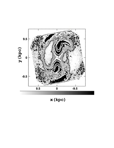
Figure 1: The morphology of the barred-spiral perturbation in NGC 1300. The deprojected K-band image has been divided by the mean surface brightness at each radius. The original image is flipped in x and rotated clockwise by $4\pi/9$ to better compare with the orbital models. Isocontours of a smoothed K-band image are overplotted to emphasize the morphological details.

We will follow the detailed orbital analysis of these four models in the subsequent sections. Nevertheless, we want to underline, that the goal of our paper is to present the dynamical mechanisms behind the observed structures. Besides the morphological similarities between response models and NGC 1300 we have chosen the four cases, because they represent different dynamical mechanisms leading to the formation of the bar and the spirals. This gives us the opportunity to compare different possible dynamics that lead to the support of similar structures in the galactic disc. In that sense the four models should be considered as typical cases for the description of different dynamics behind them.

A characteristic difference of the model potential from other barred-spiral models we find in the relevant literature (Kaufmann & Contopoulos, 1996; Patsis et al., 1997; Harsoula & Kalapotharakos, 2009; Patsis et al., 2009) is its asymmetry. As we can see in the near-infrared image of NGC 1300 (fig. 3b in PI), the two spiral arms have different morphologies. Both arms emerge out of the ends of the bar as a continuation of an ansae structure. However, the ends of the ansae, i.e. the regions where the spiral arms begin, are not at equal distances from the center of the galaxy. The bar itself is asymmetric with its lower end being closer to the center of the galaxy.

Both spiral arms are strong at their beginning, close to the ends of the bar, in the near-infrared, even after correcting for star formation (PI). Notwithstanding, they weaken as we move azimuthally away from the bar. In order to clearly observe the exact shape of the spiral arms we divide in Fig. 1 the deprojected K-band image with the mean surface brightness at each radius. The arm at the left side of Fig. 1 could be considered as continuous, although its surface brightness varies azimuthally and has a clear minimum at a height corresponding roughly to the middle of the bar. However, the right arm in Fig. 1 is conspicuously discontinuous and has a second strong part at the opposite end of the bar than the one it emerges from. All these asymmetries are taken into account in the potential we use (PI) and thus in our orbital calculations. We study a fully asymmetric dynamical behaviour. We note that the spiral arms have in the K-band relative sharp features. This supports a quasi-stable character, since transient features, due to different wave packages, are more likely to be smooth.

In order to facilitate our calculations and the adaption of the potential models to our computer programs, we have flipped the potential around the central column and then we have rotated it by $4\pi/9$ counterclockwise. This allows us to study models in which the sense of rotation of the galaxy is counterclockwise and the major axis of the bar is close to the y-axis of our Cartesian coordinate system. All figures in the present paper have this orientation.

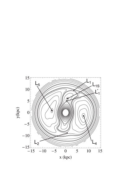
Figure 2: The effective potential isocontours for our 2D Model 1 with $\Omega_{p}=22$ km s^-1 kpc^-1 ​. We have one stable (L_1S) and five unstable (L₄, L₅, L₁, L${}_{1^{\prime}}$, L₂) Lagrangian points indicated with arrows.

Equations of motion are derived from the Hamiltonian

$$H\equiv\frac{1}{2}\left(\dot{x}^{2}+\dot{y}^{2}\right)+\Phi(x,y)-\frac{1}{2}\Omega_{p}^{2}(x^{2}+y^{2})=E_{J},$$ (1)

where $(x,y)$ are the coordinates in the Cartesian frame of reference as defined above, rotating with angular velocity $\Omega_{p}$. $\Phi(x,y)$ is the potential in Cartesian coordinates and can be anyone of the three models presented in PI. E_J is the numerical value of the Jacobi constant and dots denote time derivatives.

As we have seen in PII the range of $\Omega_{p}$ values for which a certain similarity between response models and galaxy could be traced was $12<\Omega_{p}<26$ km s^-1 kpc^-1 ​. Beyond that range the resemblance of the response models with the morphology of the galaxy was visibly problematic. So we did not follow the evolution of the responses in models with pattern speeds out of this range.

2 Model 1

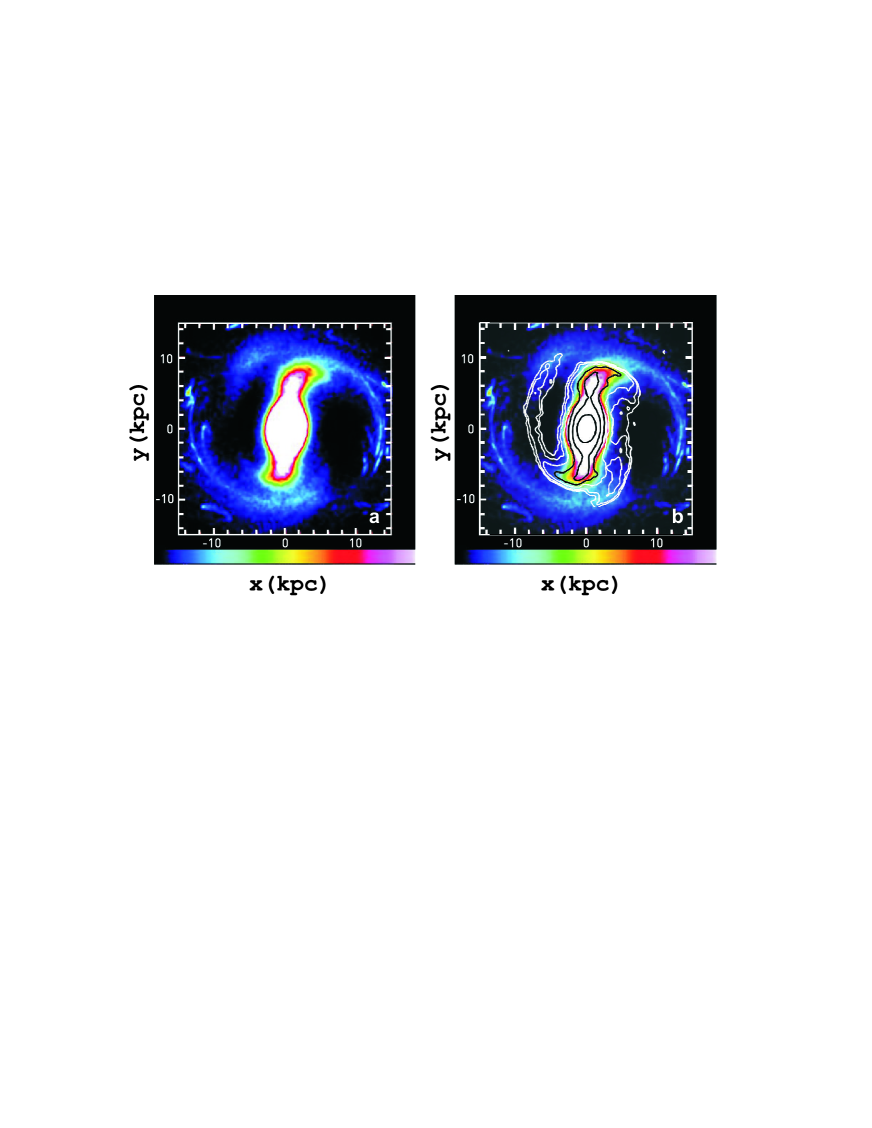
Figure 3: Color-scaled density response of Model 1 (2D, $\Omega_{p}$ = 22 km s^-1 kpc^-1 ). (a) We observe the appearance of a typical grand-design barred-spiral morphology. (b) Characteristic isocontours of the deprojected K-band image of the galaxy, different than those given in Fig. 1, are overplotted on the response model. Model 1 has a bar with a morphology similar to the bar of NGC 1300, but its spirals are clearly more open than the spirals of the galaxy.

For $\Omega_{p}>21$ km s^-1 kpc^-1 the isocontours of the effective potentials have a remarkable shape. This is shown in Fig. 2, for our Model 1 ($\Omega_{p}=22$ km s^-1 kpc^-1 ). Besides the stable Lagrangian point at the center of the galaxy (not indicated on Fig. 2) and the usual equilibrium points at the sides of the bar (L₄, L₅), there appears one more stable Lagrangian point (L_1S), as a result of the complicated “landscape” at the upper part of the bar. At this region we have two unstable Lagrangian points (L₁ and L${}_{1}^{\prime}$). L${}_{1}^{\prime}$ appears close to the middle of the upper semi-major axis of the bar, at a lower E_J value ($-170759$) than that of L₁ ($-167409$). Thus, between the unstable points L${}_{1}^{\prime}$ and L₁ appears L_1S, which is stable. Nevertheless, close to the lower end of the bar, we have only one unstable Lagrangian point, L₂, as usual (Fig. 2). Due to the asymmetry of the potential, L₂ has a larger E_J value ($-166797$) than that of L₁. We also note, that L₄ and L₅ in this case are unstable (see PI). However, as we will see below, the associated simple periodic orbits are stable in large intervals of the Jacobi constant.

To our knowledge it is the first time that a systematic orbital analysis is done in a galactic effective potential with more than two equilibrium points roughly along the major axis of the bar.

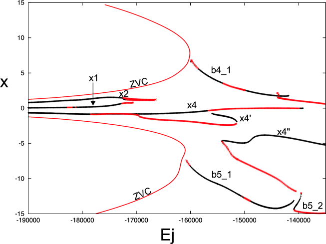
Figure 4: ($x$,E_J ) characteristics of the main families of periodic orbits of Model 1. The curves designated with “ZVC” correspond to the two branches of the zero velocity curve in this diagram. Black parts on the characteristic curves of the families indicate stability, while grey (red in the online version) instability. The maxima of the ZVC’s are near L₄, L₅.

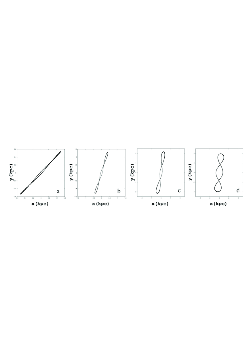
Figure 5: Stable x1 orbits for Model 1 . (a) E_J = $-210000$, (b) E_J = $-190000$ (c) E_J = $-180098$ (d) E_J = $-170677.78$. The x1 orbit in (d) is the longest x1 along the major axis of the bar found in this model. The sizes of the frames are not equal in the four panels.

The response of Model 1 is given in Fig. 3. It is a density map of the stellar response. In this and all subsequent density maps of our response models the colored bar below the figure represents increasing density from left to right. Information about the initial set up and the initial conditions and other details about the construction of the models are given in PII. Here, with Fig. 3a we want to show that our 2D model rotating with $\Omega_{p}$ = 22 km s^-1 kpc^-1 gets a barred-spiral morphology with spiral arms emerging close to the ends of the bar. The response morphology is typical of grand-design barred-spiral galaxies. The bar is a typical ansae-type bar, as the bar of NGC 1300, while the spiral arms are rather symmetric, and extend azimuthally roughly over an angle of $\pi/2$, beginning at the Lagrangian points L₁ and L₂ of the effective potential (cf. with Fig. 2).

In such a model it is tricky to point to a single $R_{CR}/R_{b}$ ratio (see figure 2 of PII). On one hand the ends of the bar are not at equal distances from the center of the galaxy. Then, $R_{b}$, the bar radius, is not unambiguously defined. On the other hand all Lagrangian points are found within a ring of width about 5 kpc and one cannot speak about a single corotation radius $R_{CR}$. By considering the upper length of the bar and the L₁ radius we find a $R_{CR}/R_{b}$=1.16, while we have $R_{CR}/R_{b}$=1.11 if we consider the lower length of the bar and the L₂ radius.

In Fig. 3b we overplot on the response Model 1, characteristic isophotes of the deprojected K-band image of the galaxy. The ansae-type response bar matches the size of the NGC 1300 bar both in length and width. The location of the ansae are in agreement with the location of the ansae of the bar of the galaxy. On the other hand the developed spiral structure of the model has no relation with the asymmetric spiral pattern we are trying to reproduce (Fig. 3b). In order to understand the orbital content behind the observed structures, we firstly investigate the families of periodic orbits existing in Model 1. We want to check to what extent the observed structures are built by regular orbits trapped around stable periodic orbits used as building blocks. The standard way to build a bar in a rotating galactic potential is with regular orbits trapped around the stable x1 orbits (Contopoulos, 1980).

2.1 Families of periodic orbits

The ($x$, E_J ) characteristic for Model 1 is given in Fig. 4. The $\dot{x}$ initial condition of the orbits, is not taken into account in this diagram. Also we note that the L₄, L₅ Lagrangian points are not exactly on the x-axis of the system. Thus, the upper and lower local maxima of the zero velocity curves (ZVC) at E_J $\lessapprox-160000$ do no correspond to L₄ and L₅ respectively. In Fig. 4 we observe that the main part of the central family, x1, stops before E_J $=-170000$, while the other known family in rotating barred potentials, x2, together with a family bifurcated from it, reach a Jacobi constant value close to $-165000$. Our system has a Central Mass Concentration (CMC) term (PI), due to which both characteristics of x1 and x2 join at the center of the system (not included in Fig. 4). The two families evolve in parallel as the value of the Jacobi constant increases with x2 having always larger $x$ initial conditions than x1. Both families have large stable parts, which are drawn black, while the unstable parts along the characteristic curves are plotted in grey. For the estimation of the stability of the periodic orbits we calculate their Hénon index (Hénon, 1965). The morphological evolution of the central family, which provides Model 1 with stable orbits extended along the major axis of the bar, resembles that of the propeller orbits presented by Kaufmann & Patsis (2005). They have loops already for small values of the Jacobi constant.

Fig. 5 shows this morphological evolution of x1. From (a) to (d) we plot stable representatives of this family for E_J = $-210000$ (a), E_J = $-190000$ (b), E_J = $-180098$ (c) and E_J = $-170677.78$ (d). The orbit given in Fig. 5d is the longest stable x1. The x2 orbits, extending in this model in the same Jacobi constant interval as the x1 family, are asymmetric. Two of them are given in Fig. 6 and both of them are stable. The black one is at E_J ​=$-180000$, while the grey one, for E_J =$-172572.1$ is the last stable x2 of the system. We observe that both of them are elongated along the minor axis of the bar as expected, they are asymmetric and their projections on the x-axis do not extend to radii larger than 2.5 kpc. Thus, they are embedded in the central region of Model 1 in Fig. 3. For Figs. 6 and all other figures with orbits in this paper the axes are considered as x, y Cartesian coordinates and the units on the axes are in kpc.

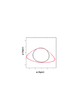
Figure 6: Asymmetric, stable x2 periodic orbits in Model 1 for E_J =$-180000$ (black) and for E_J =$-172572.1$ (grey - red in online version).

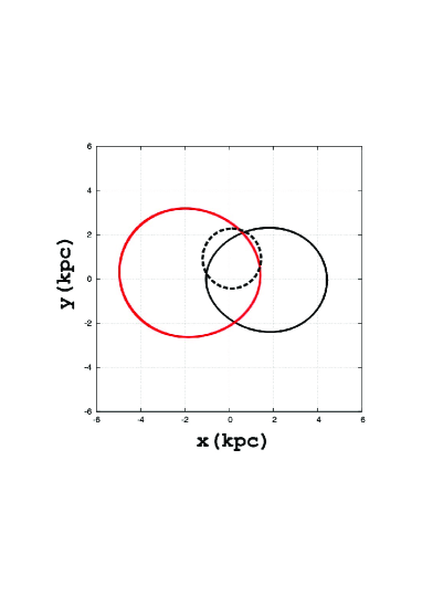
Figure 7: Asymmetric with respect to the center of the system x4-like orbits. x4 at E_J =$-170000$ (dashed); x4^′, a bifurcation of x4, at E_J =$-154352.2$ (black); and x4^′′ at E_J =$-150000$ (grey - red in the online version)

.

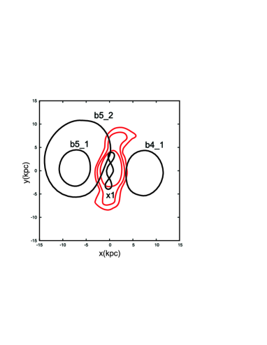
Figure 8: Characteristic stable orbits of x1 (longest along the bar in the system) and of the families b4_1, b5_1 and b5_2, drawn with black color, together with isodensity contours of Model 1 (grey curves - red in the online version). These orbits can hardly support the developed morphology of Model 1.

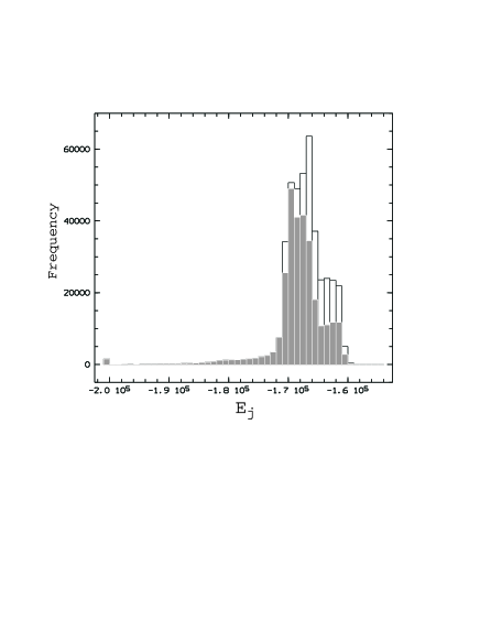
Figure 9: Energy statistics for the particles of Model 1 depicted in Fig. 3. Black refers to the total number of particles of the model, while the overplotted grey histogram gives the statistics at $r<9.2$ kpc, practically the statistics of the bar particles.

Another set of periodic orbits that exist over large Jacobi constant intervals in Fig. 4 belong to x4 and x4-like families. They are counterrotating orbits designated on Fig. 4 with x4, x4^′ and x4^′′. All of them are displaced with respect to the center of the system. Characteristic representatives of these families are given in Fig. 7. A grid is included in the figure for better understanding the described asymmetries. The last main families of stable periodic orbits in the system are families of banana-like orbits around the Lagrangian points L₄ and L₅. The branches of the characteristic curves belonging to them are denoted with b4_1, b5_1 and b5_2 in Fig. 4. In order to have an overview of the morphological features of Model 1 that could be supported by stable periodic orbits, through trapping of regular orbits around them, we plot in Fig. 8 orbits of the families x1 (E_J = $-170677.78$), b4_1 (E_J = $-154102$), b5_1 (E_J = $-155000$) and b5_2 (E_J = $-140398$), black curves, together with isodensity contours of the bar of Model 1 (grey curves). The plotted x1 orbit is the one given in Fig. 5d, i.e. the longest stable orbit of this family. It is clear that in this case stable x1 orbits can support only the central bar region, as their projections on the major axis of the bar cannot exceed radii of 4 kpc maximum. Thus, the loops of the x1 orbits are not related with the ansae of the response model. It is evident from Fig. 8, that the building blocks of the bar of Model 1 are not the stable orbits of the x1 family. Moreover, comparison of Fig. 8 with Fig. 3 clearly shows that the superposition of stable orbits of the banana-like families can hardly support the open spiral pattern of the response model, which in any case is not in good agreement with the spiral structure of NGC 1300. In conclusion, the grand design barred-spiral structure of Model 1 is rather unlikely to be shaped due to the usual mechanism that uses stable periodic orbits as building blocks. The question about what shapes the observed morphology remains.

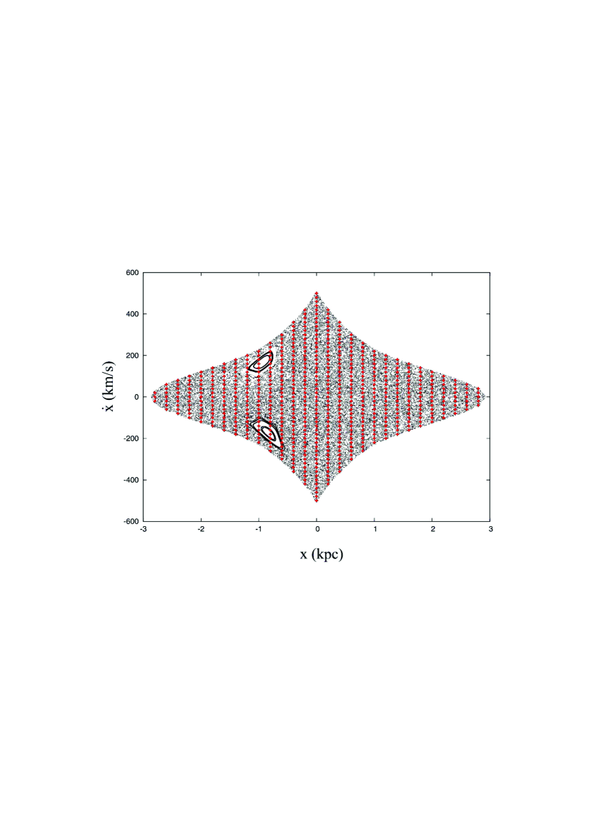
Figure 10: The (x,ẋ) surface of section at E_J = $-1.7\times 10^{5}$ for Model 1. The overplotted red points indicate 587 initial conditions that have been integrated for time corresponding to 7 pattern rotations. The morphology of the individual trajectories has been examined in the text.

The next step that will help us understand the orbits of the particles in the model is to study the statistics of their Jacobi constants at several regions. In the present case it is rather easy to roughly separate the particles on the bar from the particles on the spiral arms, because the spirals of the model are open and the region between spiral arms and bar is quite empty. Essentially bar particles are those with $r<9.2$ kpc, while the vast majority of the particles with $r>9.2$ kpc are on the spiral arms.

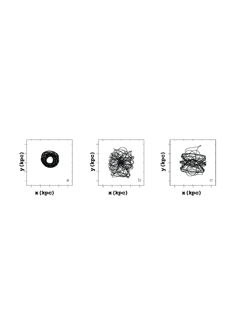
Figure 11: Orbits for Model 1 at E_J = $-1.7\times 10^{5}$. (a) A sticky chaotic orbit close to x4, (b) a chaotic orbit staying inside a 4 kpc radius and (c) a chaotic orbit that for a certain time fraction follows a x2 flow.

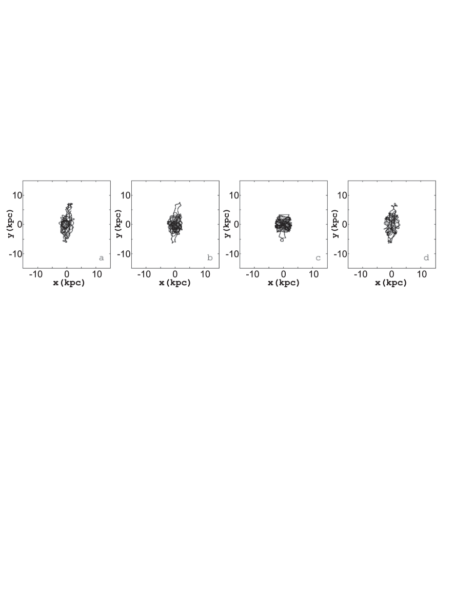
Figure 12: Chaotic orbits in Model 1 with E_J =$-170000$, which support the ansae bar morphology. From (a) to (d) the initial $(x,\dot{x})$ conditions of the orbits are $(-0.2,-360)$, $(0.4,-320)$, $(1.3,-200)$ and $(0.8,-100)$.

The histogram with the Jacobi constant statistics for Model 1 is given in Fig. 9. With grey is given the statistics of the particles at $r<9.2$ kpc, while the black bars that come on top of the grey ones refer to the total number of particles and appear at higher levels beyond a certain value of the Jacobi constant. We observe that we do not have any particles for E_J $>-1.58\times 10^{5}$. By looking at Fig. 4 we realize that no particles are trapped around stable banana-like periodic orbits. Only small segments of the characteristics of b4_1 and b5_1 exist at E_J $<-1.58\times 10^{5}$. Especially close to the upper local maximum of the ZVC, close to L₄, there are only unstable b4_1 periodic orbits. The interval E_J $<-1.58\times 10^{5}$ includes only a small segment of stable periodic orbits belonging to the b5_1 banana-like family. Practically the characteristics at the right part of Fig. 4 belong to families that are not related with the model. The grey histogram, that refers to the bar particles, shows that these particles have Jacobi constants in the interval $-1.71\times 10^{5}<$ E_J $<-1.65\times 10^{5}$, with a peak at $-1.7\times 10^{5}<$ E_J $<-1.69\times 10^{5}$. What is the orbital behaviour at these Jacobi constants? The range of the Jacobi constants roughly covers the region between the last x1 orbits and the local maxima of the ZVC close to the L₄ and L₅ points (Fig. 4). Knowing the range of E_J ’s that contributes mostly to the orbital content of the bar, we investigate the surfaces of section at these Jacobi constants. The (x,ẋ) surface of section for E_J = $-1.7\times 10^{5}$, close to the mode of the distribution, is given in Fig. 10. There are depicted about $5\times 10^{4}$ consequents with black points. The only two conspicuous islands of stability belong to the asymmetric x4 retrograde orbits. The one with negative velocity is like the dashed orbit in Fig. 7, while the other one, with positive velocity, is its symmetric with respect to the y=0 axis. Apart from these two islands of stability the rest of the surfaces of section is dominated by Chaos. We know however, that at this E_J we encounter most particles that contribute to the bar structure.

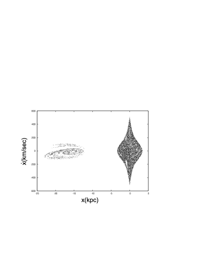
Figure 13: The (x,ẋ) surface of section for E_J =$-1.67\times 10^{5}$ in Model 1.

The chaotic sea can be in principle generated by a single chaotic orbit, if we integrate it for a long time. However, starting with different initial conditions and by integrating for relatively short times we do not obtain necessarily similar orbital morphologies. Integrating for finite time intervals a large number of initial conditions we simulate the situation of following the trajectories of individual particles on the galactic disc, and this allows us to understand whether they support a specific morphology within this time interval. The red symbols overplotted on the surface of section indicate 587 initial conditions on the (x,ẋ) surface of section in Fig. 10, that have been integrated for time corresponding to 7 pattern rotations. We will refer to all of the resulting trajectories also as “orbits”, despite the fact that the chaotic orbit is essentially one. The supported morphologies we found were quite distinct, and this allowed us to proceed to a crude by eye classification as follows:

Around 7% of the trajectories were related with the x4 retrograde family, being either regular quasi-periodic orbits trapped around them, or related sticky chaotic orbits. A typical orbit of this kind is given in Fig. 11a. Another 40% of the integrated trajectories were chaotic, staying in the inner bar region without ever exceeding a radius r=4 kpc. They were essentially supporting the part of the bar without the ansae. Such an orbit is presented in Fig. 11b. Only 1% of the chaotic orbits could be associated with x2-like orbits (Fig. 11c, cf. with Fig. 6). The remaining 52% of the integrated initial conditions belong to orbits in the chaotic sea, which share a common feature. These particles, after spending part of the integration time in the central bar region as in Fig. 11b, they visit the immediate neighborhood above and below the central part contributing to the formation and support of the ansae. Such orbits are presented in Fig. 12. We note that L${}_{1}^{\prime}$ appears at E_J =$-170759$, very close to the E_J value of the surface of section we study, indicating that the appearance of this type of orbits is associated with the presence of the stable and unstable manifolds of the unstable L${}_{1}^{\prime}$ equilibrium point. This type of chaotic orbits give the strong ansae type morphology of the bar of the response Model 1.

The other morphological feature, that characterizes Model 1, are its open spirals (Fig. 3). Despite the fact, that they do not match the NGC 1300 spirals, they are a strong feature of its grand-design morphology. They consist of particles at $r>9.2$ kpc. As we can conclude from Fig. 9 the mode, the value that occurs most frequently in the distribution of these particles, is found for $-1.68\times 10^{5}<$ E_J $<-1.66\times 10^{5}$. In order to find the orbital content of the model spirals we follow the same procedure. The (x,ẋ) surface of section for E_J =$-1.67\times 10^{5}$ is presented in Fig. 13. Being closer to the local maxima of the ZVC (Fig. 4) there appears in the diagram also a region to the left of the central area of the surface of section. At the central region the only conspicuous islands of stability are again those belonging to x4, as in the previous case we studied at E_J =$-1.7\times 10^{5}$.

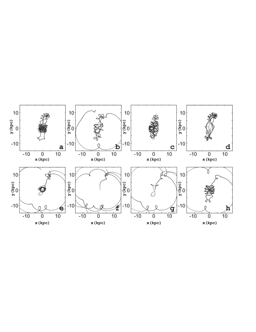
Figure 14: Chaotic orbits at E_J =$-1.67\times 10^{5}$ in Model 1. 63% of the initial conditions we integrated support a bar morphology with ansae, while 26% contribute to the formation of the spiral structure of the model. From (a) to (h) the initial $(x,\dot{x})$ conditions of the orbits are: $(-0.4,-360)$, $(0.2,-360)$, ($0.6,-280)$, ($-1.8,-160$), ($-1.4,-160$), ($1.2,40)$, ($0.2,200$), ($0.6,240$).

We have integrated again a large number of initial conditions for a time equal to 7 pattern rotations. In this case the number of orbits that support a bar with ansae increased to 63%, while an additional 26% abandon the bar region and by going through the L₁ location visit the area of the disc and the spirals. Typical orbits of the kind we describe can be observed in Fig. 14. The mechanism that shapes the open spirals of Model 1 is based on the presence of the family generated at the unstable Lagrangian point L₁, which has E_J =$-167409$. For a Jacobi constant just greater than it, at E_J =$-167000$, which is the Jacobi constant of the surface of section we study, the unstable periodic orbit associated with the open spiral pattern already exist. The chaotic sea is structured by the presence of the manifolds of this unstable periodic orbits. For this particular response model, the mechanism that builds its spiral arms is the one valid also for the spirals of NGC 4314 (Patsis, 2006). This mechanism, as in the case of NGC 4314, creates spirals with a strong part, that reaches azimuthally angles up to $\pi/2$ starting from the ends of the bar. Details about how chaotic spirals can be formed this way can be found in Voglis et al. (2006), Romero-Gomez et al. (2006), Voglis et al. (2006), Tsoutsis et al. (2009), Contopoulos (2009) (see also articles by the same authors in Contopoulos & Patsis (2009) and references therein). Our analysis shows however, that the spirals of NGC 1300 cannot be related with this mechanism. Thus, we continue the investigation of our response models in order to find a better explanation of the dynamical origin of the NGC 1300 spirals. We remind though, that the Model 1 bar reproduces in a satisfactory way the bar of NGC 1300.

3 Model 2

In PII we have seen that by lowering the pattern speed of the system in the 2D case to $\Omega_{p}=16$ km s^-1 kpc^-1 we obtained an excellent matching of the location of the spirals between model and galaxy. This case is our Model 2 of the present paper. We summarize its morphology with the help of Fig. 15. There are three main successes of Model 2 in its comparison with the NGC 1300 spirals: (i) the abrupt break of the upper arm, just after it emerges from the upper end of the bar. This is indicated in Fig. 15a with an arrow labeled “A”. (ii) the spiral fragment at the lower right side of the bar. An arrow labeled “B” points in Fig. 15a to this feature. (iii) the location and the pitch angle of the rather continuous left arm, indicated with the arrow labeled “C”. The overplotted on the model isophotes of the deprojected K-band image, show clearly the agreement of these features (Fig. 15b). This time the spiral structure is modeled at a very satisfactory level. However, the only feature of the bar that agrees with the NGC 1300 bar is its size. The model bar is thicker than the one of the galaxy and has only a weak ansae character.

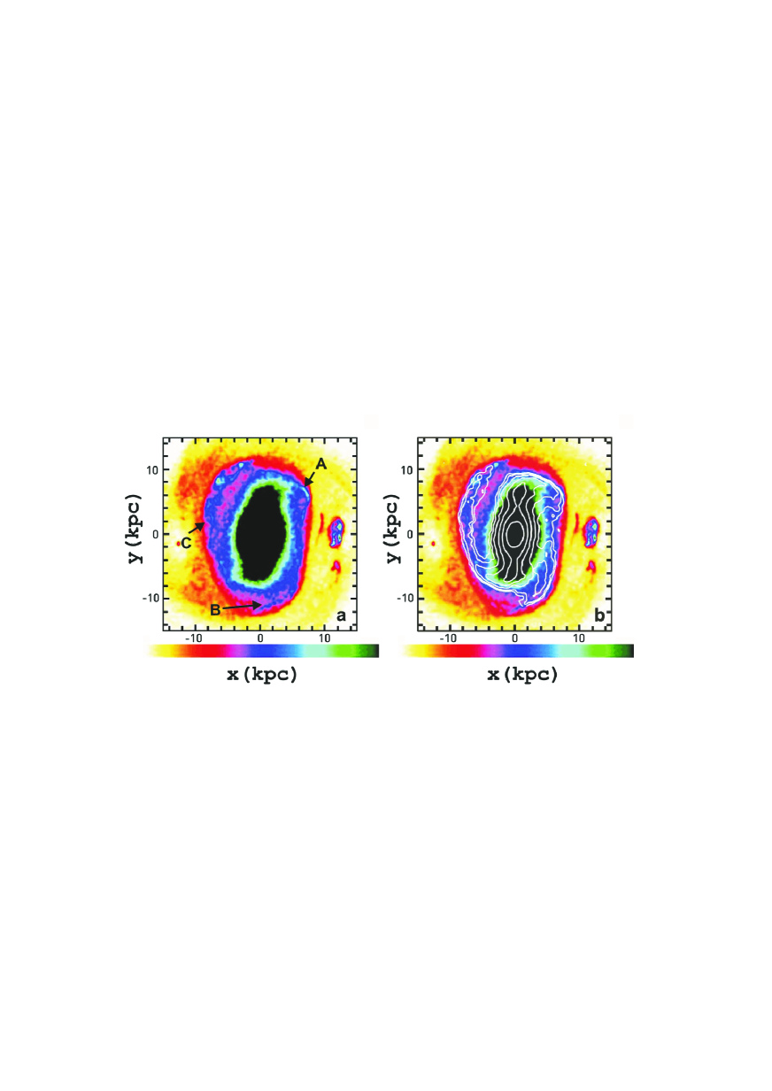
Figure 15: The colored-scaled density response of Model 2 (2D with $\Omega_{p}=16$ km s^-1 kpc^-1 ). In (a) we point with arrows to the three morphological features that resemble the corresponding structures of NGC 1300. In (b) we overplot on the model isophotes of the deprojected K-band image of NGC 1300, that show the level of agreement of the spiral morphology between model and galaxy.

Particularly interesting is the comparison of the effective potential isocontours (Fig. 16) with the resulting response model. Now, for $\Omega_{p}=16$ km s^-1 kpc^-1 , the Lagrangian points have moved to larger distances from the center. We have the usual two stable L₄ and L₅ equilibrium points (at approximately $-149690$ and $-150300$) and the two unstable L₁ and L₂ at $-152960$ and $-153020$ respectively. Besides them there is a third unstable equilibrium point, L${}^{\prime}{{}_{1}}$, at $\approx(-8,10)$. As a consequence, there is one more equilibrium point, L${}^{\prime\prime}{{}_{1}}$, between L₁ and L${}^{\prime}{{}_{1}}$, which in this case is unstable. All Lagrangian points appear beyond the end of the barred-spiral morphology of the response model altogether. Contrarily to Model 1, all the Lagrangian points in Model 2 are within a relative narrow ring of width about 1.8 kpc. However, the $R_{CR}/R_{b}$ ratios we find deviate more among themselves. By considering the upper length of the bar and the L₁ radius we find this time $R_{CR}/R_{b}$=1.44, while we have $R_{CR}/R_{b}$=1.68 if we consider the lower side of the bar and the L₂ radius.

We underline the presence of an isocontour in the effective potential, which we have drawn with a thicker line and to which we point with a thick white arrow. There is a striking similarity between the shape and the location of this isocontour in Fig. 16 and the border of the red region that surrounds the barred-spiral structure of the response Model 2 in Fig. 15. We discuss the role of this isophote for the dynamics of Model 2 in the following paragraphs.

The characteristics of the main families of periodic orbits in an (E_J , $x$) diagram, similar to the one presented in Fig. 4 for Model 1, is given in Fig. 17. The evolution of the x1, x2 families is similar to that of Model 1, but the Jacobi constant interval between the last stable x1 and the corotation region has increased significantly. Between them we have calculated segments of characteristics belonging to families with asymmetric morphologies we have classified as 4/1, 7/1 and 8/1. We also note the presence of segments of several 3/1 type families close to the largest Jacobi constants, where we still encounter x1 and x2 orbits. At all Jacobi constants in Fig. 17 we have always orbits belonging to x4 and its bifurcations. It is beyond the scope of the present paper to study the interconnections between the various families.

This time we have found periodic orbits extended roughly along the major axis of the system, which could contribute to the bar structure. In Fig. 18 we present some of them independently of their stability. (a) The longest stable x1 orbit at E_J = $-166579.83$. It has loops that now reach distances about 5 kpc from the center, (b) two 3/1 orbits at $-164476.07$ (dark grey) and $-163642.8$ (light grey), that are close to symmetric with respect to the y-axis and together can be considered as bar supporting, (c) a 4/1 orbit from the tiny stable part of the characteristic of this family at E_J =$-160018.42$ and finally at (d) the 4/1 representative at E_J =$-153480$.

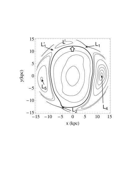
Figure 16: The effective potential isocontours for our Model 2 with $\Omega_{p}=16$ km s^-1 kpc^-1 ​. We have two stable (L₄, L₅) and four unstable (L₁, L${}_{1}^{\prime}$, L${}_{1}^{\prime\prime}$, L₂) Lagrangian points indicated with black arrows. The white thick arrow points to an isocontour, that surrounds the bar-spiral morphology.

We also give the morphology of the two families above the 4/1, at larger $x$. In (a) a stable 8/1 (E_J =$-154280.23$) and in (b) an unstable 7/1 (E_J =$-155046.68$) (Fig. 19). In order to trace the orbits of the particles that successfully reproduce the spiral structure of NGC 1300 in Model 2, we follow the same procedure as in Model 1. We isolate an area around the bar of the response model, which includes the spiral arms and we calculate the Jacobi constants of the particles in this area. The histogram with the Jacobi constant statistics at this region is given in Fig. 20. The histogram shows that the peak happens at the bin $-154000<$ E_J $<-153000$, while practically the Jacobi constants of all particles are $-156000<$ E_J $<-150000$. Most particles on the spirals of Model 2 have these E_J values. By looking at Fig.  17 we realize that at this region exist the 7/1 and 8/1 families, the “4/1” family with double multiplicity, as well as a segment of the 4/1 characteristic. Only for the 8/1 family the Hénon index is $|\alpha|<1$ (black segments in Fig. 17. This analysis shows that whatever the dynamical mechanism behind the appearance of the spiral structure is, it is related with particles on trajectories inside corotation.

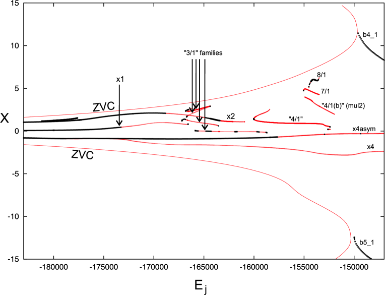
Figure 17: The characteristics of the main families in Model 2 (2D with $\Omega_{p}=16$ km s^-1 kpc^-1 ). We note the presence of the 4/1, 7/1 and 8/1 families at Jacobi constants $-160000\succapprox$ E_J $\succapprox-150000$. Black segments of the characteristics indicate stability, while grey (red in the online version)

instability. The maxima of the ZVC’s are near L₄, L₅.

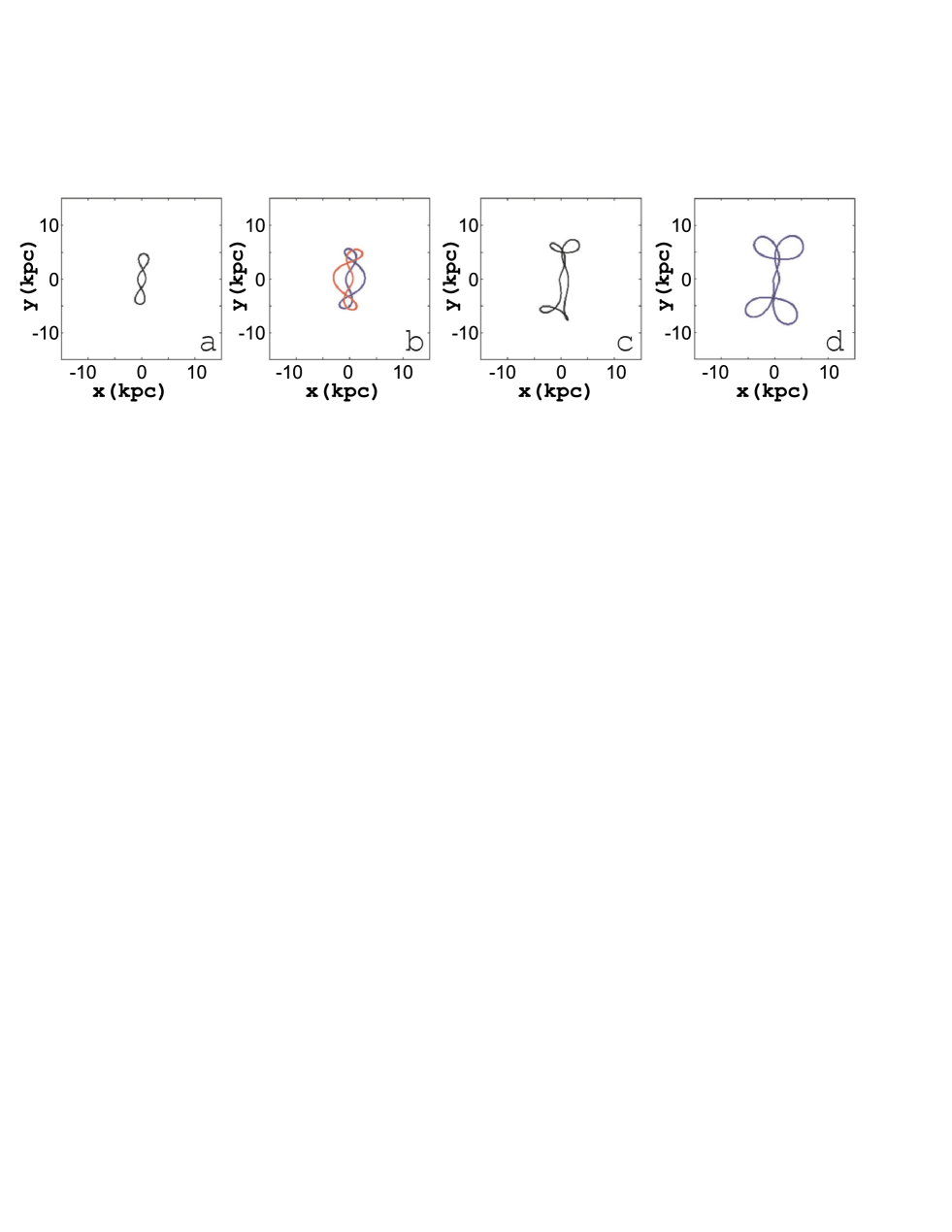
Figure 18: Periodic orbits in Model 2, that are elongated along the major axis of the bar. The orbits in (a), (b) and (c) are stable, while the orbit in (d) is unstable.

On the (x,ẋ) surface of section for E_J =$-153500$ there are no islands of stability discernible. For this Jacobi constant all families of periodic orbits we mentioned existing at the $-156000<$ E_J $<-150000$ interval are unstable. Again in this case we integrated a large number of initial conditions on a grid for time equal to seven pattern rotations. The inspection of these orbits helped us realize that the vast majority of the chaotic orbits during the integration time have loops at their apocentra almost on the thick isocontour of the effective potential drawn in Fig. 16. The red region surrounding the barred-spiral structure in Fig. 15 is formed by the same orbits. As these orbits perform their loops, they stay longer time at the region of the heavy isopotential in Fig. 16 and this is the way the local density maximum corresponding to the spiral arms are formed. In Fig. 21 we give six typical spiral supporting orbits in Model 2 with E_J =$-153500$ (upper row) and with E_J =$-155000$ (lower row). We plot them having as background the response of the model in order to clearly see the relation between orbits and response morphology. The initial $(x,\dot{x})$ conditions are $(0.6,-297.5)$ (a), $(6.6,-50)$ (b), $(-2,2170)$ (c) and $(0.05,-407)$ (d), $(0.05,-270)$ (e) and $(-4.15,-77.5)$ (f). We have practically the same dynamical behaviour at every Jacobi constant in the interval $-156000<$ E_J $<-150000$. Orbits of similar morphology are found by integrating initial conditions at all these surfaces of section, and contribute to the formation of the spiral pattern. The only difference is in the mean radius of these chaotic orbits, which depends on the Jacobi constant. Their existence over a $\Delta$E_J range give the observed thickness of the model spirals.

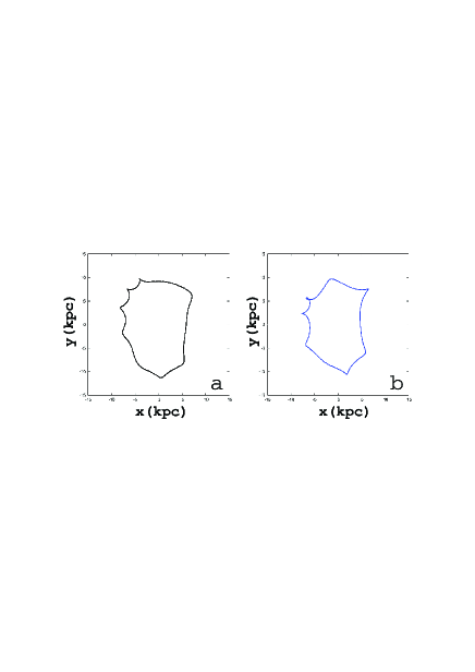
Figure 19: Orbits of the families 8/1 (a) and 7/1 (b) in Model 2.

Figure 20: Histogram that presents the Jacobi constant statistics of the particles in an isolated region that includes the spirals, but not the bar, in the response Model 2.

The reason for which we have the formation of an open spiral and not a ring is that the orbits that participate in the formation of the structure are chaotic. Longer stability intervals along the characteristics of the involved families would trap a large number of quasi-periodic orbits around them leading to the formation of rings on the response models. Even the size of the islands of the stable 8/1 orbits are tiny, so the amount of trapped orbits is small. However, despite the fact that the stable periodic orbit influences a small part of the phase space and the fact that apart from the 8/1 family all other periodic orbits are unstable, we observe a similarity between the morphology of the existing periodic orbits (see Fig. 19) and the chaotic orbits that support the spiral structure (Fig. 21). This dynamical behaviour is similar to the one found by Patsis et al. (1997) for the orbits that support the outer envelope of the bar in the potential of NGC 4314.

Model 2 gave an acceptable solution for the spirals of NGC 1300. However, out of the morphological features of the bar only its size matches the size of the NGC 1300 bar. The combination of the two acceptable solutions, namely Model 1 for the bar and Model 2 for the spirals, in a single model with two pattern speeds is problematic. A careful inspection of the NGC 1300 morphology shows that a bar rotating with a different pattern speed than the spirals will after a certain time visit the spiral region and the combined structure will change drastically in time. A way out of this dilemma is offered by our next model we have chosen to present, i.e Model 3.

4 Model 3

The two models we have presented up to now have a planar geometry. For models in the general class of thick disc models (PI), we have realized in PII, that in the range of $\Omega_{p}$ around 16 km s^-1 kpc^-1 $\!,$ the bar was becoming considerably thinner than the corresponding 2D models with the same pattern speed. In this section we describe the orbital behaviour in a thick disc model (see PI), rotating with $\Omega_{p}$=16 km s^-1 kpc^-1 ​. Around this $\Omega_{p}$ value the $d_{GH}$ index in PII improves in models, where we weight the Jacobi constants we use in our models. However, the thinning of the bar and the enhancement of the density at the ends of the bar that emphasizes its ansae character, is a basic feature of all thick disc models with relatively low patterm speeds. The best similarity with the NGC 1300 image is observed at $\Omega_{p}$=16 km s^-1 kpc^-1 (see Fig. 3 in PII). The $R_{CR}/R_{b}$ ratios we find considering the L₁ and L₂ Lagrangian points are this time 1.5 and 1.7 respectively.

The response of our Model 3 is given in Fig. 22. The feature that appears considerably improved compared with Model 2 is the bar. The length of the bar remains the same, however the ends of the bar appear thinner and elongated at the region which corresponds to the ansae of the NGC 1300 bar (see also the corresponding section in PII). On the other hand less successful is the model in describing the spiral of the galaxy. At the same region, where we obtained the spiral arms in the 2D Model 2, now a ring is formed. The density along this ring is not constant, but the resulting feature does not match the spiral of the galaxy as good as the model with the planar geometry (cf. Figs. 15 and 22). Below we describe the differences in the orbital dynamics between the two models, that are reflected in the morphology of their responses.

The evolution of the (E_J , $x$) characteristics of the main families of periodic orbits for Model 3 is given in Fig. 23. In contrast with Model 2, the x1 characteristic is stable also at the raising part of the curve beyond E_J $\approx-237000$. Simultaneously, already for E_J $\gtrapprox-232000$, there exists a stable 4/1 family, symmetric, with orbits of rhomboidal morphology. The families attributed to higher order resonances (7/1, 8/1) still exist, and even at a larger Jacobi constant interval than in Model 2. This time we find a stable part at the 7/1 characteristic, as well as a small stable part of 8/1. The morphology of the orbits of these families is similar to that of the corresponding families of the planar model (Fig. 19). Finally, we mention the presence of several 3/1 families, also with stable parts, at $-233000\lessapprox$ E_J $\lessapprox-224000$.

Looking first for bar supporting orbits, we have found that they belong to x1, 4/1 and even to 3/1 families. In Fig. 24 we present stable bar supporting periodic orbits with loops, that can be considered as a skeleton of a bar structure. An arrow labeled “a” points to the innermost orbit, which belongs to the x1 family and has E_J = $-250000$. The morphological evolution of x1, also in this model, follows that of the propeller orbits described in Kaufmann & Patsis (2005). Orbit “b”, belongs also to the x1 family, has E_J = $-235000$, i.e. it is at the beginning of the raising part of the x1 characteristic. The third orbit of the sample, named “c”, is from the 4/1 rhomboidal family at E_J = $-230000$ and has asymmetric loops, with the lower loop being larger than the upper one. Finally the outermost periodic orbit, “d”, is an orbit of multiplicity 3, the characteristic of which is the segment, like an extension, at the local maximum of the 4/1 characteristic. This orbit has E_J =$-224000$.

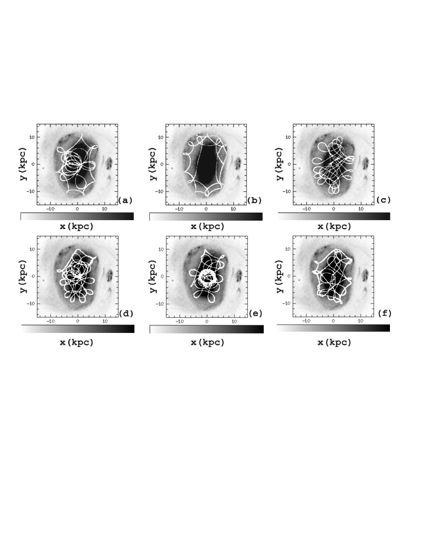
Figure 21: Typical spiral supporting orbits in Model 2 with E_J =$-153500$ in the upper row (panels (a), (b) and (c)) and with E_J =$-155000$ in the lower row (panels (d), (e) and (f)). The spirals are supported by the loops of the orbits at their region. At the background we give the response Model 2.

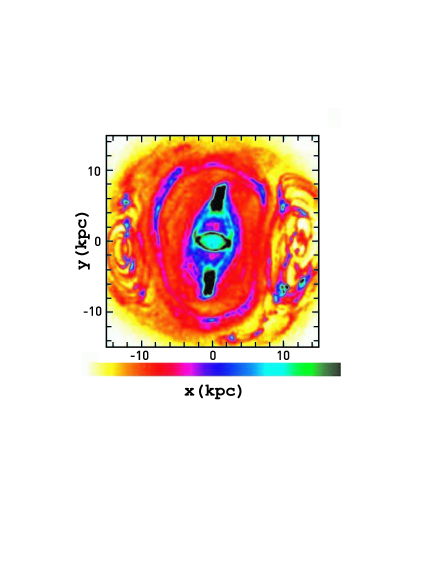
Figure 22: The color-scaled density response of our Model 3, a thick disc model rotating with $\Omega_{p}$=16 km s^-1 kpc^-1 ​.

Model 3 differs from the other models studied up to now, in that there are always stable bar supporting orbits up to the 4/1 resonance region. Besides the stable simple periodic orbits the surfaces of section are characterized by the presence of islands of stable periodic orbits of higher multiplicity and sticky regions around them. We give a typical example in Fig. 25. It is the (x,ẋ) surface of section for E_J =$-228000$. The stable periodic orbit at the center of the island of stability belongs to the 4/1 family. Its shape is indicated in a box at the lower right corner of the figure. Another stable periodic orbit at this Jacobi constant is a periodic orbit of multiplicity three. The three islands of stability, to the left of the 4/1 island, belong to it and its shape is presented in a box at the upper left corner of Fig. 25. Note the darker areas, that appear as bridges between the islands of the triple orbit and the island of stability of the 4/1 orbit. As we can observe from the morphology of these two periodic orbits both of them are bar supporting. Bar supporting are also the sticky and other chaotic orbits that we integrated for time equal to seven pattern rotations. We can say, that the bar of Model 3 is built to a large extent in the classical way, i.e. with regular orbits trapped around stable periodic orbits. This bar has many common features with the NGC 1300 bar.

5 Model 4

We use Model 4 to present another mechanism, that we found to support a spiral structure resembling that of NGC 1300. The mechanism involves orbits around the Lagrangian points L₄ and L₅. The efficiency of this mechanism in supporting spirals was more evident in models with thick discs, especially in the range 20 km s^-1 kpc^-1 $<\Omega_{p}<$23 km s^-1 kpc^-1 ​. Model 4 is a thick disc model (see PI) rotating with $\Omega_{p}=$22 km s^-1 kpc^-1 ​.

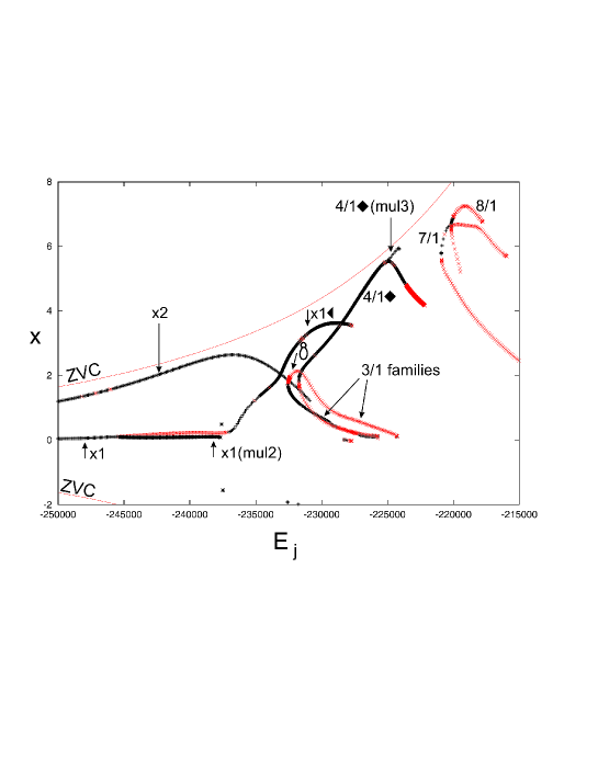
Figure 23: The (E_J , $x$) characteristics of the main families of periodic orbits of Model 3. Black indicates stable orbits, while grey (red in the online version)

unstable.

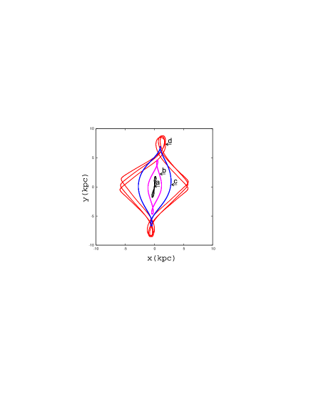
Figure 24: Bar building orbits in Model 3. The two innermost orbits belong to x1, while the two outermost to the 4/1 rhomboidal family.

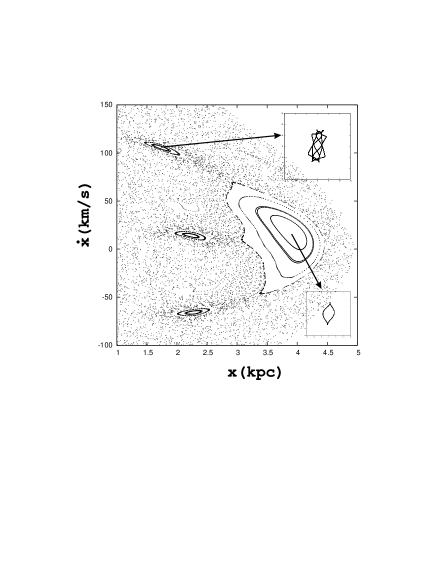
Figure 25: Part of the surface of section of Model 3 for E_J =$-228000$. The big island belongs to a stable orbit of the 4/1 family, while the three islands to a triple periodic orbit. The morphology of the two orbits is given in boxes.

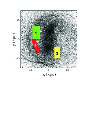
Figure 27: The three regions (“1”, “2” and “3”) at which we examine the Jacobi constants of the particles participating in the spiral structure of Model 4

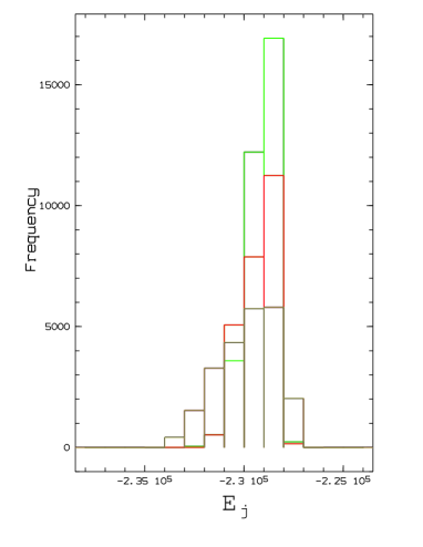
Figure 28: Histogram giving the statistics of the Jacobi constants at the three selected regions of the spirals in Model 4. Green and red correspond to the regions “1” and “2” respectively in Fig. 27, while the particles of region “3” are represented by the yellow-grey bars.

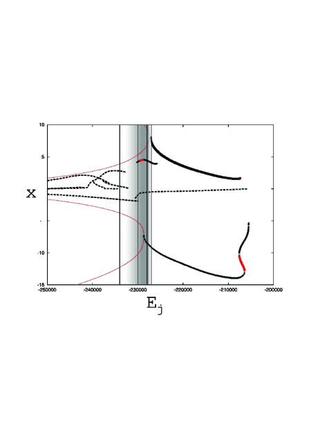
Figure 29: The (E_J ,$x$) diagram for the main families in Model 4. Only the families drawn with heavy lines play a role in the formation of the spirals of the model. The vertical lines indicate the extent of the interval of Jacobi constants we study (see text).

The overall response of the model and the relation of it with the K-band morphology of NGC 1300 is given in Fig. 26. The best reproduced feature of this model with respect to the rest of the models we have examined until now is the beginning of the left spiral, which emerges from the lower end of the bar. There is clearly an increase of the local density of the model along the direction, where the left spiral of the galaxy extends, as we can see in Fig. 26b. We also can observe that the right spiral arm of the model breaks at about the same region as the spiral of the galaxy and also that there is an increase of the local density of the model close the lower end of the bar, at the right side, in general agreement with the fragment of spiral arm we find at the same region at the image of the galaxy. A feature of the effective potential of this model worth pointing out is the characteristic asymmetry of the Lagrangian points L₁ and L₂ with respect to the major axis of the bar. The $R_{CR}/R_{b}$ ratios we find for this model considering the L₁ and L₂ Lagrangian points, are 1.15 and 1.16 respectively. We have taken three sets of particles from three dense regions of the model spirals in order to find their Jacobi constants. This is given in Fig. 27, where these regions are labeled with “1” (upper part of the left arm), “2” (lower part of the right arm) and “3” (spiral segment at the right side, close to the lower end of the bar). The statistics of the Jacobi constants are given in Fig. 28. Green and red correspond to the the boxes labeled with “1” and “2” in Fig. 27 respectively, while the histogram of region “3” is given in yellow-grey. The peak of the Jacobi constants of the particles in all three regions is at $-229000<$ E_J $<-228000$, while we observe, that the Jacobi constants of all particles we consider, have $-234000<$ E_J $<-227000$. So we focus our investigation to spiral supporting orbits at these Jacobi constants. As regards periodic orbits, we give in Fig. 29 with heavy lines the (E_J ,$x$) characteristics of the families that are involved in the enhancement of the spiral arms in Model 4. The left and right vertical lines indicate the extent of the E_J interval that we have to investigate as results from the statistics presented in Fig. 28, i.e. $-234000<$ E_J $<-227000$. The two lines between them show the part of the interval, where we have the two highest bars of the histogram, i.e they are at E_J =$-230000$ and $-228000$ respectively. The darkness of the grey shade reflects the number of particles at the bins of the histogram in Fig. 28. Essentially the interval of the Jacobi constants we study includes parts of the characteristics of three families with stable parts. L₄ and L₅ are stable in this model. We study two characteristic surfaces of section for two close by values of E_J . In Fig. 30 we present them for E_J =$-229000$ in (a) and for E_J =$-228000$ in (b). In (a) we are located still before the local maximum of the ZVC at negative $x$’s, close to L₅. The surface of section is practically chaotic everywhere. However, we discern a darker region at the right side of the left part of the surface of section. In (b) the two regions, the central and the left one, have merged and a family of stable banana like orbits, originated at L₅ appears (invariant curves in the dense region at $x\approx-10$ kpc). It is surrounded by a sticky region, while another dark, sticky, region can be observed at the right part of the central region. We followed the same procedure as in the previous models and we integrated for time equal to 7 pattern rotations a large number of initial conditions on both surfaces of section of Fig. 30.

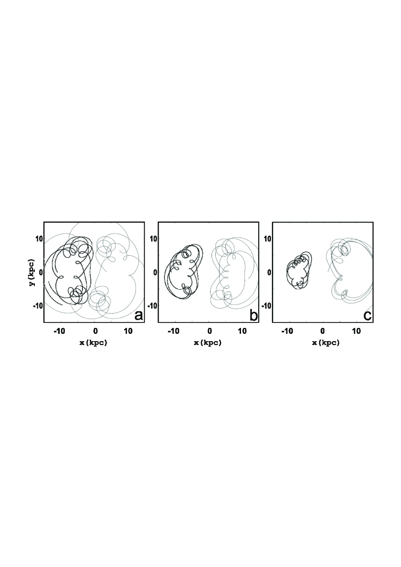
Figure 31: Orbits at the sides of the bar in Model 4, with E_J =$-229000$. With black we give orbits at the left and with grey at the right side of the bar.

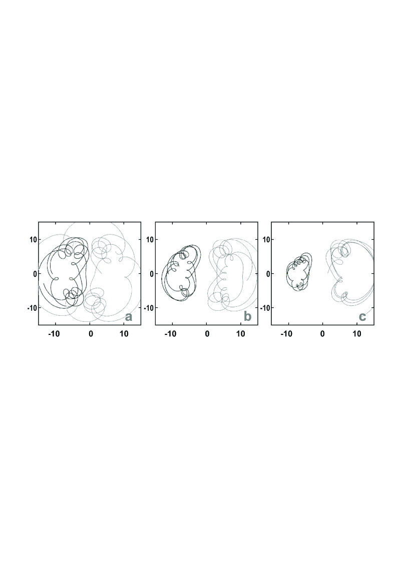
Figure 32: Orbits at the sides of the bar in Model 4, with E_J =$-228000$. Black orbits surround L₅, while grey L₄.

In the subsequent figures we group the orbits of the particles on the spirals as follows: Figure 31 presents characteristic orbits at the sides of the model bar. With grey are the trajectories at the right side. We observe the loops at areas that correspond to the ends of the right side of the bar. Simultaneously these orbits leave rather empty the region between 5$<x<$10 kpc. With black are given orbits at the left side of the bar this time. Most of the loops of these orbits are along the region of the left spiral arm of the model, while at their lower left side they perform in most cases a single loop that brings them closer to the bar. More efficiently acts this mechanism at E_J =$-228000$. For the same reasons we explained in the case of E_J =$-229000$, the orbits at Fig. 32, which have E_J =$-228000$, contribute to the formation of the spiral features. With black we give orbits of various sizes surrounding L₅. The loops of the large size orbits enhance the lower and upper part of the left spiral arm, while the small sized contribute to the formation of the central part. With grey we give orbits surrounding L₄.

Summarizing the response of Model 4 we can say, that density maxima aligned along the location of the spiral arm features of NGC 1300, are provided by the banana-like orbits. It is remarkable also that the characteristic break of the right arm, just after it emerges from the bar, and the presence of the spiral segment close to the lower right end of the bar are also reproduced in an acceptable degree by Model 4 (Fig. 26). However, the drawback of the mechanism is that one cannot get rid of the additional features that are brought in the model from the same orbits that reinforce the spirals. As we can see in Fig. 26b, there is a lot of additional structure that appears together with the spirals to the left of the spiral arm. This structure is formed by the part of the orbits that is far from the bar. It is a quite robust feature and cannot be smoothed out even by increasing the dispersion in the velocities of the initial conditions of response models with $20<\Omega_{p}<24$ km s^-1 kpc^-1 , always in the thick disc approximation.

We finally note that in Model 4 we have the clear evolution of two spiral features that start with an overdense region almost on the major axis of the bar, but away from it. The lower of the two starts in Fig. 26 at about $(x,y)\approx(-2,-14)$ and goes out of the frame at $(-15,-8)$. This feature, as well as its symmetric with respect to the center of the galaxy at the upper part of the model, are related with orbits associated with the outer resonances, beyond corotation (Kaufmann & Contopoulos, 1996). However, it seems that they do not have any correspondence in the near-infrared morphology of NGC 1300.

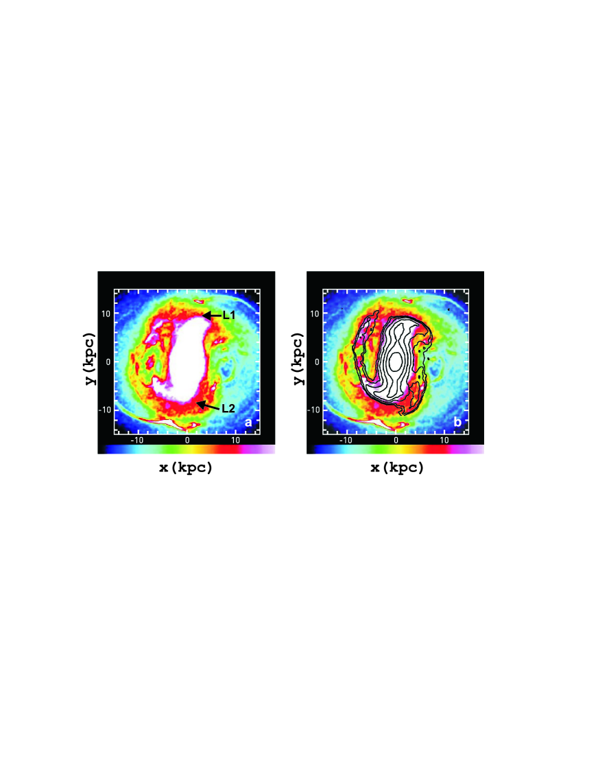
Figure 26: The color-scaled density response of Model 4. It is a thick disc model rotating with $\Omega_{p}=$22 km s^-1 kpc^-1 ​. In (a) the location of L₁ and L₂ are indicated with arrows. In (b) we overplot characteristic isophotes of the K-band image of NGC 1300.

6 Other cases examined

The class of models that is not represented in our analysis is the one that assumed a spherical component representing the major part of the bar (without the ansae) (see PI). This class of models did not improve the resemblance between model and galaxy. However, in PII we have seen that the model of this class especially with $\Omega_{p}=21$ km s^-1 kpc^-1 had a closer resemblance to the galaxy in its very central part. The orbital analysis has shown that the inclusion of an extended spherical component introduces in the system circular, and nearly circular, x1 orbits at the major part of the characteristic of this family. The characteristic remains close to the $x=0$ axis at long E_J intervals. In the particular model the presence of the circular x1 orbits secures a round central region of radius $\approx$ 0.5 kpc. For larger Jacobi constants the orbits of the x1 family become asymmetric with respect to the x-axis. Their morphology becomes elliptical with one focus at the origin of the axes of our system and the other at negative y. This follows the tendency of the central region of the galaxy to become elongated towards negative y. The results of all models presented here do not alter qualitatively even if we chose different projection parameters on the sky for the disc of NGC 1300. We find similar dynamical mechanisms acting also for the projection parameters (PA, IA)=106.6${}^{\circ},42.2^{\circ}$), which are those one finds by fitting an exponential disc to the regions outside the main bar in the K-band image, as in Grosbøl et al. (2004) in agreement with Laurikainen & Salo (2002). A few examples have been presented in Patsis & Kalapotharakos (2008). The dynamical mechanisms are similar, the $\Omega_{p}$ numerical values however, differ.

7 Discussion and Conclusions

Following the framework established in PI, we performed extensive modeling of the stellar component of NGC 1300 in three classes of models reflecting different geometries. As we have seen in PII, we obtained acceptable solutions for the bar or the spirals not only for more than one pattern speed, but for different geometries as well. Anyhow, the main parameter that determines the morphology of our response models is $\Omega_{p}$. The orbital analysis of the present paper, shed light on the various “promising” models and provided feedback, that could be used for the determination of the optimum solution. However, the most interesting result was not the determination of the optimum parameters for a “best” NGC 1300 model, but the dynamical mechanisms themselves, which are leading to the desired morphology. Even models to which our analysis was not pointing to as best matching the NGC 1300 morphology, have a special interest, since their parameters are equally realistic for a barred-spiral system in general as those best applying to the specific galaxy.

Summarizing the four models we have chosen to present, we found that there have been two values of $\Omega_{p}$ for which our models were giving the best matching morphologies to NGC 1300 in the three classes of models we considered, namely $\Omega_{p}$=16 km s^-1 kpc^-1 and 22 km s^-1 kpc^-1 ​. The new dynamical mechanisms that we found deserving special attention and extensive presentation, were the following:

• In a 2D model rotating with $\Omega_{p}$=22 km s^-1 kpc^-1 ​, a strong bar with ansae is supported practically only by chaotic orbits. This bar has similar morphology with the bar of NGC 1300. Decisive role in the support of such a structure by chaotic orbits plays the presence on the effective potential of multiple Lagrangian points roughly along the major axis of the bar. We can understand this by considering an $\Omega(r)$ curve, which is not monotonically decreasing, but has a wavy character. Then it is possible to get the same $\Omega_{p}$ at two (or more) points along the $\Omega(r)$ curve. This is the case of the bar in our Model 1. It is an alternative mechanism for the support of the ansae morphology based only on chaotic orbits. Probably it can be applied to many bars showing this feature.

• In a 2D model rotating with $\Omega_{p}$=16 km s^-1 kpc^-1 ​, our Model 2, the morphology of the spiral arms of NGC 1300 can be reproduced by chaotic orbits at E_J ’s between the 4/1 resonance and corotation. In our case the E_J values of the orbits that support the spirals are well inside corotation. The spirals are supported by the “bouncing” of the chaotic orbits on the “walls” of the effective isopotential drawn with a heavy line in Fig. 16.

• In a thick disc model rotating with $\Omega_{p}$=22 km s^-1 kpc^-1 ​​, we found a mechanism supporting a spiral structure similar to that of NGC 1300 with orbits around the Lagrangian points L₄ and L₅ (our Model 4). These orbits are either regular orbits trapped around stable periodic orbits at the region, or sticky chaotic orbits, or even chaotic trajectories from a pool of a chaotic sea. All of them contribute to the support of the spiral arms. The possibility that a set of banana-like orbits can support a spiral morphology has been indicated by Patsis (2006) and Contopoulos (2009) (see also Contopoulos, 2006).

We do not include in our enumeration of the new mechanisms the formation of a typical ansae bar by regular orbits as in our Model 2.

By “chaotic orbits” we actually mean trajectories, that occur after integrating for a given time initial conditions, which we select out of a common chaotic sea, i.e. essentially we examine fragments of a single chaotic orbit. If at a certain E_J a percentage of these trajectories supports a given structure (a bar or a spiral) it practically means, that the orbit that fills the chaotic sea supports this structure during the same percentage of its, long, integration time. Our result, that surfaces of section without any discernible island of stability provide support to a specific morphological feature, means that the chaotic sea is structured in such a way, that allows this dynamical behaviour. Despite the fact, that there is no obvious structure in a chaotic sea, it is known that the manifolds associated with the unstable periodic orbits existing on the surface of section do structure the chaotic sea (e.g. Contopoulos, 2004). In our models the spirals that we discuss as reproducing the spiral arms of NGC 1300 are inside corotation. However, the general relation between manifolds and resulting spiral structure is expected to be similar to the one described by Tsoutsis et al. (2008), Tsoutsis et al. (2008) and Tsoutsis et al. (2009) for spirals related with the family of unstable periodic orbits originated at the unstable Lagrangian points L₁ and L₂ at corotation. We do not point to a specific family of unstable orbits, the existence of which determines that of the spirals in Model 2 or the ansae type bar in Model 1. It is the collective dynamical behaviour in chaotic seas within a specific E_J range. The dynamical mechanisms that shape a structure are in general different. In Model 2 it is the restriction of the chaotic orbits by a characteristic isocontour of the effective potential and the loops of the orbits as they “bounce” on it. On the other hand in Model 1 it is the trapping of the orbits in the central area and the presence of the double L₁ points that shape the morphology of the bar. The structures that are supported by chaotic orbits are dictated to a large extent by the shape of the isocontours of the effective potential. The fact that star clusters in the spiral arms of NGC 1300 are not well aligned as in other grand-design spiral galaxies (e.g. NGC 2997) (Grosbøl & Dottori, 2008) is in agreement with a chaotic character of the orbits of the stars that build them.

It has been proven quite difficult to point to a best NGC 1300 model. The assumption of different pattern speeds for the bar and the spirals seems less probable, due to the relative locations of the two components. This is not concluded from the apparent connection of the spiral arms and the bar, but mainly from the fact that we do not find two different, separated zones, where bar and spirals rotate without interacting. A bar rotating faster than the spirals will reach the spiral arms at a certain fraction of the spiral period and then there will be an interference between the two components. In such a case the observed morphology would be just a snapshot in a transient morphology of the barred-spiral system. An indication against the transient spiral hypothesis is that the spiral arms exist in K-band and they are even sharp features as we mentioned in the introduction. If we have to deal with a more or less stationary morphology, the regions where bar and spirals rotate should be rather separated. As an example we mention the NGC 3359 model by Patsis et al. (2009), where in a two pattern speeds model the orbits of the spiral component change their topology in such a way as to allow the bar to rotate within a certain radius leaving the spirals outside it (their fig. 20).

From the large number of response models we presented in PII it was evident that it was more difficult to find a response spiral matching the spiral arms of NGC 1300, than to model the bar. The reason is that at a certain range of $\Omega_{p}$ values, in all three general classes of models we studied, the length of the bar is close to the length of the bar of the galaxy. From the two mechanisms that we found supporting the galaxy’s spiral, the one in Model 2 (chaotic orbits between 4/1 and corotation) has more advantages than that of Model 4 (regular and chaotic orbits around L₄ and L₅). Model 2 follows closer the pitch angle of the left arm of NGC 1300, while the spiral fragment at the right of the lower end of the bar is more conspicuous in Model 2 than in Model 4. The chaotic spirals of Model 2 with planar geometry can be combined with the bar of the thick disc Model 3 in a model with a single pattern speed $\Omega_{p}$=16 km s^-1 kpc^-1 ​. On the other hand the left spiral of Model 4 is combined with additional features (Fig. 26, which we cannot ignore in the comparison with the K-band image of the galaxy. There are regions of density maxima to the left of the left arm, that are formed due to the same orbits that give the density maxima along the response density maxima corresponding to the left arm of NGC 1300. These superfluous features could not be eliminated by increasing the velocity dispersion of the initial conditions. By combining Model 1 with Model 4 in a single model rotating with $\Omega_{p}$=22 km s^-1 kpc^-1 ​, we have a 2D bar combined with a spiral in a thick disc beyond the bar. Thus, taking into account the advantages and disadvantages of all models we have found having a good relation with the NGC 1300 morphology we want to model, we conclude that Model 3 for the bar and Model 2 for the stellar spirals, both rotating with $\Omega_{p}$=16 km s^-1 kpc^-1 ​, give the best representation of the corresponding structures of NGC 1300. We underline that the two preferable $\Omega_{p}$ values (16 and 22 km s^-1 kpc^-1 ) are not chosen among equally good models with nearby pattern speeds, but it is a result of the extensive modeling presented in PII, that we have best responses for these two values.

Figure 30: Surfaces of section at E_J =$-229000$ in (a) and for E_J =$-228000$ in (b) in Model 4. At this Jacobi constant we find most particles contributing to the spiral structure.

A comparison of our results with the modeling of NGC 1300 by other authors has been done in PII. We want here to add that our Model 1 gives Lagrangian points (Fig. 2) that are close to the corotation radius of the “fast” model by Lindblad & Kristen (1996), 104$\arcsec$, (L₁, L₂), as well as with the corotation radius of England (1989), $\approx$83 kpc, (L_1S, L₄, L₅). As we explained there is no need for a two pattern speeds assumption for having multiple Lagrangian points in a model.

Below we enumerate our conclusions:

1. We could reproduce structures similar to those of the bar or the spiral of NGC 1300 by more than one model. All models presented in the paper have some nice agreement with the morphology of the galaxy. The comparison of these models with the desired barred-spiral morphology, as well as the comparison among themselves, indicates as best a configuration with a single pattern speed, where the whole barred-spiral structure extends inside corotation. The bar apparently is composed by regular orbits (Model 3), while the stellar spirals are composed by chaotic orbits (Model 2).

2. We find an ansae-type bar morphology that can be constructed completely out of chaotic orbits (Model 1). This requires the presence of multiple unstable Lagrangian points roughly along the major axis of the bar in the effective potential (Fig. 2). This is an alternative way of building ansae-type bars.

3. Chaotic orbits with Jacobi constants between 4/1 and corotation can build a spiral. The dynamical mechanism, described in our Model 2, is based on the loops these orbits perform at their apocentra, as they move in a region defined by the isocontour of the effective potential that separates the regions inside and outside corotation.

4. Another dynamical mechanism that can support a spiral is based on banana-like orbits. These orbits are regular as well as chaotic (Model 4).

5. The recently discussed spirals, that are associated with the stable and unstable manifolds of the unstable Lagrangian points L₁ and L₂, along the major axis of the bar, do not play any important role in our models. We find these spirals in some cases, as the one of Model 1. They emerge from the ends of the bar and fade out after completing an azimuthal distance of about $\pi/2$. However, they are never in agreement with the NGC 1300 spirals.

6. The morphology of the bars and spirals that are supported by chaotic orbits in our models are determined to a large extent by the shape of the isocontours of the effective potential (Figs. 2 and 16).

References

- Athanassoula et al. (2009) Athanassoula E., Romero-Gomez M., Masdemond J.J., 2009, MNRAS 394,67
- Contopoulos (1980) Contopoulos, G., 1980, A&A, 81, 198
- Contopoulos (2004) Contopoulos, G., 2004, “Order and Chaos in Dynamical Astronomy”, 2004, Springer-Verlag, New York
- Contopoulos (2009) Contopoulos, G., 2009, in “Chaos in Astronomy”, Contopoulos G., Patsis P.A. (eds), p. 3, Springer-Verlag Berlin, Heidelberg
- Contopoulos (2006) Contopoulos G. & Patsis P.A. 2006, in “Astrophysical Disks”, Fridman A.M., Marov M.Y., Kovalenko I.G. (eds.), Springer, Dordrecht, The Netherlands, 2006, p.131
- Contopoulos & Patsis (2009) Contopoulos G., Patsis P.A. (eds) 2009, “Chaos in Astronomy”, Springer-Verlag Berlin, Heidelberg
- England (1989) England M., 1989, ApJ 344, 669
- Grosbøl & Dottori (2008) Grosbøl P., Dottori H., 2008, A&A 490,87
- Harsoula & Kalapotharakos (2009) Harsoula M., Kalapotharakos C., 2009, MNRAS 394, 1605
- Hénon (1965) Hénon M., 1965, AnAp, 28, 499
- Kalapotharakos et al. (2010a) Kalapotharakos C., Patsis P. A., Grosbøl P., 2010, MNRAS 403,83 (PI)
- Kalapotharakos et al. (2010b) Kalapotharakos C., Patsis P. A., Grosbøl P., 2010b, submitted (PII)
- Kaufmann & Contopoulos (1996) Kaufmann D.E., Contopoulos G., 1996, A&A, 309, 381
- Kaufmann & Patsis (2005) Kaufmann D.E., Patsis P. A., 2005, ApJ, 624, 693
- Laurikainen & Salo (2002) Laurikainen E., Salo H., 2002, MNRAS, 337, 1118
- Lindblad & Kristen (1996) Lindblad P.A.B., Kristen H. 1996, A&A 313, 733
- Grosbøl et al. (2004) Grosbøl P., Patsis P.A., Pompei E., 2004, A&A, 423, 849
- Patsis (2006) Patsis P.A., 2006, MNRAS 369L, 56
- Patsis et al. (1997) Patsis P. A., Athanassoula E., Quillen A. C., 1997, ApJ, 483, 731
- Patsis & Kalapotharakos (2008) Patsis P. A., Kalapotharakos C., 2010, in ”Tumbling, twisting, and winding galaxies: Pattern speeds along the Hubble sequence”, E. M. Corsini and V. P. Debattista (eds.), Mem.S.A.It, in press (arXiv:1002.1259)
- Patsis et al. (2009) Patsis P. A., Kaufmann, D. E., Gottesman S.T., Boonyasait, V., 2009, MNRAS, 394, 142
- Romero-Gomez et al. (2006) Romero-Gomez M., Masdemont J.J., Athanassoula E., Garcia-Gomez C, 2006, A&A 453, 39
- Voglis et al. (2006) Voglis N., Stavropoulos I., Kalapotharakos C., 2006, MNRAS 372, 901
- Voglis et al. (2006) Voglis N., Tsoutsis P., Efthymiopoulos C. 2006, MNRAS 373, 280
- Tsoutsis et al. (2008) Tsoutsis P., Efthymiopoulos C., Voglis N., 2008, MNRAS 387, 1264
- Tsoutsis et al. (2009) Tsoutsis P., Kalapotharakos C., Efthymiopoulos C., Contopoulos G., 2009, A&A 495, 743