Does Young’s equation hold on the nanoscale? A Monte Carlo test for the binary Lennard-Jones fluid

Abstract

When a phase-separated binary ($A+B$) mixture is exposed to a wall, that preferentially attracts one of the components, interfaces between A-rich and B-rich domains in general meet the wall making a contact angle $\theta$. Young’s equation describes this angle in terms of a balance between the $A-B$ interfacial tension $\gamma_{AB}$ and the surface tensions $\gamma_{wA}$, $\gamma_{wB}$ between, respectively, the $A$- and $B$-rich phases and the wall, $\gamma_{AB}\cos\theta=\gamma_{wA}-\gamma_{wB}$. By Monte Carlo simulations of bridges, formed by one of the components in a binary Lennard-Jones liquid, connecting the two walls of a nanoscopic slit pore, $\theta$ is estimated from the inclination of the interfaces, as a function of the wall-fluid interaction strength. The information on the surface tensions $\gamma_{wA}$, $\gamma_{wB}$ are obtained independently from a new thermodynamic integration method, while $\gamma_{AB}$ is found from the finite-size scaling analysis of the concentration distribution function. We show that Young’s equation describes the contact angles of the actual nanoscale interfaces for this model rather accurately and location of the (first order) wetting transition is estimated.

Introduction and Motivation: Pure fluids and fluid mixtures confined to nanopores are of substantial recent research interest due to various applications, e.g., extraction of oil or gas from porous natural rocks, use as “molecular sieves” to separate fluids, and various applications in nanofluidics such as “lab on a chip”-devices and preparation of materials in nanotechnology, etc. 1 ; 2 ; 3 ; 4 ; 5 ; 6 . At the same time, the interplay between finite-size effects, surface effects due to the pore walls, and interfacial phenomena pose challenging problems to the theoretical understanding on the basis of statistical mechanics 7 ; 8 ; 9 ; 10 . A fundamental concept in this context is the contact angle $\theta$ with which an interface between coexisting (bulk) phases in a phase-separated system meets a wall under conditions of incomplete wetting 7 ; 8 ; 9 ; 10 ; 11 ; 12 ; 13 . In the limit of macroscopically large droplets, for which the droplet radius is many orders of magnitude larger than any interfacial width, one believes that $\theta$ can be expressed in terms of a balance between appropriate interfacial tensions via Young’s equation 14 . For the case of a binary ($A+B$) fluid mixture undergoing phase separation in the bulk into $A$-rich and $B$-rich coexisting phases, this equation reads

$$\gamma_{AB}\cos\theta=\gamma_{wA}-\gamma_{wB},$$ (1)

where $\gamma_{AB}$ is the interfacial excess free energy due to an infinitely extended flat interface between the coexisting bulk phases. In Eq. (1), the excess free energies of the A-rich and B-rich phases due to the wall are denoted by $\gamma_{wA}$ and $\gamma_{wB}$, respectively.

While numerous techniques exist for precise experimental measurements of both the contact angle of macroscopic droplets and the interfacial tension $\gamma_{AB}$, it is challenging to measure $\gamma_{wA}$, $\gamma_{wB}$ independently with sufficient precision. Thus a test of Eq. (1) even for macroscopic droplets is a very difficult task and furthermore, often hampered by substrate inhomogeneities causing contact angle hysteresis 1 ; 11 . For pores in the nanoscale size range, the problem is much harder, since the atomistically diffuse character of the interfaces can no longer be neglected, and of course, in many circumstances interfaces are curved where the understanding of how the interfacial tension $\gamma_{AB}(R)$ varies with the radius of curvature is still incomplete 15 ; 16 ; 17 ; 18 . An additional complication already comes into play for sessile mesoscale droplets attached to walls: then Eq. (1) is modified by a line tension ($\tau$) contribution from the circumference length $2\pi r$ of the sphere-cap shaped droplet right at the wall 19 ; 20 ,

$$\gamma_{AB}\cos\theta=\gamma_{wA}-\gamma_{wB}+\tau/r.$$ (2)

Estimation of the magnitude of the line tension $\tau$ is another problem very controversially discussed in the literature 21 ; 22 ; 23 ; 24 ; 25 . Indeed the proper identification of the line tension effects is subtle 26 . Despite a large experimental and theoretical activity 27 ; 28 ; 29 ; 30 ; 31 ; 32 ; 33 ; 34 ; 35 ; 36 ; 37 for studying capillary condensation, liquid bridges in slit pores, etc., typically the information obtained does not yield both the contact angle and all the excess free energies in Eqs. (1) and (2) with the notable exception of recent simulation studies of the Ising lattice-gas model 36 ; 37 .

The purpose of the present work hence is to provide a first complete test of the validity of Eqs. (1) and (2) in the nano-scale via Monte Carlo simulations of an off-lattice model of a fluid binary mixture. We shall study the structure of liquid bridges of A-rich phases in a B-rich background for various choices of the interactions between the particles and the walls of a nanoscopic slit pore and extract effective contact angles $\theta_{\rm eff}$ to describe the inclined interfaces that occur. In addition, we compute $\gamma_{AB}$ for bulk interfaces and develop a new method to compute $\gamma_{wA}$, $\gamma_{wB}$ for pure semi-infinite phases exposed to corresponding walls. Extending the approach of Winter et al. 36 ; 37 , we are also able to derive the line tension $\tau$ as function of the contact angle $\theta$.

Model and Simulation Technique: Let us consider a binary ($A+B$) fluid consisting of $N$ point particles, labelled by index $i$ at positions $\vec{r}_{i}$, in a box of linear dimensions $L\times L\times D$, with periodic boundary conditions in $x$- and $y$- directions and having impenetrable walls of area $L\times L$ each at $z=0$ and $z=D$. The particles interact via pairwise potentials $u(r_{ij}=|\vec{r_{i}}-\vec{r}_{j}|)$, constructed from the full Lennard-Jones (LJ) potential $\phi_{LJ}(r_{ij})=4\varepsilon_{\alpha\beta}[(\sigma_{\alpha\beta}/r_{ij})^{12}-(\sigma_{\alpha\beta}/r_{ij})^{6}]$, $\alpha,\beta\in A,B$, as 38 ; 39

$$u(r_{ij}\leq r_{c})=\phi_{LJ}(r_{ij})-\phi_{LJ}(r_{c})-(r_{ij}-r_{c})\frac{d\phi_{LJ}}{dr_{ij}}\mid_{r_{ij}=r_{c}},$$ (3)

while $u(r_{ij}\geq r_{c})=0$. This ensures that both the potential and the force are continuous at the cut-off distance $r_{ij}=r_{c}$. The potential parameters are chosen such that the mixture is symmetric: $\sigma_{AA}=\sigma_{BB}=\sigma_{AB}=\sigma$, $\varepsilon_{AA}=\varepsilon_{BB}=2\varepsilon_{AB}=\varepsilon$ and $r_{c}$ was set at $2.5\sigma$. Working at a reduced density $\rho^{*}=1$, where $\rho^{*}=\rho\sigma^{3}=N\sigma^{3}/V$, neither crystallization nor the vapor-liquid transition is a problem, while unmixing occurs for 38 ; 39 $T<T_{c}=1.4230\pm 0.005$ (unit of $T$ is chosen such that $\varepsilon/k_{B}\equiv 1$). Working at $T=1.0$, the bulk A-rich (B-rich) phases are almost pure, $x_{A}^{\rm coex}=(N_{A}/N)_{\rm coex}\approx 0.97$ ($x_{B}^{\rm coex}=0.03$) 18 .

We choose “antisymmetric” interactions of the walls with the fluid particles such that also in the thin film geometry phase coexistence between A-rich and B-rich phases occurs at chemical potential difference $\Delta\mu=0$ between A- and B-particles, as in the bulk 38 ; 39 . Specifically, for the A particles we take a wall potential

$$u_{A}(z)=\frac{2\pi\rho^{*}}{3}\times\quad\quad\quad\quad\quad\quad\quad\quad\quad\quad\quad\quad\quad\quad\quad$$

$$\Big{\{}\varepsilon_{r}\Big{[}\Big{(}\frac{\sigma}{z+\delta}\Big{)}^{9}+\Big{(}\frac{\sigma}{D+\delta-z}\Big{)}^{9}\Big{]}-\varepsilon_{a}\Big{(}\frac{\sigma}{z+\delta}\Big{)}^{3}\Big{\}},$$ (4)

and for the B-particles

$$u_{B}(z)=\frac{2\pi\rho^{*}}{3}\times\quad\quad\quad\quad\quad\quad\quad\quad\quad\quad\quad\quad\quad\quad\quad$$

$$\Big{\{}\varepsilon_{r}\Big{[}\Big{(}\frac{\sigma}{z+\delta}\Big{)}^{9}+\Big{(}\frac{\sigma}{D+\delta-z}\Big{)}^{9}\Big{]}-\varepsilon_{a}\Big{(}\frac{\sigma}{D+\delta-z}\Big{)}^{3}\Big{\}},$$ (5)

where $0\leq z\leq D$ is the coordinate perpendicular to the walls, and the offset $\delta=\sigma/2$. Both the walls exert the same repulsive potential (of strength $\varepsilon_{r}=\varepsilon/2)$ on both kinds of particles. This potential can be thought of as resulting from integration over LJ repulsions from atoms residing in a semi-infinite wall. An attractive interaction (of variable strength $\varepsilon_{a}$) acts only on the A-particles from the wall at $z=0$, while the same acts only on the B particles from the wall at $z=D$.

For direct measurement of $\theta$ from the inclination of $A-B$ interface, Monte Carlo (MC) simulations are carried out in the canonical ensemble where in addition to the standard particle displacement moves, exchange between randomly chosen particle pairs was also tried. For the displacements, a trial shift of a cartesian coordinate of a randomly selected particle in the range $[-\sigma/20$, $+\sigma/20]$ around its old position is chosen and the standard Metropolis criterion applied. On the other hand, thermodynamic integration (see below) was performed by using the raw data obtained from MC simulation in the semi-grand-canonical (SGMC) ensemble. In the latter, after every 10 displacement steps per particle $N/10$ particles are randomly chosen in succession and an attempted identity switch ($A\rightarrow B\rightarrow A$) is made (for more technical details, see 38 ; 39 ). In addition, successive umbrella sampling was performed using SGMC to obtain interfacial free energies of the co-existing phases.

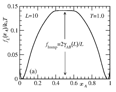
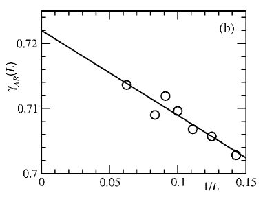
Figure 1: (a) Effective free energy density $f_{L}(x_{A},T)$ of the symmetric LJ mixture at $T=1.0$ for a box of linear dimension $L=10$ (in units of $\sigma$) plotted vs. $x_{A}$. The estimation of the size-dependent interfacial tension $\gamma_{AB}(L)$ is indicated. (b) Extrapolation of $\gamma_{AB}(L)$ as function of $1/L$.

As a first step, we estimate $\gamma_{AB}$ from the finite-size extrapolation of the distribution $P_{L}(x_{A})$ ($x_{A}=N_{A}/N$, the mole fraction of A-particles) using a $L\times L\times L$ geometry, with periodic boundary conditions in all $x$-, $y$- and $z$- directions. Applying successive umbrella sampling 40 , the effective excess free energy density $f_{L}(x_{A},T)$ is found from $f_{L}(x_{A},T)=-(1/V)\ln[P_{\Delta\mu NVT}(x_{A})/P_{\Delta\mu NVT}(x_{A}^{\rm coex})]$. As is well-known 18 ; 37 ; 41 , the flat maximum, $f_{\rm hump}$, in $f_{L}(x_{A},T)$, near $x_{A}=0.5$ in Fig. 1, is due to the formation of two planar $L\times L$ interfaces in the simulation box, separating a slab of A-rich phase from the B-rich phase (or vice versa). Thus this barrier is given by $2\gamma_{AB}(L)/L$ and the extrapolation of such data towards $L\rightarrow\infty$ yields $\gamma_{AB}=0.722\pm 0.002$, as demonstrated in Fig. 1(b).

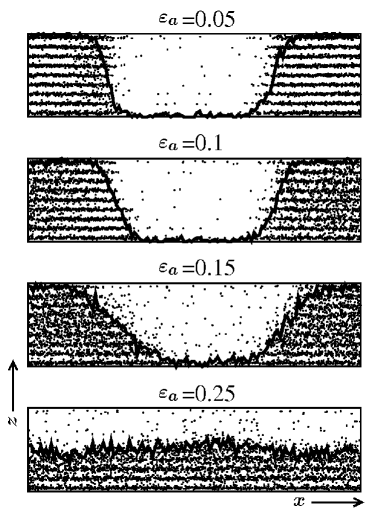
Figure 2: Snapshot pictures of the configurations of the A- particles (dots) in a $L\times L\times D$ system with $L=32$, $D=8$, projected onto the $xz$-plane, for the case of interfaces running along the $y$-direction. B-particles are not shown. Four choices of attractive wall-particle interaction strength $\varepsilon_{a}$ are included, as indicated. The instantaneous interface position (averaged over the $y$ coordinate) is highlighted by thick lines.

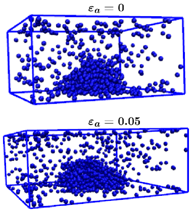
Figure 3: Three-dimensional snapshots of $A-particle$ droplet configurations for the cases $x_{A}=0.12$, $\varepsilon_{a}=0$ ($D=12$, $L=24$; upper part) and $x_{a}=0.12$, $\varepsilon_{a}=0.05$ ($D=12$, $L=30$; lower part).

Interfaces in nano-confinement: Using the model in a $L\times L\times D$ geometry, applying the wall potentials (Does Young’s equation hold on the nanoscale? A Monte Carlo test for the binary Lennard-Jones fluid) and (Does Young’s equation hold on the nanoscale? A Monte Carlo test for the binary Lennard-Jones fluid) and starting with initial configurations prepared such that two $A-B$ interfaces meet the walls vertically, we stabilize two-phase configurations of the system via MC simulation in canonical ensemble for varying strengths of attractive wall potential $\varepsilon_{a}$. For $x_{A}=0.5$ and $\varepsilon_{a}\leq 0.2$ we find slab-like configurations of the B-rich phase as seen in Fig. 2, where the interfaces are represented by thick lines. These interfaces are perpendicular to the $xy$-plane only for $\varepsilon_{a}=0$ when the contact angle $\theta=\pi/2$ by symmetry of our model. For $\varepsilon_{a}>0$ they are inclined relative to the $xy$-plane. We extract an effective contact angle $\theta_{\rm eff}$ from the average slope of these interfaces, measured from the central part of the film, excluding regions of width $2\sigma$ at both walls. For $\varepsilon_{a}=0.25$, wetting has already occurred ($\theta_{\rm eff}=0$) and so, instead of a slab with two interfaces, we now find a single interface, separating the $A$-rich domain near the bottom wall that prefers $A$ from $B$-rich domains near the top wall preferring $B$. One consequence of nano-confinement that one can see in all cases is a pronounced layering of the total density parallel to the confining walls and extending throughout the thin film. If one chooses suitable off-critical concentrations, e.g., $x_{A}=0.12$, one can observe wall-attached droplets shown in Fig. 3, similar to the Ising case 36 ; 37 . The analysis of such states when obtained via umbrella sampling method, thus containing the information of $f_{L}$, allows the estimation of the line tension, when the appropriate contact angle is independently known.

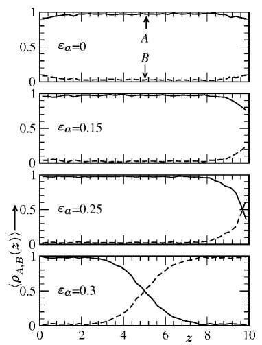
Figure 4: Density profiles $\langle\rho_{A}(z)\rangle$, $\langle\rho_{B}(z)\rangle$, obtained from the semi-grand-canonical MC simulation in a $L\times L\times D$ geometry averaging over $x$ and $y$ coordinates, plotted vs. $z$ for a film of thickness $D=10$. Three top panels ($\varepsilon_{a}=0$, $0.15$ and $0.25$) correspond to the A-rich phases. The panel at the bottom with $\varepsilon_{a}=0.3$ shows the profiles for a state where unbinding of the interface from the wall at $z=D$ has occurred, with the delocalized interface now being at $z=D/2$.

Thermodynamic Integration and Bulk Contact Angle: We consider a film of large but finite thickness in the semi-grand-canonical ensemble with $\Delta\mu=0$ and vary $\varepsilon_{a}$ being in the regime of incomplete wetting, where the system is either in the pure A-rich phase or in the pure B-rich phase, prepared via SGMC simulation. From the density profiles of such systems, as shown in Fig. 4, where the three upper panels correspond to $A$-rich phases (note that in this case only a slight enhancement of $B$ particles could be seen at the wall preferring the latter), one can extract information on $\gamma_{wA}-\gamma_{wB}$ by a thermodynamic integration method. To derive this, we first express the total free energy $F$ of the film via the partition function as a configurational integral

$$F=-k_{B}T\ln Z$$

$$~{}~{}=-k_{B}T\ln\int\limits d\vec{X}\exp\Big{\{}-\beta\mathcal{H}_{b}(\vec{X})-\beta\mathcal{H}^{r}_{w}(\vec{X})$$

$$+\beta\varepsilon_{a}L^{2}(2\pi\rho^{*}/3)\times$$

$$\Big{[}\int\limits_{0}^{D}\langle\rho_{A}(z)\rangle\Big{(}\frac{\sigma}{z+\delta}\Big{)}^{3}dz+$$

$$\int\limits_{0}^{D}\langle\rho_{B}(z)\rangle\Big{(}\frac{\sigma}{D+\delta-z}\Big{)}^{3}dz\Big{]}\Big{\}}.$$ (6)

Here $\beta=1/k_{B}T$ and $\vec{X}$ includes all configurational degrees of freedom of the system. For the sake of brevity, neither the bulk energy $\mathcal{H}_{b}(\vec{X})$ nor the energy $\mathcal{H}^{r}_{w}(\vec{X})$ due to the repulsive part of the wall potential has been explicitly written down. The density profiles $\langle\rho_{A,B}(z)\rangle$ are averaged over $x$ and $y$ coordinates. We now take a derivative with respect to $\varepsilon_{a}$, which singles out the derivatives of the wall free energies $f_{s}$ at $z=0$ and $z=D$, respectively ($f_{s}$ is normalized per unit area)

$$\Big{(}\frac{\partial f_{s}^{(z=0)}}{\partial\varepsilon_{a}}\Big{)}_{T}=\Big{(}2\pi\rho^{*}/3\Big{)}\int\limits_{0}^{D}dz\Big{(}\frac{\sigma}{z+\delta}\Big{)}^{3}\langle\rho_{A}(z)\rangle,$$ (7)

$$\Big{(}\frac{\partial f_{s}^{(z=D)}}{\partial\varepsilon_{a}}\Big{)}_{T} = (2\pi\rho^{*}/3)\times$$ (8)

$$\int\limits_{0}^{D}dz\Big{(}\frac{\sigma}{D+\delta-z}\Big{)}^{3}\langle\rho_{B}(z)\rangle.$$

These equations are readily integrated to yield

$$f_{s}^{(z=0)}(\varepsilon_{a})=f_{s}^{(z=0)}(0)+(2\pi\rho^{*}/3)\times$$

$$\int\limits_{0}^{\varepsilon_{a}}d\varepsilon^{\prime}_{a}\int\limits_{0}^{D}dz\Big{(}\frac{\sigma}{z+\delta}\Big{)}^{3}<\rho_{A}(\varepsilon_{a}^{\prime},z)>,$$ (9)

$$f_{s}^{(z=D)}(\varepsilon_{a})=f_{s}^{(z=D)}(0)+(2\pi\rho^{*}/3)\times$$

$$\int\limits_{0}^{\varepsilon_{a}}d\varepsilon^{\prime}_{a}\int\limits_{0}^{D}dz\Big{(}\frac{\sigma}{D+\delta-z}\Big{)}^{3}<\rho_{B}(\varepsilon^{\prime}_{a},z)>.$$ (10)

Noting that surface free energies of bulk B-rich phases are related to those of the A-rich phases simply by symmetry:

$$f_{s}^{(z=0)}(\varepsilon_{a})\mid_{{B-{\rm rich\,phase}}}=f_{s}^{(z=D)}(\varepsilon_{a})\mid_{{A-{\rm rich\,phase}}},$$ (11)

we immediately obtain the desired difference

$$\gamma_{wA}-\gamma_{wB}\equiv f_{s}^{(z=0)}(\varepsilon_{a})\mid_{A-{\rm rich\,phase}}-$$

$$f_{s}^{(z=0)}(\varepsilon_{a})\mid_{B-{\rm rich\,phase}}$$

$$=(2\pi\rho^{*}/3)\int\limits_{0}^{\varepsilon_{a}}d\varepsilon^{\prime}_{a}\int\limits_{0}^{D}dz\times$$

$$\Big{[}\langle\rho_{A}(\varepsilon^{\prime}_{a},z)\rangle_{{}_{A-{\rm rich}}}\Big{(}\frac{\sigma}{z+\delta}\Big{)}^{3}-$$

$$\langle\rho_{B}(\varepsilon^{\prime}_{a},z)\rangle_{{}_{A-{\rm rich}}}\Big{(}\frac{\sigma}{D+\delta-z}\Big{)}^{3}\Big{]}.$$

In Eq. (Does Young’s equation hold on the nanoscale? A Monte Carlo test for the binary Lennard-Jones fluid) both the profiles $\langle\rho_{A}(\varepsilon^{\prime}_{a},z)\rangle$ and $\langle\rho_{B}(\varepsilon^{\prime}_{a},z)\rangle$ are sampled, without loss of generality, in the A-rich phase, as shown in Fig. 4.

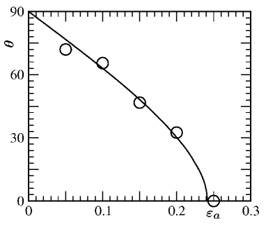
Figure 5: The full curve is a plot of contact angle $\theta$ vs. $\varepsilon_{a}$, as obtained from Young’s equation with the information about $\gamma_{wA}-\gamma_{wB}$ being provided from thermodynamic integration, Eq. (Does Young’s equation hold on the nanoscale? A Monte Carlo test for the binary Lennard-Jones fluid). Circles show corresponding observations from Fig. 2.

Given the knowledge of both the difference $\gamma_{wA}-\gamma_{wB}$ (as function of $\varepsilon_{a}$) and of $\gamma_{AB}$, we can predict the dependence of the contact angle $\theta$ on $\varepsilon_{a}$, as shown in Fig. 5. Following this we obtain the wetting transition ($\theta=0$) at $\varepsilon_{a}=0.240\pm 0.005$. Note also that in our model, for $\varepsilon_{a}=0$ we must have $\theta=\pi/2$ due to the full symmetry between $A$ and $B$ that is present then. Interestingly, the contact angles predicted from Young’s equation, which refer to quasi-macroscopic droplets, agree almost perfectly with the contact angles, represented by circles in Fig. 5, observed in a nanoscopically thin film that is only $8$ Lennard-Jones diameters thick (Fig. 2). Thus Young’s equation still is useful at the nanoscale!

Estimation of the line tension: It would be wrong to conclude from this success of Young’s equation that the line tension does not play any role in our model. In fact for the case $\varepsilon_{a}=0$ it is relatively easy to estimate it from the flat free energy maximum, $f_{\rm hump}$ (cf. Fig. 1(a)), for systems in $L\times L\times D$ thin film geometry by varying $D$. Then one expects that $f_{\rm hump}$ has a value $2\gamma_{AB}/L+4\tau/(LD)$; hence a plot of $Lf_{\rm hump}/(2k_{B}T)$ vs. $2/D$, as presented in Fig. 6, should yield a straight line, where the $y$-intercept is the already known interfacial tension $\gamma_{AB}$, while the slope yields an estimate of $\tau$. In this way we find $\tau\approx-0.52$ for $\varepsilon_{a}=0$. Recall that by symmetry, $\theta=\pi/2$ for $\varepsilon_{a}=0$, irrespective of the presence of the line tension. Unfortunately, when $\varepsilon_{a}>0$ and the interfaces are inclined (Fig. 2), large statistical fluctuations prevent us from using this method. However, following Winter et al. 36 ; 37 we have analyzed the excess free energy of sphere-cap shaped droplets. As will be described elsewhere in detail 42 , the absolute magnitude of $\tau$, obtained from this analysis, decreases rapidly with decreasing contact angle.

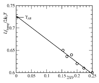
Figure 6: Effective interface tension [estimated via $Lf_{\rm hump}/(2k_{B}T)$] plotted vs. $2/D$, for systems of linear dimensions $L\times L\times D$, with $L=30$ and using several choices of $D$, for the case $\varepsilon_{a}=0$. Arrow shows the estimate of $\gamma_{AB}$ from Fig. 1(b). The straight line is a fit to the form $\gamma_{AB}+2\tau/D$, where both $\gamma_{AB}$ and $\tau$ have been used as adjustable parameters. Fitting gives $\tau=-0.52$ and $\gamma_{AB}=0.725$ [note the agreement with the estimate from Fig. 1(b)].

Summary: In this letter, we have described a study of the contact angle of nanoscale fluid bridges, for a model of a symmetric binary Lennard-Jones mixture, for the full range from neutral walls up to the wetting transition. Supplying the interfacial tensions entering Young’s equation, we observe that the quantitative agreement of the contact angles thus obtained with the direct observation from inclined nanoscopic interfaces in a $50:50$ composition is remarkable. While $\gamma_{AB}$ and the line tension $\tau$ are extracted from suitable system size dependences, $\gamma_{wA}-\gamma_{wB}$ is estimated via a new thermodynamic integration method. Clearly, the symmetric Lennard-Jones mixture is a simple model system, but we expect that our methods can be generalized to more complex models of real fluids. In this way, practically relevant information to guide the development of nanofluidic devices will come in reach.

Acknowledgement: One of us (S.K.D.) is grateful to the Deutsche Forschungsgemeinschaft (DFG) for partial support under grant N^o TR6/A5, and thanks the Institut für Physik, Mainz, for hospitality during his research visits. We are grateful to J. Horbach, M. Oettel and P. Virnau for stimulating discussions.

References

- (1) GELB L.D., GUBBINS K.E., RADHAKRISHNAN R., SLIWINSKA-BARTKOVIAK M., Rep. Progr. Phys. 62 (1999) 1573.
- (2) ROUQUEROL F., ROUQUEROL J., SING K.S.W, Adsorption by Powders and Porous Solids: Principles, Methodology, and Applications (Academic Press, San Diego) 1999.
- (3) THORSEN T., MAERKL S.J., QUAKE S.R, Science 298 (2002) 580.
- (4) MELLER A., J. Phys.: Condens. Matter 15 (2003) R581.
- (5) WOLF E.L., Nanophysics and Nanotechnology (Wiley-VCH, Weinheim) 2004.
- (6) SQUIRES T.M, QUAKE S.R, Rev. Mod. Phys. 77 (2005) 977.
- (7) ROWLINSON J.S., WIDOM. B, Molecular Theory of Capillarity (Oxford Univ. Press, Oxford) 1982.
- (8) CROXTON C.A. (ed.), Fluid Interfacial Phenomena (Wiley, New York) 1985.
- (9) CHARVOLIN J., JOANNY J.F., ZINN-JUSTIN J. (Eds), Liquids at Interfaces (North-Holland, Amsterdam) 1990.
- (10) HENDERSON D. (Ed.), Fundamentals of Inhomogeneous Fluids (Dekker, New York) 1992.
- (11) DE GENNES P.G, Rev. Mod. Phys. 57 (1985) 827.
- (12) DIETRICH S., in Phase Transitions and Critical Phenomena, Vol XII, p.1, DOMB C., LEBOWITZ J.L. (Eds.), (Academic Press, New York) 1988.
- (13) BONN D., ROSS D., Rep. Progr. Phys. 64 (2001) 1085.
- (14) YOUNG T., Phil. Trans. R. Soc. London 95 (1805) 65.
- (15) TOLMAN R.C., J. Chem. Phys. 17 (1949) 333.
- (16) GRANASY L., J. Chem. Phys. 109 (1998) 9660.
- (17) VAN GIESSEN A.E., BLOKHUIS E.M., J. Chem. Phys. 131 (2009) 164705.
- (18) BLOCK B.J., DAS S.K., OETTEL M., VIRNAU P., BINDER K., preprint.
- (19) GRETZ R.D., J. Chem. Phys. 45 (1966) 3160.
- (20) NAVASCUES G., TARAZONA P., J. Chem. Phys. 75 (1981) 2441.
- (21) INDEKEU J.O., Int. J. Mod. Phys. B 8 (1994) 309.
- (22) DRELICH J., Colloids and Surfaces A 116 (1996) 43.
- (23) AMIRFAZLI A., HÄNIG S., MÜLLER A., NEUMANN A.W., Langmuir 16 (2000) 2024.
- (24) MUGELE F., BECKER T., NIKOPOULOS R., KOHONEN M., HERMINGHAUS S., J. Adhesion Sci. Technol. 16 (2002) 951.
- (25) LEFEVRE B., SAUGEY A., BARRAT J.L., BOCQUET L., CHARLAIX E., GOBIN P.F., VIGIER G., J. Chem. Phys. 120 (2004) 4927.
- (26) SCHIMMELE L., NAPIORKOWSKI M., DIETRICH S., J. Chem. Phys. 127 (2007) 164715.
- (27) EVANS R., MARINI BETTOLO MARCONI U., TARAZONA P., J. Chem. Phys. 84 (1986) 2376.
- (28) EVANS R., J. Phys.: Condens Matter 46 (1990) 9899.
- (29) CRASSOUS J., CHARLAIX E., GAYWALLET H., LOUBET J.-L., Langmuir 9 (1993) 1995.
- (30) CRASSOUS J., CHARLAIX E., LOUBET J.-L., Europhys. Lett. 28 (1994) 37.
- (31) VALENCIA A., BRINKMANN M., LIPOWSKY R., Langmuir 17 (2001) 3390.
- (32) YANEVA J., MILCHEV A., BINDER K., J. Chem. Phys. 121 (2004) 12632.
- (33) SCHOEN M., KLAPP S.H.L., Reviews of Computational Chemistry, Vol 24 (Wiley, New York) 2007.
- (34) BROVCHENKO I., OLEINIKOVA A., Interfacial and Confined Water (Elsevier, Amsterdam) 2008.
- (35) BINDER K., HORBACH J., VINK R.L.C., DE VIRGILIIS A., Soft Matter 4 (2008) 1555.
- (36) WINTER D., VIRNAU P., BINDER K., Phys. Rev. Lett. 103 (2009) 225703.
- (37) WINTER D., VIRNAU P., BINDER K., J. Phys.: Condens. Matter 21 (2009) 464118.
- (38) DAS S.K., HORBACH J., BINDER K., FISHER M.E., SENGERS J.V., J. Chem. Phys. 125 (2006) 024506.
- (39) DAS S.K., FISHER M.E., SENGERS J.V., HORBACH J., BINDER K., Phys. Rev. Lett. 97 (2006) 025702.
- (40) VIRNAU P., MÜLLER M., J. Chem. Phys. 120 (2004) 10925.
- (41) BINDER K., Phys. Rev. A 25 (1982) 1699.
- (42) DAS S.K., BINDER K., to be published.