Theory of magnon-driven spin Seebeck effect

Abstract

The spin Seebeck effect is a spin-motive force generated by a temperature gradient in a ferromagnet that can be detected via normal metal contacts through the inverse spin Hall effect [K. Uchida et al., Nature 455, 778-781 (2008)]. We explain this effect by spin pumping at the contact that is proportional to the spin-mixing conductance of the interface, the inverse of a temperature-dependent magnetic coherence volume, and the difference between the magnon temperature in the ferromagnet and the electron temperature in the normal metal [D. J. Sanders and D. Walton, Phys. Rev. B 15, 1489 (1977)].

I Introduction

The emerging field called spin caloritronics addresses charge and heat flow in spin-polarized materials, structures, and devices. Most thermoelectric phenomena can depend on spin, as discussed by many authors in Ref. special_issue, . A recent and not yet fully explained experiment Uchida et al. (2008) is the spin anologue of the Seebeck effect — the spin Seebeck effect, in which a temperature gradient over a ferromagnet gives rise to an inverse spin Hall voltage signal in an attached Pt electrode.

The Seebeck effect refers to the electrical current/voltage that is induced when a temperature bias is applied across a conductor. By connecting two conductors with different Seebeck coefficients electrically at one end at a certain temperature, a voltage can be be measured between the other two ends when kept at a different temperature. The spin counterpart of such a thermocouple is the spin current/accumulation that is induced by a temperature difference applied across a ferromagnet, interpreting the two spin channels as the two “conductors”. In Uchida et al.’s experiment, Uchida et al. (2008) a temperature bias is applied over a strip of a ferromagnetic film. A thermally induced spin signal is measured by the voltage induced by the inverse spin Hall effect (ISHE) Valenzuela and Tinkham (2006); Kimura et al. (2007) in Pt contacts on top of the film in transverse direction (see Fig. 1). This Hall voltage is found to be approximately a linear function (possibly a hyperbolic function with long decay length) of the position in longitudinal direction over a length of several millimeters. This result has been puzzling, since spin-dependent length scales are usually much smaller. The original explanation for this experiment has been based on the thermally induced spin accumulation in terms of the spin thermocouple analogue mentioned above. However, the spin flip scattering shot-circuits the spin channels, and at which spin channels are shot-circuited, the signal should vanish on the scale of the spin-flip diffusion length. hatami_2009

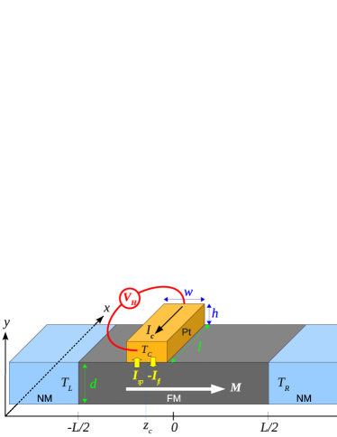
Figure 1: (Color online) A ferromagnet (F) with thickness $d$ and length $L$ and magnetization $\mathbf{M}$ pointing in $\hat{\mathbf{z}}$-direction connects two normal metal (N) contacts at temperature $T_{L/R}$ at the left and right ends. A Pt strip of dimension $l{\times}w{\times}h$ on top of F converts an injected spin current (${\bf I}_{s}={\bf I}_{sp}+{\bf I}_{fl}$) into an electrical current $I_{c}$ or Hall voltage $V_{H}$ by the inverse spin Hall effect.

In this paper, we propose an alternative mechanism in terms of spin pumping caused by the difference between the magnon temperature in the ferromagnetic film and the electron temperature (assumed equal to the phonon temperature) in the Pt contact. Such a temperature difference can be generated by a temperature bias applied over the ferromagnetic film. Sanders and Walton (1977)

This paper is organized as follows: Section II describes how a DC spin current is pumped through a ferromagnet(F)—normal metal(N) interface by a difference between the magnon temperature in F and electron temperature in N. In section III we calculate the magnon temperature profile in F under a temperature bias. In Section IV we compute the thermally driven spin current as a function of the position of the normal metal contact.

II Thermally driven spin pumping current across F—N interface

In this Section we derive expressions for the spin current flowing through an F—N interface with a temperature difference as shown in Fig. 2, starting with the macrospin approximation in Subsection II.A and considering finite magnon dispersion in Subsection II.B.

Since the relaxation times in the spin, phonon, and electron subsystems are much shorter than the spin-lattice relaxation time, Kittel and Abrahams (1953); Demokritov et al. (2006) the reservoirs become thermalized internally before they equilibrate with each other. Therefore, we may assume that the phonon (p), conduction electron (e), and magnon (m) subsystems can be described by their local temperatures: $T_{F}^{p,e,m}$ in F, and $T_{N}^{p,e}$ in N. Beaurepaire et al. (1996) We furthermore assume that the electron-phonon interaction is strong enough such that locally $T_{F}^{p}=T_{F}^{e}{\equiv}T_{F}$ and $T_{N}^{p}=T_{N}^{e}{\equiv}T_{N}$. However, the magnon temperature may deviate: $T_{F}^{m}{\neq}T_{F}$. This is illustrated below by the extreme case of the macrospin model, in which there is only one constant magnetic temperature, whereas the electron and phonon temperatures linearly interpolate between the reservoir temperatures $T_{L}$ and $T_{R}$. The difference between magnon and electron/phonon temperature therefore changes sign in the center of the sample. When considering ferromagnetic insulators, the conduction electron subsystem in F becomes irrelevant.

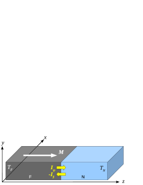
Figure 2: (Color online) F—N interface with 1) spin pumping current ${\bf I}_{sp}$ driven by the thermal activation of the magnetization in F at temperature $T_{F}$, and 2) fluctuating spin current ${\bf I}_{fl}$ driven by the thermal activation of the electron spins in N at temperature $T_{N}$.

II.1 F—N contact

First, let us consider a structure such as shown in Fig. 2, in which the magnetization is a single domain and can be regarded as a macrospin ${\bf M}=M_{s}V\mathbf{m}$, where $\mathbf{m}$ is the unit vector parallel to the magnetization. We will derive in Subsection II.B the criteria for the macrospin regime. We assume uniaxial anisotropy along $\hat{\mathbf{z}}$, $M_{s}$ is the saturation magnetization and $V$ is the total F volume. The macrospin assumption will be relaxed below, but serves to illustrate the basic physics.

At finite temperature the magnetization order parameter in F is thermally activated, i.e. $\dot{m}\neq 0$. When we assume N to be an ideal reservoir, a spin current noise ${\bf I}_{sp}$ is emitted into N due to spin pumping according to: Tserkovnyak et al. (2002)

$${\bf I}_{sp}(t)={{\hbar}\over 4{\pi}}\left[g_{r}~{}\mathbf{m}(t){\times}\dot{\mathbf{m}}(t)+g_{i}~{}\dot{\mathbf{m}}(t)\right],$$ (1)

where $g_{r}$ and $g_{i}$ are the real and imaginary part of the spin-mixing conductance $g_{\rm mix}=g_{r}+ig_{i}$ of the F—N interface. The thermally activated magnetization dynamics is determined by the magnon temperature $T_{F}^{m}$, while the lattice and electron temperatures are $T_{F}^{p}=T_{F}^{e}=T_{F}$. The term proportional to $g_{r}$ in ${\bf I}_{sp}$ has the same form as the magnetic damping phenomenology of the Landau-Lifshitz Gilbert equation (introduced below in Eq. (6)). The energy loss due to the spin current represented by $g_{r}$ therefore increases the Gilbert damping constant. According to the Fluctuation-Dissipation Theorem (FDT), the noise component of this spin-pumping induced current (from F to N) is accompanied by a fluctuating spin current ${\bf I}_{fl}$ from the normal metal bath (from N to F). The latter is caused by the thermal noise in N and its effect on F can be described by a random magnetic field $\mathbf{h}^{\prime}$ acting on the magnetization: Foros et al. (2005)

$${\bf I}_{fl}(t)=-{M_{s}V\over{\gamma}}{\gamma}~{}\mathbf{m}(t){\times}\mathbf{h}^{\prime}(t).$$ (2)

In the classical limit (at high temperatures $k_{B}T{\gg}{\hbar}{\omega}_{0}$, where ${\omega}_{0}$ is the ferromagnetic resonance frequency) $\mathbf{h}^{\prime}(t)$ satisfies the time correlation

$$\langle{\gamma}h^{\prime}_{i}(t){\gamma}h^{\prime}_{j}(0)\rangle={2{\alpha}^{\prime}{\gamma}k_{B}T_{N}\over M_{s}V}{\delta}_{ij}{\delta}(t){\equiv}{{\sigma}^{\prime}}^{2}{\delta}_{ij}{\delta}(t).$$ (3)

where $\left\langle{\cdots}\right\rangle$ denotes the ensemble average, $i,j=x,y$, and ${\alpha}^{\prime}=({\gamma}{\hbar}/4{\pi}M_{s}V)g_{r}$ is the magnetization damping contribution caused by the spin pumping. The correlator is proportional to the temperature $T_{N}$.

The spin current flowing through the interface is given by the sum ${\bf I}_{s}={\bf I}_{sp}+{\bf I}_{fl}$ (see Fig. 2). Here we are interested in the DC component:

$$\langle{\bf I}_{s}\rangle={M_{s}V\over{\gamma}}\left[{\alpha}^{\prime}~{}\langle\mathbf{m}{\times}\dot{\mathbf{m}}\rangle+{\gamma}~{}\langle\mathbf{m}{\times}\mathbf{h}^{\prime}\rangle\right],$$ (4)

At thermal equilibrium, $T_{N}=T_{F}^{m}$, and $\langle{\bf I}_{s}\rangle=0$. At non-equilibrium situation, the spin current component polarized along $\dot{\mathbf{m}}$ with prefactor $g_{i}$ in Eq. (1) averages to zero, thus does not cause observable effects on the DC properties in the present model. The $\hat{\mathbf{x}}$ and $\hat{\mathbf{y}}$ component of $\langle{\bf I}_{s}\rangle$ also vanish and:

$$\langle I_{z}\rangle={M_{s}V\over{\gamma}}\left[{\alpha}^{\prime}\langle m_{x}\dot{m}_{y}-m_{y}\dot{m}_{x}\rangle-{\gamma}\langle m_{x}h^{\prime}_{y}-m_{y}h^{\prime}_{x}\rangle\right].$$ (5)

We therefore have to evaluate the correlators: $\langle m_{i}(0)\dot{m}_{j}(0)\rangle$ and $\langle m_{i}(0)h^{\prime}_{j}(0)\rangle$.

The motion of $\mathbf{m}$ is governed by the Landau-Lifshitz-Gilbert (LLG) equation:

$$\dot{}\mathbf{m}=-{\gamma}~{}\mathbf{m}{\times}\left(H_{\rm eff}\hat{\mathbf{z}}+\mathbf{h}\right)+{\alpha}~{}\mathbf{m}{\times}\dot{}\mathbf{m},$$ (6)

where $H_{\rm eff}$ and ${\alpha}$ are the effective magnetic field and total magnetic damping, respectively. $\mathbf{h}$ accounts for the random fields associated with all sources of magnetic damping, viz. thermal random field $\mathbf{h}_{0}$ from the lattice associated with the bulk damping ${\alpha}_{0}$, random field $\mathbf{h}^{\prime}$ from the N contact associated with enhanced damping ${\alpha}^{\prime}$, and possibly other random fields caused by, e. g. additional contacts. Random fields from unrelated noise sources are statistically independent. The correlators of $\mathbf{h}$ are therefore additive and determined by the total magnetic damping ${\alpha}={\alpha}_{0}+{\alpha}^{\prime}+{\cdots}$:

$$\langle{\gamma}h_{i}(t){\gamma}h_{j}(0)\rangle={2{\alpha}{\gamma}k_{B}T_{F}^{m}\over M_{s}V}{\delta}_{ij}{\delta}(t){\equiv}{\sigma}^{2}{\delta}_{ij}{\delta}(t).$$ (7)

The magnon temperature $T_{F}^{m}$ is affected by the temperatures of and couplings to all subsystems: ${\alpha}T_{F}^{m}={\alpha}_{0}T_{F}+{\alpha}^{\prime}T_{N}+{\cdots}$.

We consider near-equilibrium situations, thus we may linearize the LLG equation. To first order in $m_{\perp}{\ll}1$ (with $m_{z}{\simeq}1$)

$$\dot{m}_{x}+{\alpha}\dot{m}_{y} =-{\omega}_{0}m_{y}+{\gamma}h_{y},$$ (8a)

$$\dot{m}_{y}-{\alpha}\dot{m}_{x} =+{\omega}_{0}m_{x}-{\gamma}h_{x},$$ (8b)

where ${\omega}_{0}={\gamma}H_{\rm eff}$ is the ferromagnetic resonance (FR) frequency. With the Fourier transform into frequency space $\tilde{g}={\int}ge^{i{\omega}t}dt$ and the inverse transform $g={\int}\tilde{g}e^{-i{\omega}t}d{\omega}/2{\pi}$, Eq. (8) reads $\tilde{m}_{i}({\omega})={\sum}_{j}{\chi}_{ij}({\omega}){\gamma}\tilde{h}_{j}({\omega})$, with $i,j=x,y$ and the transverse dynamic magnetic susceptibility

$${\chi}({\omega})={1\over({\omega}_{0}-i{\alpha}{\omega})^{2}-{\omega}^{2}}\left(\begin{matrix}{\omega}_{0}-i{\alpha}{\omega}&-i{\omega}\\ i{\omega}&{\omega}_{0}-i{\alpha}{\omega}\end{matrix}\right),$$ (9)

in terms of which, utilizing Eqs. (3, 7),

$$\left\langle m_{i}(t)m_{j}(0)\right\rangle ={{\sigma}^{2}\over 2{\alpha}}{\int}{{\chi}_{ij}({\omega})-{\chi}_{ji}^{*}({\omega})\over i{\omega}}e^{-i{\omega}t}{d{\omega}\over 2{\pi}},$$ (10a)

$$\left\langle m_{i}(t)h^{\prime}_{j}(0)\right\rangle ={{\sigma}^{\prime 2}\over{\gamma}}{\int}{\chi}_{ij}({\omega})e^{-i{\omega}t}{d{\omega}\over 2{\pi}}.$$ (10b)

Eq. (10a) gives the mean square deviation of $\mathbf{m}$ in the equal time limit $t\rightarrow 0$: $\langle m_{i}(0)m_{j}(0)\rangle={\delta}_{ij}{\gamma}k_{B}T_{F}^{m}/{\omega}_{0}M_{s}V$. The time derivative of Eq. (10a) is

$$\left\langle\dot{m}_{i}(t)m_{j}(0)\right\rangle=-{{\sigma}^{2}\over 2{\alpha}}{\int}\left[{\chi}_{ij}({\omega})-{\chi}_{ji}^{*}({\omega})\right]e^{-i{\omega}t}{d{\omega}\over 2{\pi}},$$ (11)

By inserting Eqs. (10b, 11) with $t\rightarrow 0$ into Eq. (5):

$$\langle I_{z}\rangle ={M_{s}V\over{\gamma}}\left({{\alpha}^{\prime}\over{\alpha}}{\sigma}^{2}-{{\sigma}^{\prime}}^{2}\right){\int}\left[{\chi}_{xy}({\omega})-{\chi}_{yx}({\omega})\right]{d{\omega}\over 2{\pi}}$$

$$={2{\alpha}^{\prime}k_{B}\over 1+{\alpha}^{2}}(T_{F}^{m}-T_{N}){\simeq}{{\gamma}{\hbar}g_{r}k_{B}\over 2{\pi}M_{s}V}(T_{F}^{m}-T_{N})$$

$${\equiv}L^{\prime}_{s}(T_{F}^{m}-T_{N}),$$ (12)

where $L^{\prime}_{s}$ is an interfacial spin Seebeck coefficient. In Eq. (12), we used ${\int}{\rm Im}\left[{\chi}_{ij}({\omega})\right]d{\omega}/2{\pi}=0$ (since Eq. (10b) is real and Im${\chi}$ changes sign when ${\omega}\rightarrow-{\omega}$), and ${\int}\left[{\chi}_{xy}({\omega})-{\chi}_{yx}({\omega})\right](d{\omega}/2{\pi})=1/(1+{\alpha}^{2})$ (see Appendix A). From Eq. (12) we conclude that the DC spin pumping current is proportional to the temperature difference between the magnon and electron/lattice temperatures and polarized along the average magnetization.

When the magnon temperature is higher (lower) than the lattice temperature, the DC spin pumping current flows from F into N leading to a loss (gain) of angular momentum that is accompanied by the heat current:

$$Q_{m}={2{\mu}_{B}\over{\hbar}}\langle I_{z}\rangle H_{\rm eff}=K^{\prime}_{m}A(T_{F}^{m}-T_{N}),$$ (13)

where $A$ is the contact area and $K^{\prime}_{m}={\omega}_{0}{\mu}_{B}k_{B}(g_{r}/A)/{\pi}M_{s}V$ is the interface magnetic heat conductance with Bohr magneton ${\mu}_{B}$.

In addition to the DC component of the spin pumping current, there is also an AC contribution to the frequency power spectrum of spin current and spin Hall signal. Xiao et al. (2009) A measurement of the noise power spectrum should be interesting for insulating ferromagnets for which the large imaginary part of the mixing conductance can be much larger than the real part (see Appendix B).

II.2 Magnons

In extended ferromagnetic layers the macrospin model breaks down and we have to consider magnon excitations at all wave vectors. The space-time magnetization autocorrelation function can be derived from the LLG equation (see Appendix C):

$$\langle\dot{m}_{i}(0,0)m_{i}(0,0)\rangle={{\gamma}k_{B}T_{F}^{m}\over M_{s}V_{a}},$$ (14)

where we introduced the temperature-dependent magnetic coherence volume

$$V_{a}={2\over 3Z_{5\over 2}}\left(4{\pi}D\over k_{B}T_{F}^{m}\right)^{{3\over 2}}$$ (15)

with $D$ the spin stiffness, and $Z$ the Zeta function. Physically, this coherence volume, or its cube root, the coherence length, reflects the finite stiffness of the magnetic systems that limits the range at which a given perturbation is felt. When this length is small, a random field has a larger effect on a smaller magnetic volume.

The results obtained in Subsection II.A can be carried over simply by replacing $V\rightarrow V_{a}$ in Eqs. (3-7). The corresponding spin Seebeck coefficient is $L_{s}^{\prime}={\gamma}{\hbar}k_{B}(g_{r}/A)/2{\pi}M_{s}V_{a}$, and the heat conductance is $K^{\prime}_{m}={\omega}_{0}{\mu}_{B}k_{B}(g_{r}/A)/{\pi}M_{s}V_{a}$. Here we assumed that the magnon temperature does not change appreciably in the volume $V_{a}{\ll}V$.

III Magnon-phonon temperature difference profile

Sanders and Walton (SW) Sanders and Walton (1977) discussed a scenario in which a magnon-phonon temperature difference arises when a constant heat flow (or a temperature gradient) is applied over an F insulator with special attention to the ferrimagnet yttrium iron garnet (YIG). Its antiferromagnetic component is small and will be disregarded in the following. This material is especially interesting because of its small Gilbert damping, which translates into a long length scale of persistence of a non-equilibrium state between the magnetic and lattice systems. SW assumes that, at the boundaries heat can only penetrate through the phonon subsystem, whereas magnons can not communicate with the non-magnetic heat baths (i.e. $K^{\prime}_{m}=0$ in our notation). Inside F bulk magnons interact with phonons and become gradually thermalized with increasing distance from the interface. The different boundary conditions for phonons and magnons lead to different phonon and magnon temperature profiles within F. However, according to Eq. (13), the magnons in F are not completely insulated as assumed by SW when the hear reservoirs are normal metals. In this section, we follow SW and calculate the phonon-magnon temperature difference in an F insulator film induced by the temperature bias but consider also the magnon thermal conductivity $K^{\prime}_{m}$ of the interfaces. In case of a metallic ferromagnet the conduction electron system provides an additional parallel channel for the heat current.

As argued above, the boundary conditions employed by SW need to be modified when the heat baths connected to the ferromagnet are metals. In that case, the magnons are not fully confined to the ferromagnet, since a spin current can be pumped into or extracted out of the normal metal. In Fig. 1, the two ends of F are at different temperatures: $T_{L}$ and $T_{R}$ of the N contacts drive the heat flow. Let us ignore the Pt contact on top of the F for now. When both phonons and magnons are in contact with the reservoirs, by energy conservation (similar to Ref. Sanders and Walton, 1977) the integrated heat $Q_{mp}$ ($\bar{Q}_{mp}$) flowing from the phonon to the magnon subsystem in the range of $-L/2\leq z^{\prime}\leq z$ ($z\leq z^{\prime}\leq L/2$) has the following form:

$$Q_{mp}(z) ={C_{p}C_{m}\over C_{T}}{1\over{\tau}_{mp}}{\int}_{-{L\over 2}}^{z}[T_{p}(z^{\prime})-T_{m}(z^{\prime})]dz^{\prime}$$ (16a)

$$=+K_{m}{dT_{m}\over dz}+K^{\prime}_{m}[T_{m}(-L/2)-T_{L}]$$ (16b)

$$=-K_{p}{dT_{p}\over dz}-K^{\prime}_{p}[T_{p}(-L/2)-T_{L}],$$ (16c)

$$\bar{Q}_{mp}(z) ={C_{p}C_{m}\over C_{T}}{1\over{\tau}_{mp}}{\int}_{z}^{{L\over 2}}[T_{p}(z^{\prime})-T_{m}(z^{\prime})]dz^{\prime}$$ (16d)

$$=-K_{m}{dT_{m}\over dz}+K^{\prime}_{m}[T_{m}(L/2)-T_{R}]$$ (16e)

$$=+K_{p}{dT_{p}\over dz}-K^{\prime}_{p}[T_{p}(L/2)-T_{R}],$$ (16f)

where $C_{p,m}$ ($C_{T}=C_{p}+C_{m}$) are the specific heats, $K_{p,m}$ ($K_{T}=K_{p}+K_{m}$) are the bulk thermal conductivities for the phonon and magnon subsystems, $K^{\prime}_{p,m}$ ($K^{\prime}_{T}=K^{\prime}_{p}+K^{\prime}_{m}$) are the respective boundary thermal conductivities. ${\tau}_{mp}$ is the magnon-phonon thermalization (or spin-lattice relaxation) time. Kittel and Abrahams (1953) The boundary conditions for $T_{m}$ and $T_{p}$ are set by letting $z={\pm}L/2$ in Eq. (16), i.e.

$$\left.K_{m,p}{dT_{m,p}\over dz}\right|_{z={\pm}{L\over 2}}={\mp}K^{\prime}_{m,p}[T_{m,p}({\pm}L/2)-T_{R/L}],\\$$ (17)

The solution to Eq. (16) and Eq. (17) yields the magnon-phonon temperature difference ${\Delta}T_{mp}(z)=T_{m}(z)-T_{p}(z)$:

$${\Delta}T_{mp}(z)={K_{T}(K^{\prime}_{p}K_{m}-K^{\prime}_{m}K_{p})\sinh{z\over{\lambda}}~{}{\Delta}T\over{1\over{\lambda}}K_{m}K_{p}(K^{\prime}_{T}L+2K_{T})\cosh{{L\over 2{\lambda}}}+(2K^{\prime}_{m}K_{p}^{2}+2K^{\prime}_{p}K_{m}^{2}+K^{\prime}_{p}K^{\prime}_{m}LK_{T})\sinh{{L\over 2{\lambda}}}}{\equiv}{\eta}~{}{\sinh{z\over{\lambda}}\over\sinh{{L\over 2{\lambda}}}}~{}{\Delta}T$$ (18)

with ${\Delta}T=T_{L}-T_{R}$ and

$${\lambda}^{2}={C_{p}+C_{m}\over C_{p}C_{m}}{K_{p}K_{m}\over K_{p}+K_{m}}{\tau}_{mp}{\approx}{K_{m}\over C_{m}}{\tau}_{mp},$$ (19)

where the approximation applies when $C_{p}{\gg}C_{m}$ and $K_{p}{\gg}K_{m}$. Eq. (18) shows that the deviation of the magnon temperature from the lattice (phonon) temperature is proportional to the applied temperature bias and decays to zero far from the boundaries with characteristic (magnon diffusion) length ${\lambda}$.

We use the diffusion limited magnon thermal conductivity and specific heat calculated by a simple kinetic theory (assuming ${\hbar}{\omega}_{0}{\ll}k_{B}T$): Yelon and Berger (1972)

$$C_{m}={15{\zeta}({5\over 2})\over 32}\sqrt{k_{B}^{5}T^{3}\over{\pi}^{3}D^{3}}\quad\mbox{and}\quad K_{m}={35{\zeta}({7\over 2})\over 16}\sqrt{k_{B}^{7}T^{5}\over{\pi}^{3}D}{{\tau}_{m}\over{\hbar}^{2}}$$

with ${\tau}_{m}$ the magnon scattering time. Using these expressions in the approximate form of Eq. (19) we obtain:

$${\lambda}^{2}={14{\zeta}(7/2)\over 3{\zeta}(5/2)}{Dk_{B}T\over{\hbar}^{2}}{\tau}_{m}{\tau}_{mp}.$$ (20)

In Appendix D, we estimate ${\tau}_{mp}{\simeq}1/(2{\alpha}{\omega}_{0})$ for ferromagnetic insulators, assuming that magnetic damping ${\alpha}$ is caused by magnon-phonon scattering. It is difficult to estimate or measure ${\tau}_{m}$, and the values quoted in the literatures ranges from $10^{-9}$s to $10^{-7}$s, depending on both material and temperature. Kittel and Abrahams (1953); Demokritov et al. (2006) At present we cannot predict how ${\lambda}$ varies with temperature: Eq. (20) seems to increase with temperature, but the relaxation times likely decrease with T.

When $K^{\prime}_{m}\rightarrow 0$ and $K^{\prime}_{p}\rightarrow{\infty}$, i.e. the boundary is thermally insulated for magnons and has zero thermal resistivity for phonons, the prefactor ${\eta}$ in Eq. (18) reduces to SW’s result: Sanders and Walton (1977)

$${\eta}={K_{T}\over{L\over{\lambda}}K_{p}\coth{L\over 2{\lambda}}+2K_{m}}{\approx}{1\over{L\over{\lambda}}\coth{L\over 2{\lambda}}},$$ (21)

where the approximation is valid when $K_{p}{\gg}K_{m}$. ${\Delta}T_{mp}$ is obviously maximal in this limit.

The discussion in this section also applies to ferromagnetic metals when the electron-phonon relaxation is much faster than the magnon-phonon relaxation. The electron and phonon subsystem are then thermalized with each other and can be treated as one subsystem. In this case, we may replace $K_{p}\rightarrow K_{pe}=K_{p}+K_{e}$ and

$${C_{p}C_{m}\over C_{p}+C_{m}}{1\over{\tau}_{mp}}\rightarrow{C_{p}C_{m}\over C_{p}+C_{m}}{1\over{\tau}_{mp}}+{C_{e}C_{m}\over C_{e}+C_{m}}{1\over{\tau}_{me}}.$$ (22)

IV Hall voltage

		YIG		Py	Unit
${\gamma}$		$1.76{\times}10^{11}$		$1.76{\times}10^{11}$	1/T${\cdot}$s
$4{\pi}M_{s}$	a	$1.4{\times}10^{5}$	f	$8.0{\times}10^{5}$	A/m
$D$	b	$1.55{\times}10^{-38}$	f	$7.6{\times}10^{-39}$	J${\cdot}$m2
${\alpha}$	a	$5{\times}10^{-5}$	g	0.01	—
${\omega}_{0}$	a	10	g	20	GHz
${\tau}_{mp}$	c,d	$10^{-6}$	d	$10^{-7}$ (Ni)	s
${\tau}_{m}$	c,e	$10^{-9{\sim}7}$	h	$10^{-9}$	s
${g_{r}\over A}$	a	$10^{15{\sim}16}$	i	$10^{18}$	1/m2
$V_{a}^{1/3}$		5.4		3.8	nm
${\eta}$		0.4 - 0.5		0.27	—
${\lambda}$ (th)		4.7 - 47		0.3	mm
${\lambda}$ (exp)	a	6.7	k	4.0	mm
${\xi}$ (th)		0.38 - 3.8		130	${\mu}$V/K
${\xi}$ (exp)	a	0.16	k	0.25	${\mu}$V/K

Table 1: Parameters for YIG and Py (at $T=300$K if not specified, LT ${\approx}$ 10 K). ^aRef. Kajiwara et al., 2010, ^bRef. uchida_unpublished, , ^cRef. Demokritov et al., 2006, ^dRef. spencer_spin_1960, , ^eRef. Kittel and Abrahams, 1953, ^fRef. Roy et al., 2009 ($D$ is derived from $A_{\rm ex}=13$ pJ/m), ^gRef. Vlaminck and Bailleul, 2008, ^hRef. Hsu and Berger, 1976, ⁱRef. Brataas et al., 2006, ^jRef. Uchida et al., 2008.

Quantity	Values	Reference
${\theta}_{H}$	0.0037	Kimura et al.,2007
${\rho}$	0.91 ${\mu}{\Omega}{\cdot}$m	Uchida et al.,2008
$l{\times}w{\times}h$	4 mm ${\times}$ 0.1 mm ${\times}$ 15 nm	Uchida et al.,2008

Table 2: Parameters for Pt contact.

In Uchida et al.’s experiment (Ref. Uchida et al., 2008), a Pt contact is attached on top of a Py film (see Fig. 1) to detect the spin current signals by the inverse spin Hall effect. A spin current polarized in the $\hat{\mathbf{z}}$-direction that flows into the contact in the $\hat{\mathbf{y}}$-direction is converted into an electric Hall current $I_{c}$ and thus a Hall voltage $V_{H}=I_{c}R$ in the $\hat{\mathbf{x}}$-direction.

For the setup shown in Fig. 1 we assume that the Pt contact is small enough to not disturb the system, which is valid when the heat flowing into Pt is much less than the heat exchange between the magnons and phonons or

$$K^{\prime}_{m}{\Delta}T_{mp}(z)(l{\times}w){\ll}{C_{p}C_{m}\over C_{T}}{1\over{\tau}_{mp}}{\Delta}T_{mp}(z)(l{\times}w{\times}d),$$

which is well satisfied when $d{\gg}1$ nm for both YIG and Py at low temperatures.

From Eq. (18), we see that at the position below the contact ($z=z_{c}$) the magnon temperature deviates from the lattice (and electron) temperatures by $T_{F}^{m}-T_{F}^{p}={\Delta}T_{mp}(z_{c})$. If we assume that the contact is at thermal equilibrium with the lattice (and electrons) in the F film underneath, i.e. $T_{c}^{e}=T_{c}^{p}=T_{F}^{p}(z_{c})$, then a temperature difference between the magnons in F and the electrons in Pt exists: $T_{F}^{m}(z_{c})-T_{c}^{e}={\Delta}T_{mp}(z_{c})$. Therefore, by Eq. (12), a DC spin-pumping current $\langle I_{z}\rangle$ from F to Pt is driven by this temperature difference, which gives rise to a DC Hall current in the Pt contact (see Fig. 1):

$$j_{c}\hat{\mathbf{x}}={\theta}_{H}{2e\over{\hbar}}{\langle I_{z}\rangle\over A}\hat{\mathbf{z}}{\times}\hat{\mathbf{y}},$$ (23)

where ${\theta}_{H}$ is the Hall angle. In Eq. (23) we disregarded the spin diffusion backflow and finite thickness corrections to the Hall effect, which is reasonable when thickness $h$ is comparable to the spin diffusion length $l_{sd}$.

According to Eq. (12), the thermally driven spin pumping current can flow from F to Pt:

$$\langle I_{z}\rangle=L^{\prime}_{s}[T_{m}(z_{c})-T_{c}]=L^{\prime}_{s}[T_{m}(z_{c})-T_{p}(z_{c})].$$ (24)

Making use of Eq. (18), the electric voltage over the two transverse ends of the Pt contact separated by distance $l$ is $V_{H}(z_{c})={\rho}lj_{c}(z_{c})$:

$$V_{H}={{\eta}{\theta}_{H}{\rho}lg_{r}{\gamma}ek_{B}\over{\pi}M_{s}V_{a}A}{\sinh{z_{c}\over{\lambda}}\over\sinh{{L\over 2{\lambda}}}}{\Delta}T{\equiv}{\xi}~{}{\sinh{z_{c}\over{\lambda}}\over\sinh{{L\over 2{\lambda}}}}{\Delta}T,$$ (25)

Using the numbers in Table 1 and Table 2 and a value of ${\lambda}{\simeq}7$ mm that reflects the low magnetization damping in YIG, we have ${\eta}{\simeq}0.47$ from Eq. (21), and ${\xi}{\simeq}0.38{\sim}3.8{\mu}$V/K from Eq. (25) for YIG for $g_{r}/A{\simeq}10^{15{\sim}16}$/m², which is consistent with with the experiments by Uchida et al. (Ref. uchida_unpublished, ). For Py, we estimate ${\xi}{\simeq}130~{}{\mu}$V/K, which is almost three orders of magnitude larger than the experimental value of $0.25~{}{\mu}$V/K given in Ref. Uchida et al., 2008.

The crucial length scale ${\lambda}$ is determined by two thermalization times: the magnon-magnon thermalization time ${\tau}_{m}$ and the magnon-phonon thermalization time ${\tau}_{mp}$ as shown in Eq. (20). Knowledge of these two times is essential in estimating ${\lambda}$. The quoted values of ${\tau}_{m,mp}$ are rough order of magnitude estimates at low temperatures. Yet, in order to completely pin down the value of ${\lambda}$ for this material, a more accurate determination of ${\tau}_{m,mp}$ and $K_{m},C_{m}$ as a function of temperature by both theory and experiments is required. As seen in Eq. (25), the spatial variation of the Hall voltage over the F strip is determined by the magnon-phonon temperature difference profile as calculated in the previous section. From Eq. (20) and the parameters for YIG in Table 1 (where the values of ${\tau}_{m}$ and ${\tau}_{mp}$ are very uncertain), we estimate ${\lambda}{\simeq}4.7{\sim}47$ mm, which is again consistent with the experimental value of ${\lambda}{\simeq}6.7$ mm. For Py, we estimate ${\lambda}{\simeq}0.3$ mm (using the ${\tau}_{mp}$ value for Ni instead of Py), which is about one order of magnitude smaller than its measured value.

V Discussion & Conclusion

A magnon-phonon temperature difference drives a DC spin current, which can be detected by the inverse spin Hall effect or other techniques. This effect can, vice versa, be used to measure the magnon-phonon temperature difference. Because the spatial dependence of this effect relies on various thermalization times between quasi-particles, which are usually difficult to measure or calculate, this effect also accesses these thermalization times. On a basic level, we predict that the spin Seebeck effect is caused by the non-equilibrium between magnon and phonon systems that is excited by a temperature basis over a ferromagnet. Since the inverse spin Hall effect only provides indirect evidence, it would be interesting to measure the presumed magnon-phonon temperature difference profile by other means. Such measurements would also give insight into relaxation times that are difficult to obtain otherwise.

In principle, the theory holds for both ferromagnetic insulators and metals. However, as shown above, the agreement between the theory and experiments is reasonably good for ferromagnetic insulator YIG, but the theory fails for ferromagnetic metal Py, which underestimates the length scale ${\lambda}$ and overestimates the magnitude ${\xi}$. This might be because of several reasons: (i) we have completely ignored the short-circuiting effect of the metallic Py, to which the inverse spin Hall current leaks, (ii) the lack of reliable information about relaxation times ${\tau}_{mp,m}$ for Py ccould cause the difference in ${\lambda}$, (iii) the complication due to the existence of conduction electrons in ferromagnetic metals.

In conclusion, we propose a mechanism for the spin Seebeck effect based on the combination of: (i) the inverse spin Hall effect, which converts the spin current into an electrical voltage, (ii) thermally activated spin pumping at the F—N interface driven by the phonon-magnon temperature difference, and (iii) the phonon-magnon temperature difference profile induced by the temperature bias applied over a ferromagnetic film. Effect (ii) also introduces an additional magnon contributed thermal conductivity of F—N interfaces. The theory holds for both ferromagnetic metals and insulators. The agreement between experiments and theory is satisfactory for insulating ferromagnet. The magnitude and the spatial length scale for YIG is predicted to be in microvolt and millimeter range. The lack of agreement for both the length scale and the magnitude of the spin Seebeck effect for permalloy remains to be explained.

Appendix A Integral

Here we evaluate the frequency integral in Eq. (12). To this end, we need to reintroduce the time dependence and then take the limit $t\rightarrow 0$. When $t>0$, the integral in Eq. (10b) can be calculated using contour integration (real axis + semi-circle in the lower plane so that $e^{-i{\omega}t}\rightarrow 0$, where the integral over the semi-circle vanishes by Jordan’s Lemma):

$${\int}{\chi}e^{-i{\omega}t}{d{\omega}\over 2{\pi}}=-i~{}{\rm Im}\left[{e^{-i{\omega}_{-}t}\over 1-i{\alpha}}(\hat{1}-\hat{\sigma}_{y})\right]{\Theta}(t).$$ (26)

The minus sign comes from the counter-clockwise contour, and ${\Theta}(t)$ is the Heaviside step function, which vanishes when $t<0$ and is unity otherwise. This integral is discontinuous at $t=0$, therefore the value at $t=0$ is given by the average of the values at $t=0^{\pm}$:

$${\int}{\chi}e^{-i{\omega}0}{d{\omega}\over 2{\pi}}={1\over 2}{1\over 1+{\alpha}^{2}}\left(\begin{matrix}{\alpha}&1\\ -1&{\alpha}\end{matrix}\right).$$ (27)

Appendix B Spin-mixing conductance for F—N interface

In this Appendix, we use a simple parabolic band model to estimate the spin pumping at an F—N interface, where F can be a conductor or an insulator. The Fermi energy in N is $E_{F}$, and the bottom of the conduction band for spin up and spin down electrons in F are at $E_{F}+U_{0}$ and $E_{F}+U_{0}+{\Delta}$, respectively, where $U_{0}$ is the bottom of the majority band and ${\Delta}$ is the exchange splitting. The reflection coefficient for an electron spin ${\sigma}$ ($\uparrow$ or $\downarrow$) from N at the Fermi energy reads

$$r_{\sigma}(k)={k-k_{\sigma}\over k+k_{\sigma}}$$ (28)

where $k=\sqrt{2m_{0}E_{F}/{\hbar}^{2}-q^{2}}$ is the longitudinal wave-vector in N ($q$ is the transverse wave-vector). $k_{\uparrow}=\sqrt{2m_{\uparrow}(E_{F}-U_{0})/{\hbar}^{2}-q^{2}}$ and $k_{\downarrow}=\sqrt{2m_{\downarrow}(E_{F}-U_{0}-{\Delta})/{\hbar}^{2}-q^{2}}$ are the longitudinal wave-vectors (or imaginary decay constants) in F for both spins. $m_{0}$ is the effective mass in N and $m_{\sigma}$ is the effective mass for spin ${\sigma}$ in F. The mixing conductance reads

$$g_{\rm mix}={A\over 4{\pi}^{2}}{\int}\left(1-r_{\uparrow}r_{\downarrow}^{*}\right)d^{2}{\bf q}=g_{r}+ig_{i}.$$ (29)

We evaluate Eq. (29) with $m_{0}=m_{\sigma}$ having the free electron mass, $E_{F}=2.5$ eV, $U_{0}=0-4$ eV. Jin et al. (2006) A plot of the mixing conductance is shown in Fig. 3 for ${\Delta}=0.3,0.6,0.9$ eV. $U_{0}=0$ corresponds to a ferromagnetic metal (with majority band matching the N electronic structure), and $U_{0}\geq E_{F}=2.5$ eV corresponds to a ferromagnetic insulator (with $|r_{\sigma}|=1$ for both spin types).

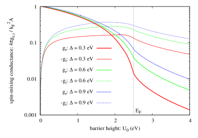
Figure 3: (Color online) $g_{r,i}$ vs. $U_{0}$ in logscale for different ${\Delta}$ values. Curves starting with values close to unity give the real part $g_{r}$, and curves starting from very low values display the imaginary part $-g_{i}$. The vertical axis is in units of the Sharvin conductance.

Appendix C Magnetization correlation for macroscopic samples

The dynamics of $\mathbf{m}$ is governed by the LLG equation:

$$\dot{\mathbf{m}}(\mathbf{r},t)=-{\gamma}\mathbf{m}(\mathbf{r},t){\times}{\bf H}_{\rm eff}+{\alpha}\mathbf{m}(\mathbf{r},t){\times}\dot{\mathbf{m}}(\mathbf{r},t),$$ (30)

where ${\bf H}_{\rm eff}=\mathbf{H}_{0}+(D/{\gamma}{\hbar}){\nabla}^{2}\mathbf{m}(\mathbf{r},t)+\mathbf{h}(\mathbf{r},t)$ is the total effective magnetic field with: (i) the external field plus the uniaxial anisotropy field $\mathbf{H}_{0}=H_{0}\hat{\mathbf{z}}=({\omega}_{0}/{\gamma})\hat{\mathbf{z}}$, (ii) the exchange field $(D/{\gamma}{\hbar}){\nabla}^{2}\mathbf{m}$ due to spatial variation of magnetization, and (iii) the thermal random fields $\mathbf{h}(\mathbf{r},t)$.

We define Fourier transforms:

$$\tilde{g}(\mathbf{k},{\omega}) ={\int}d\mathbf{r}e^{i\mathbf{k}{\cdot}\mathbf{r}}{\int}dte^{i{\omega}t}~{}g(\mathbf{r},t)$$ (31)

$$g(\mathbf{r},t) ={1\over V}{\sum}_{m,n,l}e^{-i\mathbf{k}{\cdot}\mathbf{r}}{\int}{d{\omega}\over 2{\pi}}e^{-i{\omega}t}~{}\tilde{g}(\mathbf{k},{\omega})$$ (32)

where $\mathbf{k}=2{\pi}(m/L,n/W,l/H)$ and $L,W,H$ are the length, width, and height of the ferromagnetic film. Near thermal equilibrium, $m_{\perp}{\ll}1$ (and so $m_{z}{\simeq}1$), we may linearize the LLG equation. After Fourier transformation, the linearized LLG equation becomes $\tilde{m}_{i}(\mathbf{k},{\omega})={\sum}_{j}{\chi}_{ij}(\mathbf{k},{\omega}){\gamma}\tilde{h}_{j}(\mathbf{k},{\omega})$ with $i,j=x,y$, and

$${\chi}=-{1/(1+{\alpha}^{2})\over({\omega}-{\omega}_{\mathbf{k}}^{+})({\omega}-{\omega}_{\mathbf{k}}^{-})}\left(\begin{matrix}{\omega}_{\mathbf{k}}-i{\alpha}{\omega}&-i{\omega}\\ i{\omega}&{\omega}_{\mathbf{k}}-i{\alpha}{\omega}\end{matrix}\right)$$ (33)

with ${\hbar}{\omega}_{\mathbf{k}}={\hbar}{\omega}_{0}+D|\mathbf{k}|^{2}$ and ${\omega}_{\mathbf{k}}^{\pm}={\pm}{\omega}_{\mathbf{k}}/(1{\pm}i{\alpha})$.

The spectrum of random motion in the linear response regime $x_{i}={\sum}_{j}{\chi}_{ij}f_{j}$ with “current” $x$ and random force $f$ ($x$ and $f$ are chosen such that $xf$ is in the units of energy) is comprehensively studied in Ref. Landau et al., 1980. In our problem, $f\rightarrow{\gamma}h$, $x\rightarrow(M_{s}/{\gamma})m$, ${\chi}\rightarrow(M_{s}/{\gamma}){\chi}$, the autocorrelation of the magnetization then becomes ($\bm{\zeta}=\mathbf{r}_{1}-\mathbf{r}_{2},{\tau}=t_{1}-t_{2}$)

$$\left\langle m_{i}(\bm{{\zeta}},{\tau})m_{j}(0,0)\right\rangle={2{\gamma}k_{B}T\over M_{s}V}$$

$${\times}{\sum}_{\mathbf{k}}e^{-i\mathbf{k}{\cdot}\bm{{\zeta}}}{\int}{d{\omega}\over 2{\pi}}e^{-i{\omega}{\tau}}{{\chi}_{ij}-{\chi}_{ji}^{*}\over i{\omega}}{{\hbar}|{\omega}|/k_{B}T\over e^{{\hbar}|{\omega}|/k_{\rm B}T}-1},$$ (34)

from which $\left\langle\dot{m}_{i}(\bm{{\zeta}},{\tau})m_{j}(0,0)\right\rangle$ can be caluclated by taking derivative over ${\tau}$.

The limit $\bm{{\zeta}}=0$ and ${\tau}=0$ can be obtained for three-dimensional systems by replacing the sum over $\mathbf{k}$ by an integral $V^{-1}{\sum}_{\mathbf{k}}\rightarrow{\int}d^{3}\mathbf{k}/(2{\pi})^{3}$ in Eq. (34):

$$\left\langle m_{i}(0,0)m_{j}(0,0)\right\rangle =Z_{3\over 2}{{\gamma}{\hbar}\over M_{s}}\left(k_{\rm B}T\over 4{\pi}D\right)^{3\over 2}{\delta}_{ij},$$ (35)

$$\left\langle\dot{m}_{i}(0,0)m_{j}(0,0)\right\rangle ={3Z_{5\over 2}{\gamma}k_{B}T\over 2M_{s}}\left(k_{\rm B}T\over 4{\pi}D\right)^{3\over 2}\left(\begin{matrix}-{\alpha}&-1\\ 1&-{\alpha}\end{matrix}\right)_{ij},$$ (36)

where $Z$ is the Zeta function.

Appendix D Relation between ${\alpha}$ and ${\tau}_{mp}$

Here we derive a relationship between the magnetic damping constant ${\alpha}$ and the magnon-phonon thermalization time ${\tau}_{mp}$. When the magnon and phonon temperatures are $T_{m}$ and $T_{p}$, the magnon-phonon relaxation time is phenomenologically defined by: Sanders and Walton (1977)

$${d\over dt}(T_{p}-T_{m})=-{T_{p}-T_{m}\over{\tau}_{mp}}.$$ (37)

If the phonon system is attached to a huge reservoir (substrate) such that its temperature $T_{p}$ is fixed ($dT_{p}/dt=0$), Eq. (37) becomes

$${dT_{m}\over dt}{\simeq}-{T_{m}-T_{p}\over{\tau}_{mp}}.$$ (38)

In metals we should consider three subsystems (magnon, phonon, electron) leading to

$${dT_{s}\over dt}=-{\sum}_{t}k_{st}(T_{s}-T_{t}),$$ (39)

with $s,t=$ m, p, e for magnon, phonon, and electron. The coupling strength $k_{st}={\tau}_{st}^{-1}C_{t}/(C_{s}+C_{t})$ with the $s$-$t$ relaxation time ${\tau}_{st}$ and the specific heat $C_{s}$. When the magnon specific heat is much less than that of phonons and electrons ($C_{m}{\ll}C_{p},C_{e}$)

$${dT_{m}\over dt}{\simeq}-{T_{m}-T_{p}\over{\tau}_{mp}}-{T_{m}-T_{e}\over{\tau}_{me}}.$$ (40)

We may parameterize the magnon temperature by the thermal suppression of the average magnetization:

$$H_{\rm eff}M_{s}V(1-\langle m_{z}\rangle)=k_{B}T_{m},$$ (41)

where $H_{\rm eff}$ points in the $\hat{\mathbf{z}}$-direction. The LLG equation provides us with the information about $m_{z}$:

$$\dot{\mathbf{m}}=-{\gamma}\mathbf{m}{\times}({\bf H}_{\rm eff}+\mathbf{h})+{\alpha}~{}\mathbf{m}{\times}\dot{\mathbf{m}},$$ (42)

where the random thermal field $\mathbf{h}=\mathbf{h}_{p}+\mathbf{h}_{e}$ from the lattice and electrons are determined by the phonon/electron temperature:

$$\langle{\gamma}h_{p/e}^{i}(t){\gamma}h_{p/e}^{j}(0)\rangle={2{\gamma}{\alpha}_{p/e}k_{B}T_{p/e}\over M_{s}V}$$ (43)

with ${\alpha}_{p/e}$ the magnetic damping caused by scattering with phonons/electrons and ${\alpha}={\alpha}_{p}+{\alpha}_{e}$. Therefore

$$-{k_{B}\over H_{\rm eff}M_{s}V}{dT_{m}\over dt}=\langle\dot{m}_{z}\rangle=\langle m_{y}{\gamma}h_{x}-m_{x}{\gamma}h_{y}\rangle+{\alpha}\langle m_{x}\dot{m}_{y}-m_{y}\dot{m}_{x}\rangle={1\over 1+{\alpha}^{2}}{2{\gamma}k_{B}({\alpha}T_{m}-{\alpha}_{p}T_{p}-{\alpha}_{e}T_{e})\over M_{s}V},$$ (44)

or

$${dT_{m}\over dt}=-{2{\omega}_{0}\over 1+{\alpha}^{2}}({\alpha}T_{m}-{\alpha}_{p}T_{p}-{\alpha}_{e}T_{e}),$$ (45)

with ${\omega}_{0}={\gamma}H_{\rm eff}$. Comparing Eq. (45) with Eq. (40), we find

$$2{\alpha}{\omega}_{0}{\simeq}{2{\alpha}{\omega}_{0}\over 1+{\alpha}^{2}}={2{\alpha}_{p}{\omega}_{0}\over 1+{\alpha}^{2}}+{2{\alpha}_{e}{\omega}_{0}\over 1+{\alpha}^{2}}={1\over{\tau}_{mp}}+{1\over{\tau}_{me}}.$$ (46)

For the ferromagnetic insulator YIG: ${\alpha}{\simeq}6.7{\times}10^{-5}$ and ${\omega}_{0}{\simeq}10$ GHz (Ref. Kajiwara et al., 2010), thus ${\tau}_{mp}=1/2{\alpha}{\omega}_{0}{\simeq}10^{-6}$ s, which agrees with ${\tau}_{mp}{\simeq}10^{-6}$ s in Ref. Sanders and Walton, 1977.

The estimate above relies on the macrospin approximation. Considering magnons from all $\mathbf{k}$ adds a prefactor of order of unity.

References

- (1) Spin Caloritronics, Special Issue of Sol. Stat. Commun. (G.E.W. Bauer, A.H. MacDonald, and S. Maekawa, eds), 150, 459 (2010).
- Uchida et al. (2008) K. Uchida, S. Takahashi, K. Harii, J. Ieda, W. Koshibae, K. Ando, S. Maekawa, and E. Saitoh, Nature 455, 778 (2008); Sol. Stat. Commun. 150, 524 (2010).
- Valenzuela and Tinkham (2006) S. O. Valenzuela and M. Tinkham, Nature 442, 176 (2006).
- Kimura et al. (2007) T. Kimura, Y. Otani, T. Sato, S. Takahashi, and S. Maekawa, Phys. Rev. Lett. 98, 156601 (2007).
- (5) M. Hatami, G. E. W. Bauer, S. Takahashi, and S. Maekawa, Sol. Stat. Commun. 150, 480 (2010).
- Sanders and Walton (1977) D. J. Sanders and D. Walton, Phys. Rev. B 15, 1489 (1977).
- Kittel and Abrahams (1953) C. Kittel and E. Abrahams, Rev. Mod. Phys. 25, 233 (1953).
- Beaurepaire et al. (1996) E. Beaurepaire, J. Merle, A. Daunois, and J. Bigot, Phys. Rev. Lett. 76, 4250 (1996).
- Tserkovnyak et al. (2002) Y. Tserkovnyak, A. Brataas, and G. E. W. Bauer, Phys. Rev. Lett. 88, 117601 (2002).
- Foros et al. (2005) J. Foros, A. Brataas, Y. Tserkovnyak, and G. E. W. Bauer, Phys. Rev. Lett. 95, 016601 (2005).
- Xiao et al. (2009) J. Xiao, G. E. W. Bauer, S. Maekawa, and A. Brataas, Phys. Rev. B 79, 174415 (2009).
- Yelon and Berger (1972) W. B. Yelon and L. Berger, Phys. Rev. B 6, 1974 (1972).
- Demokritov et al. (2006) S. O. Demokritov, V. E. Demidov, O. Dzyapko, G. A. Melkov, A. A. Serga, B. Hillebrands, and A. N. Slavin, Nature 443, 430 (2006).
- (14) http://www.isowave.com/pdf/materials/Yttrium_Iron_Garnet.pdf.
- Shinozaki (1961) S. S. Shinozaki, Phys. Rev. 122, 388 (1961).
- (16) E. G. Spencer and R. C. LeCraw, Phys. Rev. Lett. 4, 130 (1960).
- Kajiwara et al. (2010) Y. Kajiwara, K. Harii, S. Takahashi, J. Ohe, K. Uchida, M. Mizuguchi, H. Umezawa, H. Kawai, K. Ando, K. Takanashi, S. Maekawa, and E. Saitoh, Nature 464, 262 (2010).
- (18) K. Uchida, J. Xiao, H. Adachi, J. Ohe, S. Takahashi, J. Ieda, T. Ota, Y. Kajiwara, H. Umezawa, H. Kawai, G. E. W. Bauer, S. Maekawa, E. Saitoh, Nature Materials (in press).
- Roy et al. (2009) P. E. Roy, J. H. Lee, T. Trypiniotis, D. Anderson, G. A. C. Jones, D. Tse, and C. H. W. Barnes, Phys. Rev. B 79, 060407 (2009).
- Vlaminck and Bailleul (2008) V. Vlaminck and M. Bailleul, Science 322, 410 (2008).
- Hsu and Berger (1976) Y. Hsu and L. Berger, Phys. Rev. B 14, 4059 (1976).
- Brataas et al. (2006) A. Brataas, G. E. W. Bauer, and P. J. Kelly, Physics Reports 427, 157 (2006).
- Takahashi and Maekawa (2008) S. Takahashi and S. Maekawa, Science and Technology of Advanced Materials 9, 014105 (2008).
- Jin et al. (2006) D. Jin, Y. Ren, Z. zhong Li, M. wen Xiao, G. Jin, and A. Hu, in J. Appl. Phys. 99, 08T304–3 (2006).
- Landau et al. (1980) L. D. Landau, E. M. Lifsic, L. P. Pitaevskii, J. Sykes, and M. J. Kearsley, Statistical physics Vol. 9 (Butterworth-Heinemann, 1980).