Sustaining the Internet with hyperbolic mapping

Abstract

The Internet infrastructure is severely stressed. Rapidly growing overheads associated with the primary function of the Internet—routing information packets between any two computers in the world—cause concerns among Internet experts that the existing Internet routing architecture may not sustain even another decade. Here we present a method to map the Internet to a hyperbolic space. Guided with the constructed map, which we release with this paper, Internet routing exhibits scaling properties close to theoretically best possible, thus resolving serious scaling limitations that the Internet faces today. Besides this immediate practical viability, our network mapping method can provide a different perspective on the community structure in complex networks.

I Introduction

In the Information Age, the Internet is becoming a de facto public good, akin to roads, airports, or any other critical infrastructure Gehring (2004). More than a billion people are estimated to use the Internet every day to communicate, search for information, share data, or do business Internet World Stats . On-line social networks are becoming an integral part of human social activities, increasingly affecting human psychology Lazer et al. (2009). Underlying all these processes is the Internet infrastructure, composed, at the large scale, of connections between Autonomous Systems (ASs). An AS is, roughly, a part of the Internet owned and administered by the same organisation Hawkinson and Bates (1996). ASs range in size from small companies, or even private users, to huge international corporations. There is no central Internet authority dictating to any AS what other ASs to connect to. Connections between ASs are results of local independent decisions based on business agreements between AS pairs. This lack of centralised engineering control makes the Internet a truly self-organised system, and poses many scientific challenges. The one we address here is the sustainability of Internet growth.

The Internet has been growing fast according to all measures Dhamdhere and Dovrolis (2008); Carpenter (2009). For example, the number of ASs increases by approximately $2,400$ every year Dhamdhere and Dovrolis (2008). Despite its growth, the Internet must sustainably perform its primary task—routing information packets between any two computers in the world. But can this function be really sustained? To route information to a given destination in the Internet today, all ASs must collectively discover the best path to each possible destination, based on the current state of the global Internet topology. As the number of destinations grows quickly, the amount of information each AS has to maintain becomes a serious scalability concern, endangering the performance and stability of the Internet Meyer et al. (2007). Worse yet, the Internet is not static. Its topology changes constantly due to failures of existing links and nodes, or appearances of new ones. Each time such a change occurs anywhere in the Internet, the information about this event must be diffused to all ASs, which have to quickly process it to recompute new best routes. The constantly increasing size and dynamics of the Internet thus leads to immense and quickly growing routing overheads, causing concerns among Internet experts that the existing Internet routing architecture may not sustain even another decade Meyer et al. (2007); Atkinson and Bennett (2009); Godfrey et al. (2009); Gammon (2010); parts of the Internet have started sinking into black holes already Katz-Bassett et al. (2008).

The scaling limitations with existing Internet routing stem from the requirement to have a current state of the Internet topology distributed globally. Such global knowledge is unavoidable since routing has no source of information other than the network topology. Routing in these conditions is equivalent to routing using a hypothetical road atlas, which has no geographic information, but just lists road network links, which are pairs of connected road intersections, abstractly identified. This analogy with road routing suggests that there are better ways to find paths in networks. Suppose we want to travel from one geographic place to another. Given the geographic coordinates of our starting point and destination, we can readily tell what direction brings us closer to our destination. We see that a coordinate system in a geometric space, coupled with a representation of the world in this space, simplify drastically our routing task. For simple and efficient network routing we thus need a map. Constructing such a map for the Internet boils down to assigning to each AS its coordinates in some geometric space, and then using this space to forward information packets in the right directions toward their destinations. Greedy forwarding implements this routing in the right direction: upon reading the destination address in the packet, the current packet holder forwards the packet to its neighbour closest to the destination in the space. This greedy strategy to reach a destination is efficient only if the network map is congruent with the network topology. In the analogy with road routing, for example, this congruency condition means that there should exists a road path that stays approximately close to the geographic geodesic between the trip’s starting and ending points. If the congruency condition holds, then the advantage of greedy forwarding is twofold. First, the only information that ASs must maintain is the coordinates of their neighbours. That is, ASs do not have to keep any per-destination information. Second, once ASs are given their coordinates, these coordinates do not change upon topological changes of the Internet. Therefore, ASs do not have to exchange any information about ever-changing Internet topology. Taken together, these two improvements essentially eliminate the two scaling limitations mentioned above.

In our recent work Boguñá et al. (2009); Boguñá and Krioukov (2009); Krioukov et al. (2009a); Papadopoulos et al. (2010) we have shown that greedy forwarding is indeed efficient in Internet-like synthetic networks embedded in geometric spaces, and that this efficiency is maximised if the space is hyperbolic. However, putting these ideas in practice needs a crucial piece of information: a map of the real Internet in a hyperbolic space. Here we present a method to find such a map.

Our method uses statistical inference techniques to find coordinates for each AS in the hyperbolic space underlying the Internet. Guided by the inferred coordinates, greedy forwarding in the Internet achieves efficiency and robustness, similar to those in synthetic networks. We also find that the method maps geo-politically close ASs close to each other in the hyperbolic space. This finding suggests that our mapping method can be used for soft community detection in real networks, where by soft communities we mean groups of geometrically close nodes.

II The model

To build a geographic map, one first has to model the Earth surface, e.g., by assuming that it is a sphere. Similarly, we also need a geometric model of the Internet space to build our map. The simplest candidate space is also a sphere, or even a circle, on which nodes are uniformly distributed, and connected by an edge with probability $p(d)$ decreasing as a function of distance $d$ between nodes, conceptually similar to random geometric graphs Penrose (2003). However, this model fails to capture basic properties of the Internet topology, including its scale-free node degree distribution. In Serrano et al. (2008), we showed that to generate realistic network topologies in this geometric approach, we first have to assign to nodes their expected degrees $\kappa$ drawn from a power-law distribution, and then connect pairs of nodes with expected degrees $\kappa$ and $\kappa^{\prime}$ with probability $p(\chi)$, where $\chi$ is distance $d$ rescaled by the product of the expected degrees, $\chi\sim d/(\kappa\kappa^{\prime})$. We thus have a hybrid model that mixes geometry and topology—geometric characteristics, distances $d$ used in random geometric graphs, come in tandem with topological characteristics, expected degrees $\kappa$ used in classical configuration models of random power-law graphs Chung and Lu (2002). If we associate the expected degree $\kappa$ of a node with its mass, then the connection probability $p(d/(\kappa\kappa^{\prime}))$, which is a measure of the interaction strength between two nodes, resembles Newton’s law of gravitation. Therefore we call this model Newtonian. However, according to Einstein, we can treat gravity in purely geometric terms if we accept that the space is no longer flat, i.e., if it is non-Euclidean. Following this philosophy we showed in Krioukov et al. (2009b); Krioukov et al. (2010) that the Newtonian model is isomorphic to a purely geometric network model with node degrees transformed into a geometric coordinate making the space hyperbolic, i.e., negatively curved. We call this model Einsteinian.

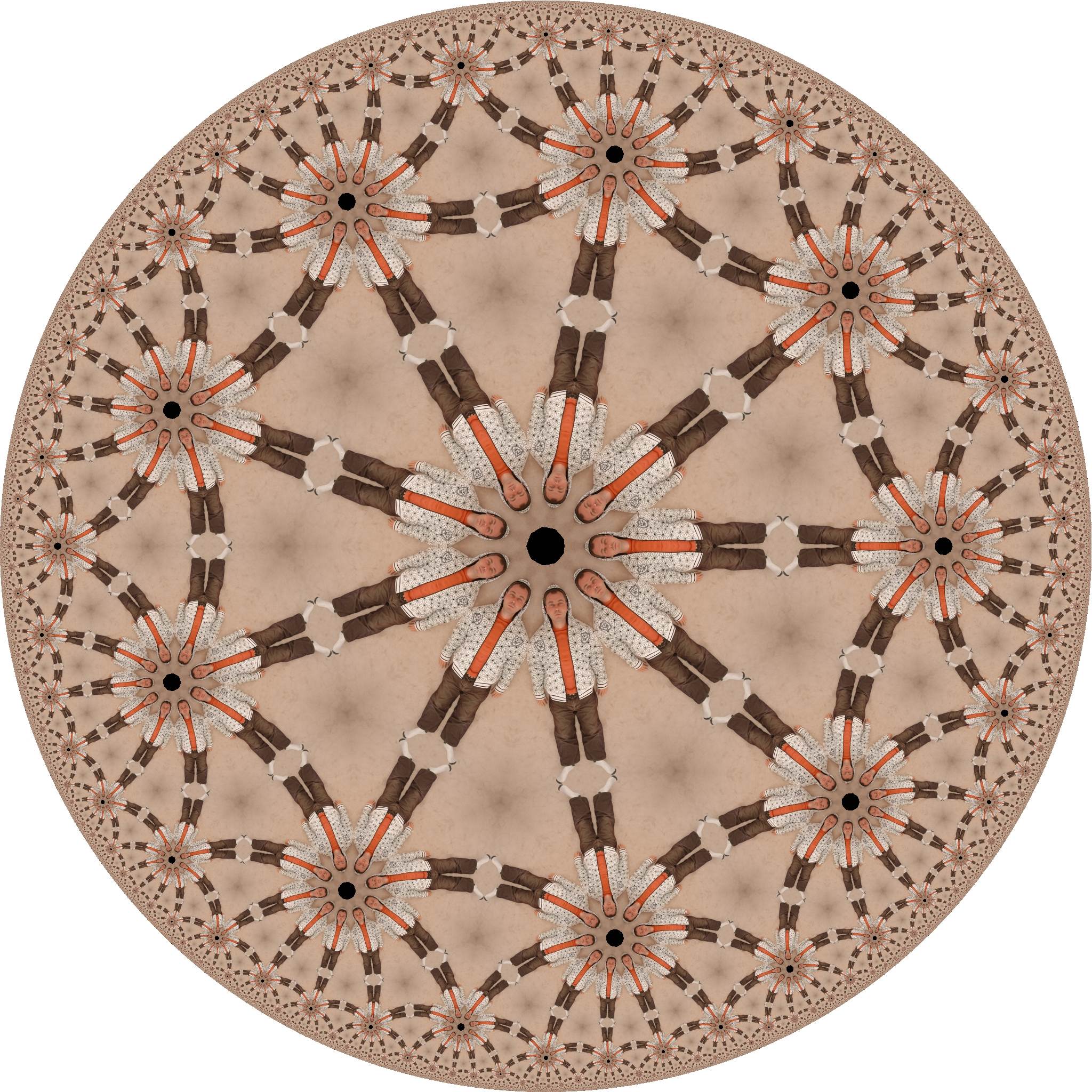
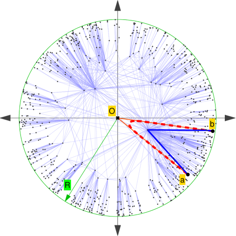
The main property of hyperbolic geometry is the exponential expansion of space illustrated in Fig. 1. For example, the area $A(r)$ of a two-dimensional hyperbolic disc of radius $r$ grows with $r$ as $A(r)\sim e^{r}$. Consequently, if we distribute nodes uniformly or quasi-uniformly over a hyperbolic disc, then from the Euclidean perspective their density will grow exponentially with the distance from the disc centre. We illustrate this effect in Fig. 2, where we visualise a small-size sample network generated by our Einsteinian model. In the model, nodes are indeed distributed (quasi-)uniformly within a hyperbolic disc of radius $R$, which is a function of the network size. We see that the angular node density appears uniform, but the radial one does not—the number of nodes grows exponentially as we move away from the origin. The figure also shows a triangle connecting origin $O$, and two nodes $a$ and $b$ by hyperbolic geodesics, i.e., hyperbolically straight lines. The two geodesics emanating from the origin $O$, $\overline{Oa}$ and $\overline{Ob}$, are radial straight lines, and their hyperbolic lengths $x$ are equal to the radial coordinates of $a$ and $b$: $x_{Oa}=r_{a}$ and $x_{Ob}=r_{b}$. However, the hyperbolic geodesic between nodes $a$ and $b$ does not appear as a Euclidean straight line, and its length is given by the hyperbolic law of cosines

$$\cosh x_{ab}=\cosh r_{a}\cosh r_{b}-\sinh r_{a}\sinh r_{b}\cos\Delta\theta_{ab},$$ (1)

where $\Delta\theta_{ab}$ is the angle between $\overline{Oa}$ and $\overline{Ob}$. (The same formula with $r_{O}=0$ can be used to compute $x_{Oa}=r_{a}$ and $x_{Ob}=r_{b}$.) Upon distributing nodes over the disc as described, we form scale-free networks in the model by connecting each pair of nodes $i$ and $j$ located at hyperbolic distance $x_{ij}$ with the connection probability

$$p(x_{ij})=\left(1+e^{\frac{x_{ij}-R}{2T}}\right)^{-1},$$ (2)

almost identical to the Fermi-Dirac distribution in statistical mechanics. It depends only on hyperbolic distances $x_{ij}$ (link energies), hyperbolic disc radius $R$ (chemical potential), and parameter $T\geqslant 0$ (temperature) controlling network clustering. This connection probability results in average node degrees exponentially decreasing with the distance from the origin, which we also observe in Fig. 2. The combination of an exponentially increasing node density and exponentially decreasing average degree yields a power-law node degree distribution in the network. See Appendix A for further details.

Figure 1: The exponentially growing number of people lying on the hyperbolic floor illustrates the exponential expansion of hyperbolic space. All people are of the same hyperbolic size. The Poincaré tool developed by Bill Horn is used to construct the tessellation of the hyperbolic plane in the Poincaré disc model with the Schläfli symbol $\{9,3\}$, rendering an image of the last author.

Figure 2: Connection between hyperbolic geometry and scale-free topology of complex networks illustrated by a synthetic network in the Einsteinian model. All nodes lie within a hyperbolic disc of radius $R$. The radial density of nodes grows exponentially with the distance from the origin $O$, while their average degree exponentially decreases, yielding a scale-free degree distribution. The red lines show triangle $Oab$ made of the hyperbolic geodesics connecting origin $O$ and two nodes $a$ and $b$. Geodesics $\overline{Oa}$ and $\overline{Ob}$ are the solid lines, while geodesic $\overline{ab}$ is the dashed curve. The thick blue links show the shortest path between nodes $a$ and $b$ in the network.

III The mapping method

As our goal is to build a realistic Internet map, ready for routing and other applications, we have to find for each AS its radial and angular coordinates $(r,\theta)$ maximising the efficiency of greedy forwarding. This specific task of maximising greedy forwarding efficiency calls for a mapping method different from existing techniques on embedding Internet distances and graphs Tang and Crovella (2003); Shavitt and Tankel (2004, 2008). In view of our previous findings Boguñá et al. (2009); Boguñá and Krioukov (2009); Krioukov et al. (2009a); Papadopoulos et al. (2010) that greedy forwarding is exceptionally efficient in Internet-resembling synthetic networks, and that this efficiency is maximised in the Einsteinian model, our strategy for the Internet map construction is to maximise the congruency between the map and the model. In statistical inference Cox (2006), this goal is equivalent to maximising the likelihood that the observed data, i.e., the Internet topology, has been produced by the model. This likelihood is given by

$${\cal L}=\prod_{i<j}p(x_{ij})^{a_{ij}}[1-p(x_{ij})]^{1-a_{ij}},$$ (3)

where the elements $a_{ij}$ of the Internet adjacency matrix are equal to $1$ whenever there exists a connection between ASs $i$ and $j$, and to $0$ otherwise. While the adjacency matrix represents the observed data, the connection probability $p(x_{ij})$ depends via Eqs. (2,1) on the AS coordinates $(r,\theta)$, which we try to infer. Our best estimate for these coordinates are then those maximising the likelihood in Eq. (3).

Figure 3: The hyperbolic map of the Internet is similar to a synthetic Einsteinian network in Fig. 2. The size of AS nodes is proportional to the logarithm of their degrees. For the sake of clarity, only ASs with degree above $3$, and only the connections with probability $p(x)>0.5$ given by Eq. (2) are shown. The font size of the country names is proportional to the logarithm of the number of ASs that the country has. Only the names of countries with more than $10$ ASs are included. The methods used to map ASs to their countries are described in Appendix D.

Although there are a plenty of methods to find maximum-likelihood solutions, e.g., the Metropolis-Hastings algorithm Newman and Barkema (1999), they perform poorly and do not scale well on large datasets with abundant local maxima, which is the case with the Internet. Therefore, as important as a maximisation method is a heuristic approach helping the maximisation algorithm to find the optimal solution in a reasonable amount of time and with reasonable computational resources. Our method is based on the following remarkable property of networks in our model; the same property holds for the Internet Serrano et al. (2008). Let ${\cal G}$ be a given network with average degree $\bar{k}$ and power-law degree distribution $P(k)\sim k^{-\gamma}$, and let ${\cal G}(k_{T})$ be ${\cal G}$’s subgraph composed of nodes with degree larger than some threshold $k_{T}$, along with the connections among these nodes. The average degree in ${\cal G}(k_{T})$ is then given by $\bar{k}(k_{T})=k_{T}^{3-\gamma}\bar{k}$ Serrano et al. (2008). In scale-free networks with exponent $\gamma$ between $2$ and $3$, this internal average degree is thus a growing function of $k_{T}$, which implies that subgraphs made of high degree nodes almost surely form a single connected component. Using this property along with the statistical independence of the graph edges, it becomes possible to infer coordinates of ASs in ${\cal G}(k_{T})$ ignoring the remainder of the AS graph. This property is practically important because the size of ${\cal G}(k_{T})$ decreases very fast as $k_{T}$ increases, which speeds up likelihood maximisation algorithms tremendously. In a nutshell, our method starts with a subgraph ${\cal G}(k_{T})$ small enough for standard maximisation algorithms being able to reliably and quickly infer the coordinates of ASs in ${\cal G}(k_{T})$. Once these are found, we gradually increase $k_{T}$ to iteratively add layers of lower-degree ASs. While doing so, we use the already inferred AS coordinates as a reference frame to assign initial coordinates to newly added ASs. This initial coordinate assignment significantly improves the convergence time of maximisation algorithms. All other details of our mapping method can be found in Appendix B.

IV Mapping results

Figure 4: Hyperbolic mapping of the Internet is successful, as the empirical connection probability between ASs of degree larger than $2$ in the map closely follows the Einsteinian model prediction. The whole range of hyperbolic distances $x\in[0,2R]$ is binned, and for each bin the ratio of the number of connected AS pairs to the total number of AS pairs falling within this bin is shown. The distances between AS pairs are computed using Eq. (1). The blue dashed line is the connection probability given by Eq. (2) with $R=27$ and $T=0.69$, which are the values used by the mapping method.

Figure 5: Hyperbolic mapping of the Internet yields meaningful results, as ASs belonging to the same country are mapped close to each other. The angular distributions of ASs in the thirty largest countries in the world are shown. The “size” of the country is the number of ASs it has. The graph shows the percentage of ASs per bin of size $3.6^{o}$. For the majority of countries, their ASs are localised in narrow regions. The exceptions are the US, EU, and UK. The first two exceptions are due the significant geographic spread of ASs belonging to the US or EU, the latter actually representing not one country but a collection of countries.

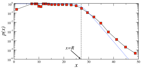
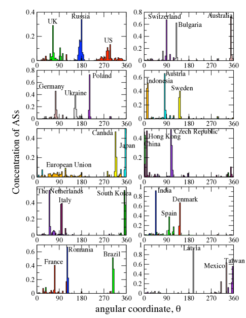
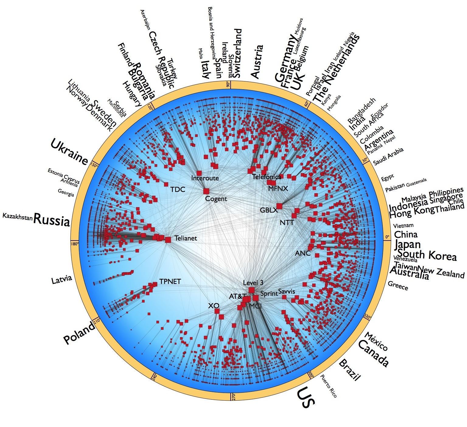
We apply our mapping method to the Internet AS topology extracted from the Archipelago project data Claffy et al. (2009) in June 2009 and described in Appendix C, and visualise the results in Fig. 3. We observe striking similarity between this visualisation and the synthetic Einsteinian network in Fig. 2. To confirm that the Internet map we have obtained is indeed congruent with the Einsteinian model, we juxtapose in Fig. 4 the empirical connection probability between ASs in the obtained Internet map against the theoretical one in Eq. (2). We observe a clear similarity between the two. Neither the sphere is a perfect model of the Earth, nor the Einsteinian model is an ideal abstraction of the Internet structure. Yet, the observed similarity between the empirical and theoretical connection probabilities in Fig. 4 suggests that hyperbolic metric spaces coupled with Fermi-like connection probabilities are reasonable representations of the real Internet space.

To investigate further the connections between the obtained map and Internet reality, we show in Fig. 3 the average angular position of all ASs belonging to the same country, while in Fig. 5 we draw the angular distributions of those ASs. Surprisingly, we find that even though our mapping method is completely geography-agnostic, it discovers meaningful groups or communities of ASs belonging to the same country. Furthermore, in Fig. 3 we find many cases of geographically or politically close countries placed close to each other in our hyperbolic map. The explanation of these surprising effects is rooted in the peculiar nature of our mapping method. If ASs belonging to the same country, geographic region, or geo-political or economic group are connected more densely to each other than to the rest of the world, then this higher connection density translates to a higher attractive force that tries to place all such ASs close to each other in our map. Indeed, the term $p(x_{ij})^{a_{ij}}$ in Eq. (3) corresponds to the attractive force between connected nodes, while the term $[1-p(x_{ij})]^{1-a_{ij}}$ is the repulsive force between disconnected ones. This peculiar interplay between attraction within densely connected regions, and repulsion across sparsely connected zones, effectively maps closely the ASs belonging to densely connected AS groups. These observations build our confidence that our mapping method provides meaningful results reflecting peculiarities of the real Internet structure, and suggest that the method can be adapted to discover the community structure Girvan and Newman (2002); Newman (2006); Danon et al. (2007) in other complex networks.

V Routing results

The obtained Internet map is ready for greedy forwarding. An AS holding a packet reads its destination AS coordinates, computes the hyperbolic distances between this destination and each of its AS neighbours using Eq. (1), and forwards the packet to the neighbour closest to the destination. To evaluate the performance of this process, we perform greedy forwarding from each source to each destination AS, and compute several performance metrics.

The first metric is success ratio, which is the percentage of greedy paths that successfully reach their destinations. Not all paths are expected to be successful as some might run into local minima. For example, an AS might forward a packet to its neighbour who sends the packet back to the same AS, in which case the packet will never reach the destination. We declare a path unsuccessful, if the packet is sent to the same AS twice. The average success ratio of simple greedy forwarding in our Internet map is remarkably high, $97\%$, and more sophisticated greedy forwarding techniques, such as those described in Cvetkovski and Crovella (2009), can boost it to $100\%$.

Given the discussed connections between our Internet map and geography, one may conjecture that greedy forwarding simply mimics geographic routing following the geographically shortest paths. However, this conjecture is not true. Geography is reflected in our map only along the angular coordinate, while the radial coordinate is a function of the AS degree, making the space hyperbolic, see Appendix A. The geographic space is not hyperbolic, and if we use it for greedy forwarding, we obtain a much lower success ratio of approximately $14\%$. We also tested modified geographic routing that tries to intelligently use AS degrees, in spirit of our Einsteinian model. Nevertheless, this modification, although improving the success ratio to $30\%$, still fails short compared to the results obtained using our hyperbolic map. The details of these experiments with geographic routing are in Appendix E.

The second metric is stretch, which tells us by how much longer the greedy paths are, compared to shortest paths in the Internet topology. The average stretch is low, $1.1$. The average hop-wise length of the shortest paths between selected sources and destinations is $3.49$, so that the average length of greedy paths is $3.86$. The low value of stretch indicates that greedy paths are close to optimal, i.e., shortest paths. The shortest path between nodes $a$ and $b$ in Fig. 2, for example, is also the path found by greedy forwarding. Somewhat unexpectedly, the greedy stretch is asymptotically optimal, i.e., equal to $1$, in scale-free, strongly clustered networks regardless what underlying space is used for greedy forwarding Boguñá and Krioukov (2009). Low stretch also implies that greedy forwarding causes approximately the same traffic load on nodes as shortest-path forwarding. Given that shortest-path forwarding does not lead to high traffic load in scale-free networks Gkantsidis et al. (2003), this finding allays concerns that hyperbolic forwarding may cause traffic congestion abnormalities Jonckheere et al. (2010). More details on this topic are in Appendix F.

Figure 6: Greedy forwarding performs almost optimally in the mapped Internet, as indicated by the success ratio, $p_{s}$, and average stretch, $\bar{s}$, after removal of a given fraction of AS nodes (top left) or links (top right). The bottom plots show these two metrics after removing a number of the highest-degree nodes (bottom left), and a fraction of links among highest-degree nodes (bottom right). The links are first ranked by the product of node degrees that they connect, and then a fraction of top-ranked links are removed. The giant connected component is still present after all removals, but it drops to $85\%$ of the original graph after the removal of $10$ hubs.

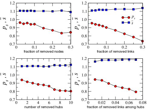
The two metrics above characterise the performance of greedy forwarding in the static Internet topology. More important than that is how greedy forwarding performs in the dynamic topology, where links and nodes can fail. We randomly select a percentage of links and nodes, remove them from the mapped Internet, recompute the success ratio and stretch after the removal, and present the result in the top plots of Fig. 6. Even upon simultaneous failures of up to $10\%$ of AS links or nodes—catastrophic events never happened in the Internet history—we observe only minor degradation of the performance of greedy forwarding. That is, even catastrophic levels of damage to the Internet does not significantly affect the performance of greedy forwarding, even though no AS changes its position on the hyperbolic map.

A widely popularized feature of complex networks is their robustness with respect to random failures, and the lethality of failures of highest-degree hubs Albert et al. (2001); Jeong et al. (2001). As expected we observe in the bottom plots of Fig. 6 that removals of such hubs have a more detrimental effect on greedy forwarding as well. However, targeted removal of highest-degree ASs in the Internet is a rather unrealistic scenario since these large ASs consist of thousands of routers whose simultaneous failure is a very rare and unlikely event. The explanation for the surprising efficiency of greedy forwarding with respect to random failures lies in the unique combination of the following two properties exhibited by scale-free, strongly clustered networks: high path diversity Gkantsidis et al. (2003), and congruency between hyperbolic geodesics and topologically shortest paths Papadopoulos et al. (2010); Krioukov et al. (2009b); Krioukov et al. (2010). The latter is illustrated by the similar path patterns of the hyperbolic geodesic and topologically shortest path between nodes $a$ and $b$ in Fig. 2: they both first go to the high-degree core of the network, and then exit it in the appropriate direction to the destination. Due to high path diversity, there are many disjoint shortest paths between the same source and destination, and thanks to the congruency, they all stay close to the corresponding hyperbolic geodesics. Link and node failures affect some shortest paths, but others remain, and greedy forwarding can still find them using the same hyperbolic map.

Another form of Internet dynamics is its rapid growth over years Dhamdhere and Dovrolis (2008); Carpenter (2009); Pastor-Satorras and Vespignani (2004); Crovella and Krishnamurthy (2006). We show in Appendix G that if the existing ASs keep their hyperbolic coordinates fixed, while the ASs joining the Internet anew compute their coordinates using local information, then the performance of greedy forwarding does not significantly degrade, even at long time scales. In a nutshell, the existing AS coordinates are essentially static, as they can stay the same for years.

Existing Internet topology measurements including the Archipelago data Claffy et al. (2009) are known to be incomplete and miss some AS links. Therefore a natural question is how this missing information affects the quality of the constructed map, and the performance of greedy forwarding in it. Intuitively, since the performance of greedy forwarding is robust with respect to link removals, then we might expect it to be robust with respect to missing links as well. Moreover, if the constructed map is used in practice, then greedy forwarding will see and use those links that topology measurements do not see. We might thus also intuitively expect greedy forwarding to perform better in practice than we report in this section, simply because those missing links, when used by greedy forwarding, would provide additional shortcuts between potentially remote ASs. We confirm this intuition in Appendix H with experiments emulating the missing link issue. Therefore the routing results reported here should actually be considered as lower bounds for greedy routing performance that can be achieved in practice using the constructed hyperbolic Internet map.

VI Conclusion

We have constructed a hyperbolic map of the Internet, and release this map with this paper BoP . The map can be used for essentially infinitely scalable Internet routing. The amount of routing information that ASs must maintain is proportional to the AS degree, which is theoretically best possible since ASs must always keep some information about their neighbours. Routing communication overheads are also minimised, since ASs do not exchange any routing information upon dynamic changes of the AS topology. The presented solution thus achieves routing efficiency close to theoretically optimal, and resolves serious scaling limitations that the Internet faces today.

The mapping method we have employed is generic, and can be applied to other complex networks with underlying metric structures and heterogeneous degree distributions. We showed in Serrano et al. (2008) that a good indicator for the presence of an underlying metric structure is self-similarity of clustering in the network, while in Krioukov et al. (2009b); Krioukov et al. (2010) we showed that as soon as a metric space is present, and the network has a heterogeneous degree distribution, the metric distances can be rescaled such that the underlying geometry is effectively hyperbolic. Roughly, self-similar clustering is responsible for the metric structure along the angular coordinate, while degree heterogeneity adds the radial dimension, and makes the space hyperbolic. Applied to other networks, our mapping method can provide a different perspective on the community structure in networks. Instead of trying to split nodes into discrete community sets Girvan and Newman (2002); Newman (2006); Danon et al. (2007), it would naturally yield a continuous measure of similarity between nodes based on hyperbolic distances. More similar nodes would be located closer to each other, and form zones of higher connectivity density. It would be then up to an experimenter to define communities, if needed, as histograms of the node density in the hyperbolic space. The spectrum of potential applications of this network-mapping geometrisation agenda is wide. Network mapping can reveal geometric forces effectively driving information signaling in the network; examples include the brain Bullmore and Sporns (2009) and cell signaling networks Charlebois (2009). One can then potentially predict what network perturbations drive these networks to failures, such as brain disorders or cancer. Other applications range from recommender systems Monroe (2009), where to have the right measure of similarity between consumers is a key, to epidemic spreading Meloni et al. (2009) and information theory of networks Bianconi et al. (2009).

We have shown that the Internet hyperbolic map is remarkably robust with respect to even substantial perturbations of the Internet topology, implying that this map is essentially static. It does not significantly depend on topology dynamics, and can thus be computed only once. This property is desirable in view of long running times intrinsic to likelihood maximisation algorithms. Our method improves their running times drastically, and the Internet map computations take approximately a day on a modern computer. However, for substantially larger networks the running times may still be prohibitive even for one-time mapping. Therefore, alternative methods for network mapping, not relying on likelihood maximisation, are highly desirable, and our work in this direction is underway.

Appendix A The Einsteinian and Newtonian models of complex networks

To synthesise a network with our Einsteinian model, one has first to specify any desired network size $N$, average degree $\bar{k}$, average clustering $\bar{C}$, and exponent $\gamma>2$ of the power-law distribution $P(k)$ of node degrees $k$, $P(k)\sim k^{-\gamma}$. Equipped with these target properties of the network topology, we first distribute quasi-uniformly $N$ nodes within a hyperbolic disc of radius $R=2\log(N/c)$, where $c$ is given by

$$c=\bar{k}\frac{\sin\pi T}{2T}\left(\frac{\gamma-2}{\gamma-1}\right)^{2},$$ (4)

and $T\in[0,1]$ is a function of $\bar{C}$. In the hyperbolic plane, the quasi-uniform node density means that the node angular coordinates $\theta\in[0,2\pi]$ are distributed uniformly, while their radial coordinates $r\in[0,R]$ are distributed with density

$$\rho(r)=\alpha e^{\alpha(r-R)},$$ (5)

where $\alpha=(\gamma-1)/2$. Once all nodes are in place specified by their assigned coordinates, the hyperbolic distance $x_{ij}$ between each pair of nodes $i$ and $j$ located at $(r_{i},\theta_{i})$ and $(r_{j},\theta_{j})$ is computed using Eq. (1). Given these distances, each pair of nodes $i$ and $j$ is then connected by a link with probability $p(x_{ij})$ given by Eq. (2). After each node pair is examined and connected with probability $p(x_{ij})$, the network is formed, and we can compute the average degree $k(r)$ of nodes located at distance $r$ from the origin. The result is

$$k(r)=\bar{k}\frac{\gamma-2}{\gamma-1}e^{(R-r)/2},$$ (6)

which combined with Eq. (5) yields the target degree distribution $P(k)$. The Newtonian model is isomorphic to the Einsteinian one via a simple change of variables reminiscent to Eq. (6):

$$\kappa=\kappa_{0}e^{(R-r)/2},$$ (7)

where $\kappa$ is the expected degree of a node in the Newtonian model, and $\kappa_{0}$ is the minimum expected degree. See Krioukov et al. (2009b); Krioukov et al. (2010) for further details.

Appendix B Mapping methods

To find our hyperbolic Internet map, we use the equivalence between the Einsteinian–$\mathbb{H}^{2}$ Krioukov et al. (2009b); Krioukov et al. (2010) and the Newtonian–$\mathbb{S}^{1}$ Serrano et al. (2008) models. This equivalence establishes a relationship in Eq. (7) between the expected degree $\kappa$ of a node in the Newtonian–$\mathbb{S}^{1}$ model, and its radial coordinate $r$ in the Einsteinian–$\mathbb{H}^{2}$ model The angular coordinate $\theta$ is the same in both models. Thus, for a given node $i$ we aim to find its expected degree and angular coordinate, $\{\kappa_{i},\theta_{i}\}$, that best match the Newtonian–$\mathbb{S}^{1}$ model. We then use the $\kappa$-to-$r$ mapping to place nodes in the hyperbolic plane according to the Einsteinian–$\mathbb{H}^{2}$ model.

Thanks to their equivalence, the Newtonian–$\mathbb{S}^{1}$ and Einsteinian–$\mathbb{H}^{2}$ models generate statistically the same network topologies. However, the efficiency of greedy forwarding in the Einsteinian–$\mathbb{H}^{2}$ model is higher, because hyperbolic geodesics are exceptionally congruent with the topologically shortest paths in scale-free networks Krioukov et al. (2009b); Krioukov et al. (2010); Krioukov et al. (2009a). The reason for this congruency is that the effective distance used as an argument of the connection probability in the Newtonian–$\mathbb{S}^{1}$ is actually hyperbolic Krioukov et al. (2009b); Krioukov et al. (2010), and the Einsteinian–$\mathbb{H}^{2}$ model simply translates this effective distance to the real hyperbolic one. For these reasons we prefer the Einsteinian–$\mathbb{H}^{2}$ model for routing purposes, although we use the Newtonian–$\mathbb{S}^{1}$ one to find the Internet map. We could use directly the Einsteinian–$\mathbb{H}^{2}$ model for this purpose, but the Newtonian–$\mathbb{S}^{1}$ model is technically simpler since the statistical inference in it can be performed independently for the two variables $\kappa$ and $\theta$.

We first recall the Newtonian–$\mathbb{S}^{1}$ model, which generates networks according to the following steps:

1. Distribute $N$ nodes uniformly over the circle $\mathbb{S}^{1}$ of radius $N/(2\pi)$, so that the node density on the circle is fixed to $1$ .

2. Assign to all nodes a hidden variable $\kappa$ representing their expected degrees. To generate scale-free networks, $\kappa$ is drawn from the power-law distribution

   $$\rho(\kappa) = \kappa_{0}^{\gamma-1}(\gamma-1)\kappa^{-\gamma},\quad\kappa\in[\kappa_{0},\infty),$$ (8)

   $$\kappa_{0} = \bar{k}\frac{\gamma-2}{\gamma-1},$$ (9)

   where $\kappa_{0}$ is the minimum expected degree, and $\bar{k}$ is the network average degree .

3. Let $\kappa$ and $\kappa^{\prime}$ be the expected degrees of two nodes located at distance $d=N\Delta\theta/(2\pi)$ measured over the circle, where $\Delta\theta$ is the angular distance between the nodes. Connect each pair of nodes with probability $p(\chi)$, where the effective distance $\chi\equiv d/(\mu\kappa\kappa^{\prime})$, and $\mu$ is a constant fixing the average degree.

The connection probability $p(\chi)$ can be any integrable function. Here we chose the Fermi-Dirac distribution

$$p(\chi)=\frac{1}{1+\chi^{\beta}},$$ (10)

where $\beta=1/T$ is a parameter that controls clustering in the network. With this connection probability, parameter $\mu$ becomes

$$\mu=\frac{\beta}{2\pi\bar{k}}\sin{\left[\frac{\pi}{\beta}\right]}.$$ (11)

The expected degree of a node with hidden variable $\kappa$ is $\bar{k}(\kappa)=\kappa$ and, therefore, the degree distribution scales as $P(k)\sim k^{-\gamma}$ for large $k$.

To go from the Newtonian–$\mathbb{S}^{1}$ to the Einstenian–$\mathbb{H}^{2}$ models, we leave the angular coordinate $\theta$ unchanged, while the radial coordinate of a node with expected degree $\kappa$ is given by

$$r=R-2\ln{\frac{\kappa}{\kappa_{0}}},$$ (12)

where the radius of the hyperbolic disk containing all nodes is

$$R=2\ln{\left[\frac{N}{\pi\mu\kappa_{0}^{2}}\right]}.$$ (13)

B.1 General theory behind likelihood maximization

We now fit the real AS graph to the model. Specifically, given the measured AS graph, we aim to find the set of coordinates $\{\kappa_{i},\theta_{i}\}$, $i=1,\cdots,N$, that best match the Newtonian–$\mathbb{S}^{1}$ model in a statistical sense. To do so, we use maximum likelihood estimation (MLE) techniques. Let us compute the posterior probability, or likelihood, that a network given by its adjacency matrix $a_{ij}$ is generated by the Newtonian–$\mathbb{S}^{1}$ model, ${\cal L}(a_{ij}|\gamma,\beta,\bar{k})$. This probability is

$${\cal L}(a_{ij}|\gamma,\beta,\bar{k})=\int\cdots\int{\cal L}(a_{ij},\{\kappa_{i},\theta_{i}\}|\gamma,\beta,\bar{k})\prod_{i=1}^{N}d\theta_{i}d\kappa_{i},$$ (14)

where function ${\cal L}(a_{ij},\{\kappa_{i},\theta_{i}\}|\gamma,\beta,\bar{k})$ within the integral is the joint probability that the model generates the adjacency matrix $a_{ij}$, and the set of hidden variables $\{\kappa_{i},\theta_{i}\}$. Using Bayes’ rule, we find the likelihood that the hidden variables take particular values $\{\kappa_{i},\theta_{i}\}$ in the network given by its observed adjacency matrix $a_{ij}$

$${\cal L}(\{\kappa_{i},\theta_{i}\}|a_{ij},\gamma,\beta,\bar{k})=\frac{{\cal L}(a_{ij},\{\kappa_{i},\theta_{i}\}|\gamma,\beta,\bar{k})}{{\cal L}(a_{ij}|\gamma,\beta,\bar{k})}=$$

$$=\frac{\mbox{Prob}(\{\kappa_{i},\theta_{i}\}){\cal L}(a_{ij}|\{\kappa_{i},\theta_{i}\},\gamma,\beta,\bar{k})}{{\cal L}(a_{ij}|\gamma,\beta,\bar{k})},$$ (15)

where

$$\mbox{Prob}(\{\kappa_{i},\theta_{i}\})=\frac{1}{(2\pi)^{N}}\prod_{i=1}^{N}\rho(\kappa_{i})$$ (16)

is the prior probability of the hidden variables given by the model,

$${\cal L}(a_{ij}|\{\kappa_{i},\theta_{i}\},\gamma,\beta,\bar{k})=\prod_{i<j}p(\chi_{ij})^{a_{ij}}[1-p(\chi_{ij})]^{1-a_{ij}}$$ (17)

is the likelihood of finding $a_{ij}$ if the hidden variables are $\{\kappa_{i},\theta_{i}\}$, and

$$\chi_{ij}=\frac{N\bar{k}\Delta\theta_{ij}}{\beta\sin{(\pi/\beta)}\kappa_{i}\kappa_{j}},$$ (18)

$$\Delta\theta_{ij}=\pi-|\pi-|\theta_{i}-\theta_{j}||.$$ (19)

The MLE values of the hidden variables $\{\kappa_{i}^{*},\theta_{i}^{*}\}$ are then those that maximize the likelihood in Eq. (15) or, equivalently, its logarithm,

$$\ln{{\cal L}(\{\kappa_{i},\theta_{i}\}|a_{ij},\gamma,\beta,\bar{k})}=C-\gamma\sum_{i=1}^{N}\ln{\kappa_{i}}+$$

$$+\sum_{i<j}a_{ij}\ln{p(\chi_{ij})}+\sum_{i<j}(1-a_{ij})\ln{[1-p(\chi_{ij})]},$$ (20)

where $C$ is independent of $\kappa_{i}$ and $\theta_{i}$.

B.2 MLE for expected degrees $\kappa$

The derivative of Eq. (20) with respect to expected degree $\kappa_{l}$ of node $l$ is

$$\frac{\partial}{\partial\kappa_{l}}\ln{{\cal L}(\{\kappa_{i},\theta_{i}\}|a_{ij},\gamma,\beta,\bar{k})}=$$

$$=-\frac{\gamma}{\kappa_{l}}-\frac{\beta}{\kappa_{l}}\left(\sum_{j\neq l}p(\chi_{lj})-\sum_{j}a_{lj}\right).$$ (21)

The first term within the parenthesis is the expected degree of node $l$, while the second term is its actual degree $k_{l}$. Therefore, the value $\kappa_{l}^{*}$ that maximizes the likelihood is given by

$$\bar{k}(\kappa_{l}^{*})=\kappa_{l}^{*}=k_{l}-\frac{\gamma}{\beta}.$$ (22)

Since $\kappa_{l}^{*}$ can be smaller than $\kappa_{0}$ in the last equation, we set

$$\kappa_{l}^{*}=\max{\left(\frac{\gamma-2}{\gamma-1}\bar{k},k_{l}-\frac{\gamma}{\beta}\right)}.$$ (23)

We discuss a correction of this equation accounting for finite size effects is Section B.4.2.

B.3 MLE for angular coordinates $\theta$

Having found the MLE values for expected degrees $\kappa$, we now have to maximize Eq. (15) with respect to angular coordinates $\theta$. This task is equivalent to maximizing the partial log-likelihood

$$\ln{{\cal L}(a_{ij}|\{\kappa_{i}^{*},\theta_{i}\},\gamma,\beta,\bar{k})}=$$

$$=\sum_{i<j}a_{ij}\ln{p(\chi_{ij})}+\sum_{i<j}(1-a_{ij})\ln{[1-p(\chi_{ij})]}.$$ (24)

The first term in this equation involves only pairs of connected nodes, whereas the second term accounts for pairs of disconnected ones. Since the connection probability $p(\chi)$ is a monotonously decreasing function of the effective distance $\chi$, the first term in Eq. (24) is large if pairs of connected nodes are placed close to each other. In contrast, the second term is large if pairs of disconnected nodes are far apart. Therefore the optimal MLE solution will balance both effects, and place connected nodes as close as possible while keeping disconnected ones as far as possible.

Unfortunately, the maximization of Eq. (24) with respect to the angular coordinates cannot be performed analytically. We thus have to rely on approximations. At their core lie MLE algorithms, or kernels, which we discuss first. We present two such kernels, standard Metropolis-Hastings (SMH) Newman and Barkema (1999), and our “localized” version of it (LMH).

B.3.1 MLE kernels

In the standard Metropolis-Hastings (SMH) algorithm, a node is chosen at random, and given a new angular position chosen uniformly in the interval $[0,2\pi]$. The change is accepted whenever the likelihood in Eq. (24) computed after the change, ${\cal L}_{new}$ , is larger than the likelihood computed with the old coordinate, ${\cal L}_{old}$. Otherwise, the change is accepted with probability ${\cal L}_{new}/{\cal L}_{old}$. The SMH algorithm samples the angular phase space, and produces angular configurations with a probability proportional to the likelihood. The SMH’s computational complexity depends on a particular system to which SMH is applied. We find that in our case the number of node moves sufficient for SMH to converge is ${\cal O}(N^{2})$, meaning that the total running time complexity is ${\cal O}(N^{3})$, since each move attempt involves the ${\cal O}(N)$ computation of the likelihood change.

Our localized Metropolis-Hastings (LMH) algorithm is not MH per se. In fact it bears stronger resemblances to extremal optimization and genetic search algorithms than to MH. We first define the local contribution $\ln{{\cal L}_{i}}$ of node $i$ to the total log-likelihood $\ln{{\cal L}}$ in Eq. (24):

$$\ln{{\cal L}_{i}}=\sum_{j\neq i}a_{ij}\ln{p(\chi_{ij})}+\sum_{j\neq i}(1-a_{ij})\ln{[1-p(\chi_{ij})]},$$ (25)

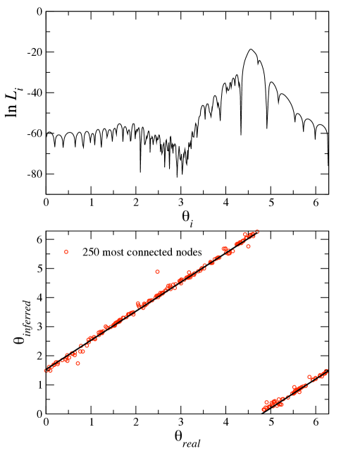
so that $\ln{{\cal L}}=1/2\sum_{i}\ln{{\cal L}_{i}}$. We can interpret function $\ln{{\cal L}_{i}}$ as the fitness of node $i$, which we can then use to maximize the total likelihood. Specifically, in LMH nodes are visited in rounds, and during each round all nodes are visited one by one. At each node visit, the node is moved to the angular position that maximizes its fitness $\ln{{\cal L}_{i}}$, having fixed the positions of all other nodes at that particular node visit. An example of the log-likelihood landscape that a node sees during its move is shown in the top plot of Fig. 7. The total number of rounds of all-node visits needed for LMH to converge is of the order of the network average degree. Indeed, even though after each node move, the fitness of other nodes changes, the node fitness is mostly affected by changes of coordinates of the node neighbors, whose average number thus roughly determines the number of rounds. The maximization of the fitness of a node takes ${\cal O}(N^{2})$ time, having fitness $\ln{{\cal L}_{i}}$ sampled at intervals with $\Delta\theta=1/N$. Therefore for sparse graphs, the overall computational complexity of LMH is ${\cal O}(N^{3})$.

Applied to the real Internet and synthetic Internet-like networks below, both SMH and LMH yield similar good results. However, we prefer LMH since by its localized nature, it can be implemented in a distributed manner, an important property for deployment in the real Internet. Even more importantly, with LMH, new-coming ASs can compute their coordinates in a distributed manner without knowing the global Internet topology. Indeed, to compute its coordinates using Eq. (25), a new-coming AS $i$ has to know the status of connections only to its neighbors; the status of connections between any two ASs other than $i$ does not contribute to $\ln{{\cal L}_{i}}$ in Eq. (25). All results shown in this paper are for LMH.

Figure 7: Top: example of the local log-likelihood of node $i$ (Eq. (25)), having the coordinates of all other nodes fixed at an intermediate step of the mapping process. Bottom: inferred angular coordinates vs. real ones for the 250 most connected nodes in a synthetic $\mathbb{S}^{1}$ network with the same properties as the real Internet: $\gamma=2.1$, $\beta=2$, $N\approx 24000$, $\bar{k}\approx 5$. The LMH kernel and Alg. 1 are used for coordinate inference.

B.3.2 First MLE wrapper

If we naïvly applied any MLE kernel to the Internet, we would have to wait forever for good results. We see in the top plot of Fig. 7 that the characteristic likelihood profile has abundant local maxima. Therefore an MLE kernel is not guaranteed to converge to the global maximum in a reasonable amount of time. It is thus imperative to find a heuristic procedure, i.e., an MLE wrapper, helping an MLE kernel to find its way towards the global maximum without being trapped in local maxima. This procedure is equivalent to using all available information to make an educated guess of the initial node coordinates.

Our MLE wrapping strategy is based on statistical independence of edges in our graphs. Thanks to this independence, the coordinates of a set of nodes can be inferred based only on the partial information contained in a subgraph formed by the nodes in the set, ignoring the rest of the network. Consider a small subgraph of the whole network, for our purposes made of high degree nodes, and remove all nodes and connections not belonging to this subgraph. Since edges in this subgraph are statistically independent of other edges, we can maximize the likelihood corresponding to the subgraph, and infer the coordinates of the nodes in it based only on this partial information. If the subgraph is small and dense enough, finding the optimal MLE solution is easy. Once this solution is found, we can add more nodes to the network, and use the previously inferred coordinates as the initial configuration for the new MLE problem. However, this method works only if the subgraph forms a single connected component. This property holds for synthetic networks in our model, and for the real Internet Serrano et al. (2008).

Formally, let $k_{1},k_{2},\cdots,k_{m}$, with $k_{1}>k_{2}>\cdots>k_{m}$, be a set of predefined degrees, and let ${\cal G}(k_{l})$, $l=1,\cdots,m$, be the subgraphs formed by all nodes of degrees larger or equal to $k_{l}$, plus all connections among them. We thus have ${\cal G}(k_{1})\subset{\cal G}(k_{2})\subset\cdots\subset{\cal G}(k_{m})$, forming a hierarchy of nested subgraphs. The main idea behind our MLE wrapper is to run the MLE kernel, either SMH or LMH, in iterations, starting with the smallest subgraph, and feeding the coordinates inferred at each iteration to the MLE kernel at the next iteration.

This idea must be implemented with care. First, subgraph ${\cal G}(k_{1})$ is different from other subgraphs. Indeed, in scale-free networks, all nodes of degrees larger than $\sim N^{1/2}$ are connected almost surely. Therefore all such nodes would appear identical to the MLE kernel, which would thus place them all at the same location, something that we have to avoid. To solve this problem, we remove all connections among nodes of degree larger or equal to $k_{1}\sim N^{1/2}$ and start the wrapper algorithm with the ${\cal G}(k_{2})$ iteration. Second, iterating from ${\cal G}(k_{l})$ to ${\cal G}(k_{l+1})$, we still need to specify the initial coordinates of the nodes that belong to ${\cal G}(k_{l+1})$ but not to ${\cal G}(k_{l})~{}$. While the assignment of random coordinates to new nodes is possible, it is much more efficient to try to maximize the likelihood in ${\cal G}(k_{l+1})$ from the very beginning. In other words, we assign to each new node $i\in{\cal G}(k_{l+1})\setminus{\cal G}(k_{l})$ the coordinate maximizing

$$\ln{{\cal L}_{i}\left[{\cal G}(k_{l})\right]}=$$ (26)

$$=\sum_{j\in{\cal G}(k_{l})}a_{ij}\ln{p(\chi_{ij})}+\sum_{j\in{\cal G}(k_{l})}(1-a_{ij})\ln{[1-p(\chi_{ij})]}.$$

We note that node $i$ uses information contained only in ${\cal G}(k_{l})$ to get its initial coordinate. After all new nodes corresponding to a given iteration are introduced and assigned initial coordinates, we apply the MLE kernel to the resulting system. This heuristic MLE wrapping procedure is summarized in Alg. 1.

Algorithm 1 First MLE wrapper

  activate nodes in ${\cal G}(k_{1})$

  assign random angular coordinates to nodes in ${\cal G}(k_{1})$

  remove links among nodes in ${\cal G}(k_{1})$

  for $l=2$ to (# of layers) do

        for $j=1$ to (# of nodes in ${\cal G}(k_{l})$ not active) do

              $i\leftarrow$ label of new node in ${\cal G}(k_{l})$ not active

              if # of connections of $i$ with nodes in ${\cal G}(k_{l-1})\geq 2$ then

                    activate new node $i$

                    assign to node $i$ coordinate $\theta_{i}$ maximizing $\ln{{\cal L}_{i}\left[{\cal G}(k_{l-1})\right]}$

              end if

        end for

        run the MLE kernel on the set of active nodes

  end for

Figure 8: Top left: the same as in the bottom plot of Fig. 7 for nodes of degrees $k\geq 20$. All other plots show the results of adding layers of lower degree nodes using the second MLE wrapper with $k_{l_{critic}}=20$. According to Alg. 2, nodes in newly added layers infer their coordinates using the coordinates of nodes in existing layers, without running the MLE kernel, and the coordinates of existing nodes do not change as new nodes are added.

In the bottom plot in Fig. 7 we show the test results for this procedure wrapping the LMH kernel, applied to a synthetic Newtonian–$\mathbb{S}^{1}$ network generated with the parameters similar to the real AS graph. We observe that the inferred coordinates are very close to the real ones, except for a global phase shift, which can take any value in $[0,2\pi]$ due to the rotational symmetry of the model.

B.3.3 Second MLE wrapper

As mentioned above, it is not necessary to consider the full graph to infer the coordinates of the most connected nodes. We now use this observation to speed up the mapping process significantly. Specifically, we run our first MLE wrapper up to a subgraph of a certain size, and then add the rest of the nodes assigning to them their coordinates maximizing Eq. (26) without subsequent running the MLE kernel, see Alg. 2.

This modification speeds the overall mapping process because once the coordinates of the coordinates of a relative small number of high degree nodes are inferred, the rest of the process takes ${\cal O}(N^{2})$ steps to complete. This improvement reduces the total running time of the Internet mapping to few hours on a standard computer. Another practically important feature of this second MLE wrapper is that new-coming ASs compute their coordinates without existing ASs changing their coordinates. In other words, once the AS coordinates are inferred, they stay static as the Internet grows.

Algorithm 2 Second MLE wrapper

  activate nodes in ${\cal G}(k_{1})$

  assign random angular coordinates to nodes in ${\cal G}(k_{1})$

  remove links among nodes in ${\cal G}(k_{1})$

  $l_{critic}\leftarrow$ maximum layer with full MLE calculations

  for $l=2$ to (# of layers) do

        for $j=1$ to (# of nodes in ${\cal G}(k_{l})$ not active) do

              $i\leftarrow$ label of new node in ${\cal G}(k_{l})$ not active

              if # of connections of $i$ with nodes in ${\cal G}(k_{l-1})\geq 2$ then

                    activate new node $i$

                    assign to node $i$ coordinate $\theta_{i}$ maximizing $\ln{{\cal L}_{i}\left[{\cal G}(k_{l-1})\right]}$

              end if

        end for

        if $l\leq l_{critic}$ then

              run the MLE kernel on the set of active nodes

        end if

  end for

Figure 9: Empirical connection probability based on the inferred node coordinates, compared to the connection probability used to generate the synthetic network. The inset shows the details in the small distance region.

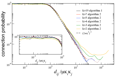
We apply this procedure up to nodes of degree $3$. Nodes of degree $2$ and $1$ must be analyzed separately since all nodes of degree $1$, and $40\%$ of nodes of degree $2$ do not form any triangles. As a consequence, the MLE kernel cannot reliably infer their metric attributes, i.e., their coordinates. Therefore we assign to these nodes the angular coordinate of their (highest-degree) neighbors, which makes sense, especially for nodes of degree $1$, since the only path to such nodes is via their neighbors. Forwarding to such nodes is thus equivalent to forwarding to their neighbors.

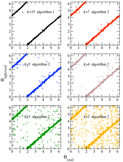
The test results of this second MLE wrapper are shown in Fig. 8. The top left plot shows the inferred vs. real coordinates in the same synthetic network for nodes with degrees $k\geq 20$ using the first MLE wrapper. The other plots show the corresponding coordinates for nodes with degrees larger than or equal to $8,6,5,4,3$ using the second MLE wrapper with $k_{l_{critic}}=20$. That is, the MLE kernel is not run for these nodes. We observe that the inference quality does deteriorate for smaller degrees, but it is remarkable that even in the worst case a majority of coordinates are correctly inferred.

As an additional test, we show in Fig. 9 the empirical connection probability among nodes in each subgraph using the coordinates inferred by the second MLE wrapper, compared to the connection probability $p(x)=(1+x^{2})^{-1}$ used to generate the network. We observe a good agreement for high degree subgraphs, which slightly deteriorates for low degree nodes located at large effective distances $\chi$.

To map the AS graph, we used the LMH kernel wrapped with the second MLE wrapper with $k_{l_{critic}}=20$ and the subgraph hierarchy defined by $k_{1}=300$, $k_{2}=200$, $k_{3}=160$, $k_{4}=130$, $k_{5}=110$, $k_{6}=100$, $k_{7}=90$, $k_{8}=80$, $k_{9}=70$, $k_{10}=60$, $k_{11}=50$, $k_{12}=40$, $k_{13}=30$, $k_{14}=20$, $k_{15}=10$, $k_{16}=9$, $k_{17}=8$, $k_{18}=7$, $k_{19}=6$, $k_{20}=5$, $k_{21}=4$, $k_{22}=3$.

B.4 Parameter estimation and finite size effect

Our model has three parameters: the exponent $\gamma$ of the degree distribution, the average degree $\bar{k}$, and the exponent $\beta$ of the connection probability.

B.4.1 Estimating $\gamma$

We estimate the exponent $\gamma$ via the direct inspection of the degree distribution, yielding $\gamma=2.1$.

B.4.2 Estimating $N$ and $\bar{k}$

The estimation of $N$ and $\bar{k}$ is more involved for two reasons. First, the Newtonian–$\mathbb{S}^{1}$ model generates nodes of zero degree which are included in the computation of the average degree, $\bar{k}=\sum_{k=0}kP(k)$. However, in the real Internet graph all nodes have non-zero degrees. Therefore we first have to estimate the number of nodes $N$ in the model, based on the number of nodes $N_{obs}$ we observe in the real graph. The relationship between the two numbers is

$$N=\frac{N_{obs}}{1-P(0)},$$ (27)

where $P(0)$ is the probability that a node has zero degree in the model.

The second complication is due to finite size effects. These effects are particularly important when the exponent $\gamma$ is close to $2$, which is the case with the Internet. Suppose we generate a finite size network of $N$ nodes with our Newtonian–$\mathbb{S}^{1}$ model with parameters $\gamma$, $\bar{k}$, and $\beta$. Since the network is finite, there is a cut-off value for the expected degree of a node, $\kappa_{c}$, which depends on the size of the network. The first moment of the distribution of expected degrees $\rho(\kappa)=\kappa_{0}^{\gamma-1}(\gamma-1)\kappa^{-\gamma}$ with this cut-off is

$$\langle\kappa(N)\rangle=\bar{k}\left(1-\left[\frac{\kappa_{0}}{\kappa_{c}}\right]^{\gamma-2}\right)\equiv\bar{k}\alpha(\kappa_{0},\kappa_{c}).$$ (28)

In the thermodynamic limit $\kappa_{c}\rightarrow\infty$ and $\alpha(\kappa_{0},\kappa_{c})\rightarrow 1$. However, if $\gamma$ is close to $2$, the approach to these limits is slow, and we have to take care of finite size corrections.

Accounting for these corrections, the expected degree of a node with hidden variable $\kappa$ becomes

$$\bar{k}_{N}(\kappa)=\alpha(\kappa_{0},\kappa_{c})\kappa,$$ (29)

with $\bar{k}_{\infty}(\kappa)=\kappa$. This equation implies that the MLE of the hidden variable $\kappa$ of a node of degree $k$ changes from Eq. (23) to

$$\kappa^{*}=\max{\left(\frac{\gamma-2}{\gamma-1}\bar{k},\frac{1}{\alpha(\kappa_{0},\kappa_{c})}\left[k-\frac{\gamma}{\beta}\right]\right)},$$ (30)

while the average degree including zero degree nodes in a finite size network becomes

$$\bar{k}_{N}=[\alpha(\kappa_{0},\kappa_{c})]^{2}\bar{k}.$$ (31)

If the average degree observed in the real Internet graph is $\bar{k}_{obs}$, our estimate of the parameter $\bar{k}$ is then

$$\bar{k}=\frac{1-P(0)}{[\alpha(\kappa_{0},\kappa_{c})]^{2}}\bar{k}_{obs}.$$ (32)

Therefore, in order to estimate the values of $N$ and $\bar{k}$ for a finite network, we first have to estimate the values of $P(0)$ and $\alpha(\kappa_{0},\kappa_{c})$. One can check Serrano et al. (2008) that

$$P(0)=(\gamma-1)[\alpha(\kappa_{0},\kappa_{c})\kappa_{0}]^{\gamma-1}\Gamma(1-\gamma,\alpha(\kappa_{0},\kappa_{c})\kappa_{0}),$$ (33)

where $\Gamma(x,y)$ is the incomplete Gamma function. We can also relate the maximum degree $k^{\max}_{obs}$ observed in the real Internet to the expected degree cut-off $\kappa_{c}$ via

$$k^{\max}_{obs}=\alpha(\kappa_{0},\kappa_{c})\kappa_{c}.$$ (34)

We thus have six unknown values—namely, $N$, $P(0)$, $\kappa_{0}$, $\kappa_{c}$, $\alpha(\kappa_{0},\kappa_{c})$, and $\bar{k}$—and the system of six equations (9,27,28,32,33,34) involving them. Substituting into these equations the given values of $N_{obs}=23752$, $\bar{k}_{obs}=4.92$, $k^{\max}_{obs}=2778$, and $\gamma=2.1$ observed in the Internet, we compute numerically $\kappa_{0}=0.9$, $\kappa_{c}=4790$, $\alpha(\kappa_{0},\kappa_{c})=0.58$, and $P(0)=0.33$, yielding $N=35685$ and $\bar{k}=9.86$.

B.4.3 Estimating $\beta$

Figure 10: Success ratio of greedy forwarding as a function of $\beta$ for the Internet graph mapping.

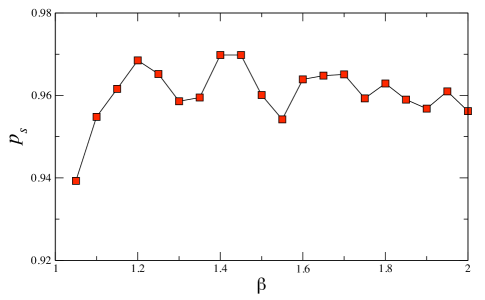
To estimate $\beta$, we first compare clustering in synthetic networks with different $\beta$’s to the clustering observed in the Internet, keeping all other parameters fixed. This procedure narrows down the possible values of $\beta$ to $\beta\in[1,2]$. We then generate Internet maps for different values of $\beta$ within this range, and perform hyperbolic greedy forwarding in them. Fig. 10 shows the success ratio of greedy forwarding as a function of $\beta$ in this region. We observe that the success ratio increases as $\beta$ decreases, and then sharply drops at $\beta\sim 1$. The value of $\beta$ maximizing the success ratio is $\beta=1.45$, and we used this value in our final Internet map.

Appendix C The Archipelago Internet topology

We use the AS Internet topology of June 2009 extracted from the data collected by the Archipelago active measurement infrastructure (ARK) developed by CAIDA Claffy et al. (2009). The AS topology contains $23752$ ASs and $58416$ AS links, yielding the average AS degree $\bar{k}=4.92$. The maximum AS degree is $k^{\max}=2778$. The average clustering measured over ASs of degree larger than $1$ is $\bar{C}=0.61$, yielding temperature $T=0.69$, and hyperbolic disc radius $R=27$. The exponent of the power-law AS degree distribution is $\gamma=2.1$. This Internet topology, along with the hyperbolic Internet map, are released with this paper BoP .

Appendix D Mapping AS’s to countries

The AS-to-country mapping is taken from the CAIDA AS ranking project Dimitropoulos et al. (2007). It uses two methods for this task. The first method is IP-based. It splits the IP address space advertised by an AS into small blocks, and then maps each block to a country using Digital Envoy . If not all IP blocks of an AS map to the same country, then the other, WHOIS-based method is used, which reports the country where the AS headquarters are located according to the WHOIS database WHOIS database . Since large ASs have points of presence in many countries, they tend to map to multiple countries using the IP-based method. Therefore, if we did not apply the WHOIS-based method to them, they would no longer map to a single country. If we ignored such ASs, the angular distributions of the remaining ASs belonging to a given country would be even more localised, including the US, EU, and UK ASs. In our hyperbolic map data, we release the AS-to-country associations using both methods, IP+WHOIS-based and IP-based. The latter has no country information for many ASs with conflicting country mappings.

Appendix E Geographic routing

To perform standard geographic routing we first map each AS to a collection of geographic locations (characterised by their latitudes and longitudes) using the IP-based method, and then find the centre of mass for each collection. We thus obtain unique geographic coordinates for each AS. We then perform standard greedy forwarding over the AS topology, computing geographic distances between ASs using the spherical law of cosines. For hyperbolised geographic routing, we keep the AS angular coordinates equal to their geographic coordinates, but also, based on the AS degree, we assign to each AS a radial coordinate, according to the relationship between node degrees and radial positions in the three-dimensional Einsteinian model, and then perform greedy forwarding in this three-dimensional hyperbolic space.

Appendix F Traffic and congestion considerations

Figure 11: Top: standard normalized betweenness as a function of the AS degree for shortest path forwarding and greedy forwarding. The solid line is a power law of exponent $1.2$. Bottom: normalized betweenness divided by number of routers in the AS, with source and destination ASs chosen with a probability proportional to the number of routers in them.

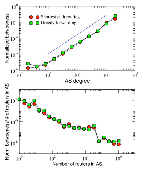
In this section we measure a proxy for the amount of traffic that ASs would have to handle under greedy forwarding.

In view of our finding that greedy forwarding follows almost always the shortest paths, we expect that the traffic load on an AS under greedy forwarding is essentially the same as under shortest path forwarding. We confirm this expectation in Fig. 11 where we juxtapose the normalized betweennesses corresponding to shortest path and greedy forwarding. To compute normalized betweenness, we select a large number of source/destination AS pairs chosen uniformly at random among all ASs. We then find two paths for each AS pair using shortest path and greedy forwarding. Normalized betweenness of a given AS is then the fraction of all paths going through this AS. We observe in Fig. 11 that the normalized betweennesses for shortest path and greedy forwarding are almost identical as expected. We also observe in the top plot, that in agreement with the previous studies on this subject, e.g. Barthélemy (2004), the normalized betweenness grows as a power law of the AS degree. This observation may create an impression that high-degree ASs may suffer from traffic congestion problems. However, this impression is wrong not only because of the results in Gkantsidis et al. (2003), but also because of the following considerations.

In the real Internet, ASs are not singular nodes but differently sized networks composed of (many) routers. The size of an AS, measured by the number of routers in it, is roughly proportional to the AS degree Tangmunarunkit et al. (2001); Huffaker et al. (2010). ASs of different size generate and consume different volumes of traffic. Also, a larger AS can handle larger transit traffic volumes without being congested. These two observations suggest the following modifications to the top plot in Fig. 11. First, we model traffic with the more realistic assumption that the amount of traffic an AS generates or consumes is proportional to the AS size. That is, instead of choosing source and destination AS pairs at random, we chose each AS with a probability proportional to the number of routers in the AS using the data from Huffaker et al. (2010). Second, we divide the normalized betweenness value for each AS by the number of routers in the AS, thus estimating the per-router traffic load. The result shown in the bottom plot of Fig. 11 demonstrates that the important large ASs are, in fact, less prone to congestion problems.

Appendix G Dealing with new-coming AS’s

In this section we show that if the existing ASs keep their hyperbolic coordinates fixed, while the ASs joining the Internet anew over years compute their coordinates in a localizing manner, i.e., using the LMH kernel (25), then the performance of greedy forwarding does not significantly degrade, even at long time scales.

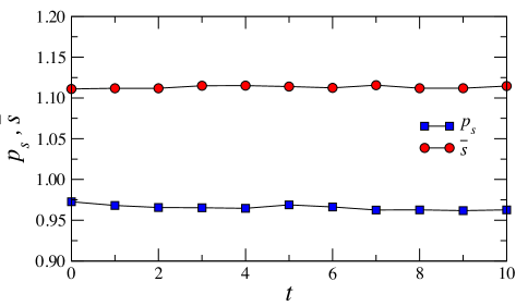
To demonstrate this we perform the following experiment. We replay the AS Internet growth from January 2007 to June 2009 similar to Dhamdhere and Dovrolis (2008). Specifically, we obtain $11$ lists of ASs observed in the Internet at different dates as described in Dhamdhere and Dovrolis (2008). The AS lists are linearly spaced in time with the interval of three months: time $t=0$ corresponds to January 2007, $t=1$ is April 2007, and so on until $t=10$, June 2009. We denote the obtained AS lists by $A_{t}$. The number of ASs in $A_{0}$ is $17258$, while the numbers of new ASs in $A_{t^{\prime}}$ with $t^{\prime}=1,2,\ldots,10$, but not in $A_{0}$ are $806$, $1614$, $2389$, $3103$, $3973$, $4794$, $5434$, $5843$, $6207$, and $6426$. We then take our Archipelago AS topology Claffy et al. (2009) of June 2009, and for each $t=0,1,\ldots,10$ we remove from it all ASs and their adjacent links that are not in $A_{t}$, thus obtaining a time series of historical AS topologies $G_{t}$. We then embed $G_{0}$ using the SMH kernel (24), but for each subsequent embedding of $G_{t^{\prime}}$ with $t^{\prime}>0$, we keep the hyperbolic coordinates of ASs in $G_{t}$ with $t<t^{\prime}$ fixed, and compute coordinates for the new ASs using the LMH kernel (25). That is, once an AS appears at some time $t\geqslant 0$ and gets its coordinates computed, using either the SMH, $t=0$, or LMH, $t>0$, computations, the AS then never changes its coordinates for the rest of the observation period. In Fig. 12 we show the average success ratio $p_{s}$ and stretch $\bar{s}$ for greedy forwarding in $G_{t}$.

Remarkably, we observe only minor variations of success ratio and stretch over more than $2.5$ years of rapid Internet growth. The success ratio does decrease, but by less than $1\%$. We thus conclude that greedy forwarding using our hyperbolic AS map is quite robust with respect to Internet historical growth. Existing ASs do not have to recompute their hyperbolic coordinates when new ASs join the Internet. Recomputations of all AS coordinates may be executed to improve the greedy forwarding performance, but the time scale for such recomputations exceeds the time scale of Internet historical evolution, i.e., years, thus exceeding by orders of magnitude the time scale of transient dynamics of failing AS links and nodes, i.e., seconds or minutes. That is why the existing AS coordinates are essentially static, and can stay the same for years.

Figure 12: Average success ratio $p_{s}$ and stretch $\bar{s}$ for greedy forwarding in the AS Internet growing from January 2007 ($t=0$) to June 2009 ($t=10$) with linear time steps ($\Delta t=1$) of three months, e.g., $t=1$ corresponds to April 2007.

Appendix H Sensitivity to missing links

It is widely known that the existing measurements of the Internet topology miss a number of AS links Lakhina et al. (2003); Dimitropoulos et al. (2007); Oliveira et al. (2010). However, in view of the robustness of greedy forwarding performance with respect to link removals, one could expect that its performance would be robust with respect to missing links as well. Furthermore, if our hyperbolic map is used in practice, then greedy forwarding will see and use those links that we do not see. Therefore one can intuitively expect that, in this case, the efficiency of greedy forwarding will be actually higher than we report in this paper, simply because these links that we miss but greedy forwarding would not miss, would provide additional shortcuts between potentially remote ASs. If so, the routing results presented in this paper should be considered as lower bounds.

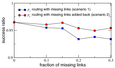
To confirm this intuition, we perform the following experiment. It is known that the majority of missing links in the Internet are peer-to-peer links among provider ASs of moderate size Dimitropoulos et al. (2007); Oliveira et al. (2010). To emulate the missing link issue, we thus remove a fraction (ranging from $0\%$ to $30\%$) of links among nodes with degree above a certain threshold ($k=5$) from our AS graph. We then map these graphs with different numbers of emulated missing links to $\mathbb{H}^{2}$ as described in Section B to find hyperbolic coordinates for each AS. Using these maps with missing information, we then consider two different greedy forwarding scenarios for each map:

1. In the first scenario, we navigate an AS graph mapped with a fraction of links removed, and compute the success ratio of greedy forwarding in the graph. This scenario tries to mimic the missing links issue directly. We have incomplete topology measurements of the real Internet, but we have no other option as to use these measurements to map the Internet to its hyperbolic space, and study navigability with this map, which we know miss some information.

2. In the second scenario, we use the hyperbolic map obtained with missing links, but we then add back those removed links, and navigate the complete graph. This scenario is motivated by the observation that even though our map is constructed with some links missing, these missing links will still be used by ASs attached to them to forward information if this map is used in practice.

The results of these two scenarios are shown in Fig. 13. As intuitively expected, our mapping is quite robust with respect to missing links: the success ratio decreases by less than $5\%$ even if up to $14\%$ of links are removed from the topology before we map it. Also as expected, the missing links, when added back, increase the success ratio. That is, even though the map has been constructed using partial information, navigability improves when missing links are considered. These results confirm that the routing results reported in this paper are in reality lower bounds for the success ratio that can be achieved if our map is used in practice. In fact, one may somewhat paradoxically expect that the more links are missed in the measured Internet topology we used for mapping, the better the success ratio would be in practice, since according to Fig. 13, the success ratio improvement due to re-adding of removed links tends to increase with the number of removed links.

Figure 13: Success ratio as a function of the fraction of removed links among nodes of degree above $5$ for the two scenarios described in the text. Note that $30\%$ of missing links in this subgraph corresponds to $14\%$ of the total number of links in the network.

Appendix I Comments on AS-level routing

Our approach belongs to a wide class of approaches proposing to reduce routing granularity to the level of Autonomous Systems Castineyra et al. (1996); Hinden (1996); Kastenholz (2002); Verkaik et al. (2004); Gummadi et al. (2004); Subramanian et al. (2005); Caesar et al. (2006); Krioukov et al. (2007); Oliveira et al. (2007); Massey et al. (2007); Zhang et al. (2009); Farinacci et al. (2009); Shue and Gupta (2010). The key difference between ours and the existing approaches in this class is that the latter require some form of routing on the dynamic AS graph. As soon as the AS topology changes, new AS routes must be recomputed, so that routing communication overhead is unavoidable in this case. In our case such recomputations are not needed since as we have shown, the efficiency of greedy forwarding sustains in presence of failing AS nodes and links, even though ASs do not exchange any information about topology modifications, and do not change their hyperbolic coordinates, i.e., even though they do not incur any communication overhead. A bulk of routing overhead in the Internet today is due to traffic engineering and multihoming in the first place Huston (2001, 2006). How the AS-level routing class of approaches helps to deal with and reduce this overhead is discussed in the literature cited above.