A Simple Redistribution Vortex Method (with Accurate Body Forces)

Abstract

A circulation redistribution scheme for viscous flow is presented. Unlike other redistribution methods, it operates by transferring the circulation to a set of fixed nodes rather than neighbouring vortex elements. A new distribution of vortex elements can then be constructed from the circulation on the nodes. The solution to the redistribution problem can be written explicitly as a set of algebraic formulae, producing a method which is simple and efficient. The scheme works with the circulation contained in the vortex elements only, and does not require overlap of vortex cores. With a body fitted redistribution mesh, smooth and accurate estimates of the pointwise surface forces can be obtained. The ability of the scheme to produce high resolution solution is demonstrated using a series of test problems.

Keywords: Discrete Vortex Method, particle methods, Lagrangian methods, viscous flow

1 Introduction

Discrete Vortex Methods (DVM’s) are Lagrangian methods for solving for rotational fluid flow in which the vorticity field is partitioned into a finite number of discrete vortex elements, and the evolution of the flow field is determined by following the motion of the vortex elements. One advantage of DVM’s is that the computational effort is applied only in the regions of most interest. Also, for flow past bodies, the far field conditions are automatically satisfied as the vorticity field will decay to zero away from the body, avoiding the problems that can occur when truncating the domain in grid based methods.

For two-dimensional inviscid flow, there is a single component of vorticity, and for inviscid flow, the elements are convected with constant strength at the local velocity of the fluid. For viscous flow, some method of modelling the viscous diffusion must to added to the numerical scheme. A number of schemes have been developed. One of the first applications of a DVM for viscous flow [1] used a random walk to model the viscous effects. A random walk is simple to apply but has relatively low resolution and produces noisy results. A more sophisticated method is the Particle Strength Exchange (PSE) method, introduced in [2], which models the viscous effects using integral operators. A related method is the vorticity redistribution method of Shankar and van Dommelen [3, 4] which, like PSE, involves redistributing circulation between the elements, but does not require a regular mesh, introducing elements locally as required. A more recent redistribution. based on time dependent Gaussian cores, is given by [5]. A description of many aspects of vortex methods can be found in the book by Cottet and Koumoutsakos [6]. Also, a comparison of four viscous methods which do not require the introduction of a grid can be found in [7].

Many papers on vortex use the total force (coefficients) to assess the accuracy of the method but do not present details of the pointwise surface forces. These are frequently noisy due to the irregular distribution of vortex particles, as can be seen in [8], who use random walk for the diffusion. In fact, the total force can also be noisy and require smoothing, as in [8, 9]. In one of the benchmark papers using vortex methods, Koumoutsakos and Leonard [10] do present plots of the surface pressure and vorticity, although they observe high frequency oscillations in the surface vorticity.

Koumoutsakos and Leonard [10] use the PSE method for diffusion. PSE involves the introduction of a grid to the scheme with frequent remeshing in order to maintain the accuracy of the calculation. It appears that the order introduced into the method by the remeshing helps smooth out the spurious high frequency oscillation in the forces that are found in some other methods. Hence, a possible way of reducing the noise would be to remesh every time step with a PSE method. However, an alternative is to combine the remeshing and diffusion operation in single step. This can be done by making the redistribution of the circulation satisfy certain constraints which have a physical meaning. This is a variation of the redistribution method of Shankar and van Dommelen [3], but rather than redistributing circulation between vortex elements, the circulation contained in each discrete vortex element is independently transferred onto a small set of neighbouring nodes . The solution for this redistribution problem can be written explicitly as a set of algebraic equations. The result is a simple, efficient scheme which maintains a regular distribution of vortex elements. The surface force can be calculated directly from local variables, showing very good agreement with test data. Also, since this scheme works with the circulation of a vortex element, independent of the vorticity distribution in the element, there is no requirement for overlap of cores, as in the PSE method.

The paper is structured as follows; first, an outline of the basic method is presented. This is followed by a description of the redistribution scheme. Means of calculating the body forces are then discussed. A brief description of the finite-spectral code used to generate test data is given. Test results are then presented for impulsively started flow past a cylinder and a square. Finally, some conclusions are given.

2 Basic Method

The two-dimensional incompressible Navier-Stokes equation in vorticity form is

$${D\omega\over Dt}~{}=~{}{\partial\omega\over\partial t}\,+\,u\,{\partial\omega\over\partial x}\,+\,v\,{\partial\omega\over\partial y}~{}=~{}\frac{1}{Re}\nabla^{2}\omega$$ (1)

where $(u,v)$ are the velocity components in Cartesian coordinates $(x,y)$, $t$ is the time, $\omega$ the vorticity, $Re$ the Reynolds number, and $\nabla^{2}$ the two-dimensional Laplace operator. The velocity is normalised by the free stream velocity $U_{0}$, the length scales by a characteristic length $L$, and time by $L/U_{0}$. The Reynolds number is given by $\rho LU_{0}/\mu$ with $\rho$ and fluid density and $\mu$ its dynamic viscosity.

Consider an individual vortex element centred on $z=z_{j}$ where $z=x+i\,y$ gives the coordinates in complex form, with a vorticity distribution $\gamma(\eta)$ where $\eta=|z-z_{j}|$, where $2\pi\int_{0}^{\infty}\gamma(\eta)\eta\,d\eta=1$ so that the distribution function has unit circulation. The vorticity field is represented by $N$ discrete vortex elements so that

$$\omega~{}=~{}\sum_{j=1}^{N}\,\Gamma_{j}\,\gamma(|z-z_{j}|)$$ (2)

where $\Gamma_{j}$ is the strength of vortex $j$.

The velocity generated by the vortex elements is given by

$$u_{b}+i\,v_{b}~{}=~{}\sum_{j=1}^{N}\,i\,\Gamma_{j}{z-z_{j}\over|z-z_{j}|^{2}}F(|z-z_{j}|)$$ (3)

where

$$F(\eta)~{}=~{}\int_{0}^{\eta}\gamma(s)\,s\,ds$$ (4)

A number of different functions can be used for the vorticity distribution $\gamma$. In general, point vortices given by a delta function are not used. Instead, a smooth distribution which does not have the numerical problems associated with point vortices is adopted. A standard distribution, used here, is the Gaussian vortex,

$$\gamma(\eta)~{}=~{}\frac{1}{\pi\sigma^{2}}\,e^{-\eta^{2}/\sigma^{2}}$$ (5)

where $\sigma$ is a measure of the core size of a vortex. This gives

$$F(\eta)~{}=~{}\frac{1}{2\pi}\left[1-e^{-\eta^{2}/\sigma^{2}}\right]$$ (6)

As usual, the boundary conditions at the surface of the body are satisfied by the use of a vortex panel method. Both standard straight, constant strength, vortex panels and the higher order panels given in [9] were investigated. The latter method uses overlapping curved panels with a linear distribution of vorticity along the panels. This allows an accurate representation of a smooth body and produces a velocity distribution which is singularity free. However, there was little difference in the results for the different panels for flow past a circular cylinder if enough panels were used. The cylinder results (Section 8) presented below use the high order panels, but, because of the sharp corners, constant strength, straight panels were used for flow past a square (Section 9).

The velocity now consists of three components,

$${\mathbf{u}}={\mathbf{U}}_{f}+{\mathbf{u}}_{b}+{\mathbf{u}}_{p}$$ (7)

where ${\mathbf{u}}=u+i\,v$ is the fluid velocity, ${\mathbf{U}}_{f}=U_{0}$ is the free stream velocity, ${\mathbf{u}}_{b}=u_{b}+i\,v_{b}$ is the velocity generated by the vortex elements, and ${\mathbf{u}}_{p}=u_{p}+i\,v_{p}$ generated by the panels used to satisfy the boundary conditions at the surface of the body.

Numerically, an operator splitting method is used, with inviscid and viscous sub steps, satisfying

$${D\omega\over Dt}=0$$ (8)

and

$${\partial\omega\over\partial t}=\frac{1}{Re}\nabla^{2}\omega$$ (9)

respectively.

The equation for the inviscid sub step represents the fact that for two-dimensional inviscid flow vorticity is convected by the flow. Numerically, the element vortices are moved at the local fluid velocity, i.e.

$${d{\mathbf{z}}_{j}\over dt}~{}=~{}{\mathbf{u}}({\mathbf{x}}_{j},t)$$ (10)

A second order Runge-Kutta method is used to move the vortices at each time step

$$\hat{\mathbf{z}}_{j}~{}=~{}{\mathbf{z}}^{n}_{j}~{}+~{}\frac{1}{2}\Delta t\,{\mathbf{u}}({\mathbf{z}}_{j},t_{n})$$ (11)

$${\mathbf{z}}^{n+1}_{j}~{}=~{}{\mathbf{z}}^{n}_{j}~{}+~{}\Delta t\,{\mathbf{u}}(\hat{\mathbf{z}}_{j},t_{n+1/2})$$ (12)

A number of methods exist for the viscous sub step (9). The method developed here is based on the vorticity redistribution scheme of Shankar and van Dommelen [3]. In this method, at each time the circulation of vortex elements are updated through

$$\Gamma_{j}^{n+1}=\sum_{k}\Gamma_{k}^{n}W^{n}_{kj}$$ (13)

where $W^{n}_{kj}$ represents the fraction of the circulation of vortex $k$ transferred to vortex $j$ by diffusion during time step $n$. The summation is over a group of vortices local to $z_{j}$, the position of vortex $j$. The fractions $W^{n}_{kj}$ are calculated to satisfy the following constraints

$$\sum_{k}\,W^{n}_{kj}~{}=~{}1$$ (14)

$$\sum_{k}\,W^{n}_{kj}(x_{j}-x_{k})~{}=~{}\sum_{k}\,W^{n}_{kj}(y_{j}-y_{k})~{}=~{}0$$ (15)

$$\sum_{k}\,W^{n}_{kj}(x_{j}-x_{k})^{2}~{}=~{}\sum_{k}\,W^{n}_{kj}(y_{j}-y_{k})^{2}~{}=~{}2\,h_{v}^{2}$$ (16)

$$\sum_{k}\,W^{n}_{kj}(x_{j}-x_{k})(y_{j}-y_{k})~{}=~{}0$$ (17)

where $h_{v}=\surd\overline{\Delta t/Re}$ is the characteristic diffusion distance over time $\Delta t$. Stability requires $W^{n}_{kj}>0$. Equations (14-17) enforce conservation of vorticity, the centre of vorticity, and linear and angular momentum.

The redistribution is performed over all vortices within a distance $Rh_{v}$ of vortex $k$, i.e. such that

$$|z_{j}-z_{k}|\,\leq\,R\,h_{v}$$ (18)

The accuracy of the method depends on the value of $R$ and a minimum value of $R=2$ is required for a first or second order solution to exist [3]. $R=\surd\overline{12}$ was used in [3]. A solution may not always exist, for example if there are less than six vortices within the region (18). If no solution is found, new vortices are introduced a distance $\surd\overline{6}h_{v}$ from the centre ($z_{j}$) until a solution exists. Further details of the method and its theoretical basis can be found in [3].

In this scheme, all vortex elements satisfying (18) must be identified. The redistribution problem can then be solved using a linear programming method, for example the revised simplex scheme found in [11].

3 The Circulation Redistribution scheme

3.1 Redistribution in Cartesian coordinates.

The redistribution scheme above (13-17) operates by transferring circulation between vortex elements, introducing new elements as required. However, an alternative is to transfer the circulation onto a set of nodes at known positions. Consider a one-dimensional unsteady diffusion problem, with a uniform grid with grid step $h$. Suppose there is a vortex of strength $\Gamma$ placed at $x=x_{v}$ where $x_{i}\leq x_{v}\leq x_{i+1}$, and $x_{i}=i\,h$. Let

$$\Delta~{}=~{}(x_{v}-x_{i})/h$$ (19)

Then a solution of the redistribution equations is

$$f_{i}~{}=~{}1\,-\,2\left(\frac{h_{v}}{h}\right)^{2}\,-\,\Delta^{2}$$ (20)

$$f_{i-1}~{}=~{}\frac{1}{2}(1\,-\,f_{i}\,-\,\Delta)$$ (21)

$$f_{i+1}~{}=\frac{1}{2}(1\,-\,f_{i}\,+\,\Delta)$$ (22)

where circulation $\Gamma\,f_{k}$ is transferred to the grid point $x=x_{k}$. All other $f_{k}$ are zero. A second solution is given by

$$g_{i+1}~{}=~{}1\,-\,2\left(\frac{h_{v}}{h}\right)^{2}\,-\,\Delta_{1}^{2}$$ (23)

$$g_{i}~{}=~{}\frac{1}{2}(1\,-\,g_{i+1}\,-\,\Delta_{1})$$ (24)

$$g_{i+2}~{}=\frac{1}{2}(1\,-\,g_{i+1}\,+\,\Delta_{1})$$ (25)

with $g_{k}=0$ for the other $g_{k}$, and $\Delta_{1}=(x_{v}-x_{i+1})/h=\Delta-1$.

In principle either of these solutions could be used. However, consider the case when the element is midway between grid points, i.e. $\Delta=\frac{1}{2}$. On physical grounds, the redistribution would be expected to be symmetric, but both of the solutions are asymmetric. A simple way of producing a symmetric solution in this case is to use the average of the two solutions, i.e. $F_{k}=\frac{1}{2}(f_{k}\,+\,g_{k})$, $k=i-1,\dots,i+2$. This gives the same solution as would be obtained by using the four points $i-1$ to $i+2$ and assuming symmetry ($F_{i-1}=F_{i+2}$ and $F_{i}=F_{i+1}$).

More generally, a linear combination of the two basic solutions, (20-22) and (23-25), can be used

$$F_{k}~{}=~{}(1-\Delta)f_{k}~{}+~{}\Delta g_{k},~{}~{}~{}k=i-1,\dots,i+2$$ (26)

This produces a symmetric three point solution if the element is at a grid point, and a symmetric four point solution if the element is midway between grid points, with a smooth change between these two extreme cases. It is the simplest solution which satisfies both the redistribution equations and symmetry.

Some test calculations have been performed for a circular cylinder case using using only three point formula ((20-22) for $x_{k}\leq x_{0}<\frac{1}{2}(x_{k}+x_{k+1})$ and (23-25) for $\frac{1}{2}(x_{k}+x_{k+1})\leq x_{0}<x_{k+1}$), but these produced undesirable short scale variations in the solution when a vortex element moved across a midpoint and the redistribution changed bias. This did not occur when using the combination (26).

Stability requires that the redistribution fractions are positive. The most restrictive case when using (26) is when the element is at a grid point. The condition is then

$$\frac{h_{v}}{h}\,<\,\frac{1}{\surd 2}$$ (27)

As simple test problem is that of one dimensional diffusion starting from a point distribution of vorticity at $x=x_{0}$ at $t=0$. Figure 1 shows the analytic and redistribution solutions for the vorticity for a test case at $t=1.1$ with $x_{0}=1$, $Re=100$ and total circulation of $\surd(Re/\pi)$. The calculation was started from the analytic solution at $t=0.1$. The grid step was $h=1/100$ and the time step was $t=0.005$. Two different grids were used in the calculation. There was an offset between the grids and they were used alternatively at successive time steps. A number of different offsets, ranging from $\Delta=0$ to $\Delta=1$) were tested, and the good agreement with the analytic solution shown in Figure 1 is typical.

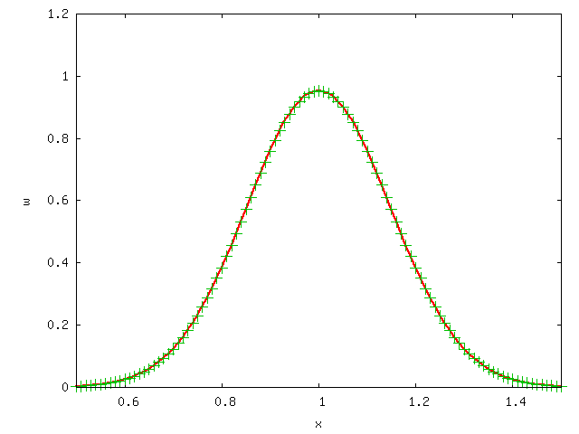
Figure 1: Vorticity distribution for the one dimensional test problem at $t=1.1$ with $Re=100$, $h=1/100$ and $\Delta t=0.005$. The solid line is the analytical solution and the symbols are from the redistribution scheme.

Consider now the two dimensional case in $(x,y)$ with grid $x_{i}=i\,h$ and $y_{j}=j\,\hat{h}$ and a vortex element located at $(x_{v},y_{v})$ where $x_{i}\leq x_{v}<x_{i+1}$ and $y_{j}\leq y_{v}<y_{j+1}$. The one dimensional redistribution in the $y$ direction is given by

$$G_{l}~{}=~{}(1-\delta)\,\hat{f}_{l}~{}+~{}\delta\,\hat{g}_{l},~{}~{}~{}l=j-1,\dots,j+2$$ (28)

where

$$\delta~{}=~{}(y_{v}\,-\,y_{j})/\hat{h}$$ (29)

and the $\hat{f}_{l}$ and $\hat{g}_{l}$ are obtained as in (20-25).

The two dimensional redistribution scheme is given by

$$W_{k,l}~{}=~{}F_{k}\,G_{l},~{}~{}~{}k=i-1,\dots,i+2,~{}~{}l=j-1.\dots,j+2$$ (30)

These weights satisfy all of the constraints in the original redistribution scheme (14-17).

This solution of the redistribution problem satisfies Shankar and van Dommelen condition for the existence of a solution; the simplest two-dimensional solution has a nine point stencil and the stability condition implies that the corner points of the stencil must be a distance of at least $2h_{v}$ from the centre point.

Figure 2 shows typical constant vorticity contours for the two dimensional diffusion problem. Again, two offset grids were used. The contours shown are from the numerical solution. At the scale shown they are identical to the contours from the analytic solution.

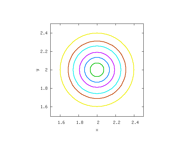
Figure 2: Vorticity distribution for the two dimensional test problem at $t=1.1$ with $Re=100$, $h=\hat{h}=1/100$ and $\Delta t=0.005$. From the centre, the contours are for 0.8, 0.6, 0.4, 0.2, 0.1, and 0.025.

3.2 Redistribution in cylindrical coordinates

The standard case of flow past a circular cylinder will be used as a test for the method. The obvious grid to use in this case is one using polar coordinates $(r,\theta)$. However, the original redistribution equations must be converted to the appropriate form. Transforming between polar and Cartesian coordinates in standard form $x=r\cos\theta$, $y=r\sin\theta$, write

$$x_{k}\,=\,(r_{j}+\Delta r_{k})\cos(\theta_{j}+\Delta\theta_{k}),~{}~{}~{}~{}y_{k}\,=\,(r_{j}+\Delta r_{k})\sin(\theta_{j}+\Delta\theta_{k})$$ (31)

Substituting (31) into (15-17) and expanding, while retaining all terms $O(\Delta^{2}$) or greater, produces the constraints

$$\sum_{k}\,W^{n}_{kj}\,r_{j}\,\Delta r_{k}~{}=~{}h_{v}^{2}$$ (32)

$$\sum_{k}\,W^{n}_{kj}\,r_{j}\,\Delta\theta_{k}~{}=~{}0$$ (33)

$$\sum_{k}\,W^{n}_{kj}\,\Delta r_{k}^{2}~{}=~{}\sum_{k}\,W^{n}_{kj}\,r_{j}^{2}\,\Delta\theta_{k}^{2}~{}=~{}2\,h_{v}^{2}$$ (34)

$$\sum_{k}\,W^{n}_{kj}\,r_{j}\Delta r_{k}\,\Delta\theta_{k}~{}=~{}0$$ (35)

Equations (32-35) are analogous to the original constants (15-17) with the Cartesian lengths replaced by the polar ones ($\Delta r_{k}$ and $r_{v}\Delta\theta_{k}$) apart from the linear radial constraint (32) which has a nonzero right side. This term arises from the $\frac{1}{r}{\partial\over\partial r}$ in the polar Laplace operator; setting the right side of (32) to zero would produce a nonphysical result in which the diffusion operator is ${\partial^{2}\over\partial r^{2}}+\frac{1}{r^{2}}{\partial^{2}\over\partial\theta^{2}}$.

The redistribution formula for the radial one dimensional problem are

$$f_{i}~{}=~{}1\,-\,2\left(\frac{h_{v}}{\Delta r}\right)^{2}\,-\,\Delta^{2}-2\Delta\frac{h_{v}^{2}}{r_{v}\Delta r}$$ (36)

$$f_{i-1}~{}=~{}\frac{1}{2}(1\,-\,f_{i}\,+\,\Delta\,+\,\frac{h_{v}^{2}}{r_{v}\Delta r})$$ (37)

$$f_{i+1}~{}=~{}\frac{1}{2}(1\,-\,f_{i}\,-\,\Delta\,-\,\frac{h_{v}^{2}}{r_{v}\Delta r})$$ (38)

where the radial grid is given by $r_{i}-r_{0}+i\Delta r$, $\Delta=(r_{v}-r_{i})/\Delta R$, and the vortex element is at $r=r_{v}$ where $r_{i}\leq r_{v}<r_{i+1}$.

The second redistribution solution involving the points $i$, $i+1$ and $i+2$ follows in the obvious manner. The azimuthal redistribution solution is obtained from (20-24) with the lengths replaced by $r_{v}\Delta\theta$. Again, linear combinations of the redistribution solutions are formed, and the two dimensional redistribution scheme obtained as in (30).

3.3 Redistribution in general coordinates.

Above the redistribution method has been presented for Cartesian and polar coordinates system. The method extends to other, more general, systems. For example, for a transformation given by $x=f(\eta)$, the condition for first moment in $x$ becomes

$$\sum_{k}\,W^{n}_{kj}\,\Delta\eta_{j}\,f^{\prime}(\eta_{k})~{}=~{}-h_{v}^{2}\frac{f^{\prime\prime}(\eta_{k})}{f^{\prime 2}(\eta_{k})}$$ (39)

where $\Delta\eta_{j}=\eta_{j}-\eta_{k}$ and the other equations are obtained by replacing $x_{j}-x_{k}$ by $\Delta\eta_{j}f^{\prime}(\eta_{k})$. Further, the redistribution problem can formulated for a general grid with fixed nodes by calculating the appropriate terms, a procedure equivalent to calculating the metric terms scaling the derivatives in the diffusion operator in a finite volume method.

4 Computational Algorithm.

The full scheme is a fractional step algorithm consisting of the following steps –

1. Redistribution onto a fixed grid over a time step of $\frac{1}{2}\Delta t$.

2. Convection of the vortex elements using the two-step Runge-Kutta scheme (11,12).

3. Redistribution onto a fixed grid over a time step of $\frac{1}{2}\Delta t$

A method for diffusing vorticity from the surface where it is created must be incorporated into this scheme. A number of methods can be found in the literature. The simplest is to create new vortex elements a small distance off the boundary, as in [12, 9]. In contrast, [10] solve a diffusion problem using the flux of vorticity from the surface as a boundary condition. In [5], the redistribution method is used to diffuse vorticity from the vortex sheet on the boundary into the interior. The last approach is the one used here, in the simplest manner consistent with the algorithm. The circulation from the vortex panels created at the start of step 2 is placed on a set of points on the boundary (the control points used to calculated the strengths of the vortex panels), and these are used as new vortex elements added to the redistribution of step 3. All circulation distributed across the boundary during the redistribution steps is reflected back across the boundary, ensuring conservation of circulation and imposing a no flux boundary condition.

5 Body Forces

The standard way to calculate the lift and drag with a DVM is to use the impulse (see e.g. [13]) -

$$({\cal D,L})\,=\,-{d\over dt}\int(y\omega,-x\omega)dA\,=\,-{d\over dt}\sum_{i}\Gamma_{i}(y_{i},-x_{i})$$ (40)

where $\cal{D}$ and $\cal{L}$ are the drag and lift normalised by $\rho U_{0}^{2}L$ where $L$ is a reference length. The summation is performed over the entire domain $A$ for all circulation carrying elements.

The surface pressure can be related to the strength of the vortex panels [8, 12] through

$$\Delta p~{}=~{}\frac{\Delta\Gamma}{\Delta t}$$ (41)

where $\Delta\Gamma$ is the circulation carried by the relevant portion of the wall.

The wall shear stress is obtained by using a finite difference formula with velocity components evaluated at fixed points near the surface. For the circular cylinder, the redistribution grid has $r_{i}=r_{0}+(i-\frac{1}{2})\Delta r$ where $r_{0}$ is the radius of the cylinder. The shear is calculated using the velocity at midpoints through the one sided, second order formula

$${\partial u_{\theta}\over\partial r}~{}=~{}{-\,3\,u_{\theta}(r_{0})\,+4\,u_{\theta}(r_{0}+\Delta r)\,-\,u_{\theta}(r_{0}+2\Delta r)\over 2\,\Delta r}$$ (42)

where $u_{\theta}$ is the azimuthal velocity.

6 Test Data: Flow Past a Circular Cylinder.

There are a large number of papers which use flow past a circular cylinder as a test case. However, in most of these only the lift and drag (coefficients) are presented. To provide detailed data for comparison, a finite difference-spectral (FDS) code was used. The streamfunction-vorticity formulation is used, with governing equations the vorticity transport equation (1), and the Poisson equation for the streamfunction $\psi$

$$\omega~{}=~{}-\,\nabla^{2}\psi$$ (43)

Fourier modes were used in $\theta$, and second order central difference formula in the radial direction. A one sided backwards difference formula, similar to (42), was used for the time derivative, except for the first time step where a backwards Euler scheme was used. The code is fully implicit, iterating to obtain the solution at each time step. The radial grid was stretched to give a fine grid near the cylinder, and place the outer boundary of the computational domain a long way from the surface. The non-linear terms were handled in the usual pseudo-spectral manner.

With an impulsive start the boundary layer grows as $t^{1/2}$. This scaling was used for the earlier part of the computation, with

$$r\,-\,r_{0}~{}=~{}2\left(\frac{t}{Re}\right)^{\frac{1}{2}}\,\eta,~{}~{}~{}~{}~{}\psi~{}=~{}t^{\frac{1}{2}}\Psi,~{}~{}~{}~{}~{}\omega~{}=~{}t^{-\frac{1}{2}}\,\Omega~{}$$ (44)

The calculation was switched to a fixed grid at $t=1$, using the radial distribution from (44) at this time.

This produces a relatively simple but efficient code in which high accuracy can be obtained by using a large number of Fourier modes and radial grid points and a small time step. Grids of up to 1024 complex Fourier modes, 2000 radial points, and a time step of $10^{-6}$ were used for the data presented below. Grid independence was checked for all Reynolds numbers.

On the surface of the cylinder

$${\partial p\over\partial\theta}~{}=~{}{r_{0}\over Re}\,{\partial\omega\over\partial r}$$ (45)

which can be used to calculate the surface pressure using a reference value of zero at the front of the cylinder. This equation is analogous to (41) for the DVM. Both relate the flux of vorticity from the surface to the pressure gradient.

The results produced by this code compare well with those found in other high resolution simulation (e.g. [10]). Also, they agree with the short time series solutions given by [15, 16].

7 Choice of grid and numerical parameters.

As a test case for the effects of the numerical parameters and grid on the accuracy of the solution, the drag for the flow past an impulsively started cylinder for short time will be used. Lengths are scaled or the diameter of the cylinder $D$ so that the surface of the cylinder is at $r=r_{0}=1/2$, the vorticity is scaled by $U_{0}/D$ where $U_{0}$ is the free stream velocity, and the time is scaled by $D/U_{0}$. The Reynolds number is $Re=U_{0}\,D/\nu$ where $\nu$ is the kinematic viscosity.

A body fitted polar grid is used in the region $r_{0}\leq r\leq r_{1}$. This is embedded in a uniform Cartesian mesh for $r>r_{1}$. The inner grid is arranged so that the surface of the cylinder falls midway between radial grid points, with $r_{i}=r_{0}+(i-\frac{1}{2})\Delta r$ where $\Delta r$ is the radial grid step, so that the surface is at $r=r_{1/2}$. Azimuthally, the grid is placed at uniformly spaced points $\theta=\theta_{j}$ with grid step $\Delta\theta=2\pi/N$ where $N$ is the number of vortex panels. The end of the vortex panels are at $\theta=\theta_{j+1/2}$, with the control points for the evaluation of the boundary velocity at $(r_{0},\theta_{j})$.

The method does not explicitly allow for the $t^{\frac{1}{2}}$ behaviour for small time, so the solution cannot be expected to be accurate over the first few time steps. However, with an appropriate choice of parameters, solutions which achieve high accuracy after a few time steps can be obtained.

There are six numerical parameters which must be chosen. The grid steps in $r$ and $\theta$ for the inner grid, the grid step $h$ for the outer grid (a square grid is used here although this is not required), the region for the inner grid ($r_{1}$), the time step $\Delta t$ and the core size $\sigma$.

The maximum time step is fixed by the stability of the redistribution scheme. Since the algorithm has two redistribution substeps over time $\Delta t/2$, the stability condition becomes $h_{v}/h_{m}<1$, or $\Delta t<Re\,h_{m}^{2}$, where $h_{m}$ is the smallest of the three grid steps $\Delta r$, $r_{0}\Delta\theta$ and $h$.

The effects of the core size were investigated in [9], and they concluded that taking $\sigma=l/4$ where $l$ is the (average) length of a vortex panel was a suitable choice. This works well here also, giving $\sigma=r_{0}\Delta\theta/4$.

The effect of the grid on the solution was investigated by fixing the number of vortex panels and varying $\Delta r$. Figure 3 shows the drag calculated from the impulse (40) for short time for an impulsive start with $Re=550$, 400 panels, $\Delta t=0.025$, and $\Delta r=1/200$, $1/300$ and $1/400$. For the smallest value of $\Delta r$, $h_{v}/\Delta r\approx 0.85$. Apart from the first few steps, the middle value ($\Delta r=1/300$) gives good agreement from the drag for the FDS scheme, while for the smaller value ($\Delta=1/400$) the drag approaches that from the FDS scheme from below. For $\Delta=1/200$, the drag is too large. For clarity, only every fourth point is shown for the solutions for $h=1/300$ and $1/400$. All points are used for $h=1/200$, and no filtering or smoothing has been applied for this figure. The smoothness is typical of the results obtained when using a body fitted redistribution mesh.

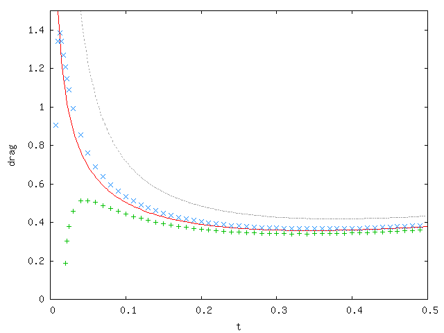
Figure 3: The drag for impulsively started flow past a circular cylinder at $Re=550$ cylinder at $Re=550$ with 400 vortex panels, $r_{1}=\frac{6}{5}$, $\Delta t=0.0025$ and $h=\frac{1}{80}$: dashes, $\Delta r=\frac{1}{200}$; $\times$, $\Delta r=\frac{1}{300}$; $+$, $\Delta r=\frac{1}{400}$. Solid line, FDS solution.

Figure 4 shows the streamwise component of the impulse, $I_{x}=\int y\omega dA$, for the same cases as in Figure 3. For an impulsive start for flow past a cylinder, the initial condition at $t=0^{+}$ is that from potential flow, with a vortex sheet of (nondimensional) strength $\Gamma=-2\sin(\theta)$ on the surface, giving $I_{x}=-\pi/2$. For $t>0$, the impulse should decrease smoothly from the initial value. For $\Delta r=1/300$, there is some (expected) irregular behaviour for the first few time steps, but the impulse is generally well behaved. In contrast, the smaller and larger values of $\Delta r$ produce a jump in the impulse, followed by a relatively fast decrease for $\Delta r=1/200$ and an increase for $\Delta r=1/400$, consistent with the behaviour of the drag (Figure 3).

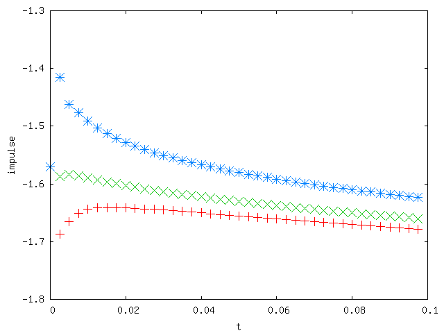
Figure 4: The streamwise component of impulse for impulsively started flow past a circular cylinder at $Re=550$ with 400 vortex panels, $\Delta t=0.0025$ and $h=\frac{1}{80}$: $*$, $\Delta r=\frac{1}{200}$; $\times$, $\Delta r=\frac{1}{300}$; $+$, $\Delta r=\frac{1}{400}$

Calculations were performed for with different time steps (smaller for all three values of $\Delta r$ and larger for $\Delta r=1/200$ and $1/300$), but the behaviour of the impulse was similar to that shown in Figure 4 with an overshoot for $\Delta r=1/200$ and an overshoot for $\Delta r=1/300$. The impulse was examined for a large number of other runs with Reynolds numbers varying from 150 to 9500 and a range of time steps, and its behaviour for short time provides a useful diagnostic as to the quality as the grid with regard to the ratio of the grid steps. This test could be used for other problems in which there is no reliable solution available to compare with, e.g. for flow past a square (Section 9 below).

For all the Reynolds numbers studied, a ratio of approximately 2/5 for the radial to azimuthal grid ($\Delta r/r_{0}\Delta\theta$) with $\sigma=r_{0}\Delta\theta/4$ was found to give an accurate solution provided the time step was small enough. Figure 5 shows the drag for runs with $\Delta t=0.002$, 200 panels and $\Delta r=1/150$, 400 panels and $\Delta r=1/300$, and 600 panels and $\Delta r=1/450$, i.e.  maintaining the same scaling as for 400 panels in Figures 3 and 4. Clearly, the grid is too coarse to provide a good match with the FDS solution very early in the run, but does give a reasonable value for $t>0.1$. As above, there is good match with 400 panels, and a very close match with 600 panels.

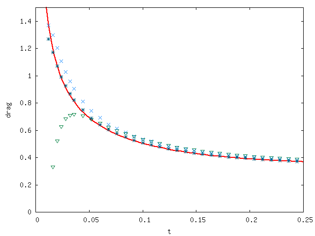
Figure 5: The drag for impulsively started flow past a circular cylinder at $Re=550$ cylinder at $Re=550$ with $\Delta t=0.002$; solid line, FDS solution; $\triangle$, 200 panels; $\times$, 400 panels; $*$, 600 panels.

The outer grid step $h$ and $r_{1}$ were also varied to ensure they did not significantly affect the results shown in Figures 3-5. Tests were also performed with other Reynolds numbers to ensure the results presented below are accurate.

8 DVM solutions: Flow Past a Circular Cylinder.

Calculations were performed for impulsively started flow past a circular cylinder using Reynolds numbers of 150, 550, 1000, 3000, and 9500. These Reynolds numbers were chosen as they are commonly used as test cases. A large of amount of test data was generated, showing excellent agreement with the results from the FDS code in all cases (and with data found in other studies). Representative results are presented for three Reynolds numbers ($Re=150$, 1000, and 9500), covering three orders of magnitude.

8.1 $\mathbf{Re=150}.$

Figure 6 shows the total drag obtained from the DVM and FDS methods for flow with $Re=150$. The numerical parameters are $N=400$, $\Delta r=1/320$, $\Delta t=0.001$ ($h_{v}/\Delta r=0.32$), $r_{1}=1$ and $h=1/100$. For the DVM, both the drag from the impulse (40) and that from the pressure and wall shear stress (41-42) are shown. There is excellent agreement between all methods. Figure 7 shows the pressure and wall shear stress components of the drag obtained from the DVM and FDS schemes. Again there is excellent agreement.

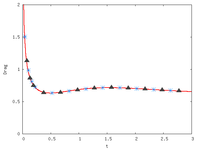
Figure 6: Total drag for impulsively started flow past a circular cylinder at $Re=150$. Line: FDS solution. Symbols: DVM solution, $*$ from the impulse(40), $\triangle$ from the surface forces (41-42).

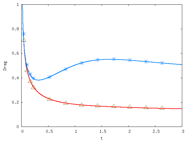
Figure 7: Drag components for impulsively started flow past a circular cylinder at $Re=150$. Upper, pressure component. Lower, shear stress component. Lines: FDS solution. Symbols: DVM solution.

The surface distribution of pressure and wall shear stress at a single point in time ($t=1$) are shown in Figures 8 and 9. There is very good agreement between the values from the two numerical schemes. Figure 10 shows contours of the vorticity at $t=1$, with the upper half of the plot showing the contours from the DVM method and the lower from the FDS scheme. Again, there is excellent agreement.

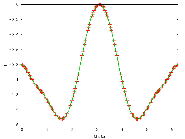
Figure 8: Surface pressure $p$ against $\theta$ at $t=1$ for $Re=150$. $\theta$ is in radians measured from the rear of the cylinder. The reference value is zero at the front of the cylinder ($\theta=\pi$). Symbols: DVM solution, line: finite difference solution.

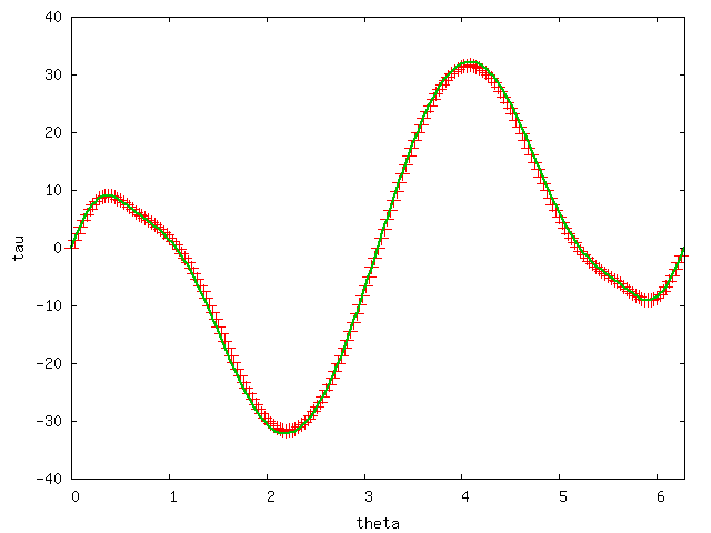
Figure 9: Wall shear stress against $\theta$ at $t=1$ for $Re=150$. Symbols: DVM solution, line: finite difference solution.

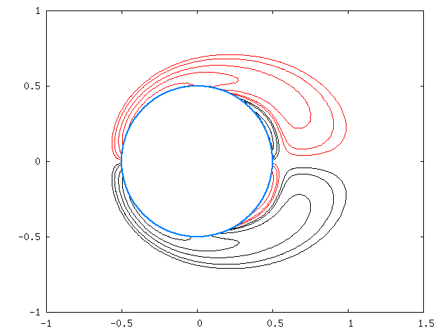
Figure 10: Vorticity contours for $Re=150$ at $t=1$: black, positive; red, negative. Going from the far field towards the cylinder, the contours are for $|\omega|$=1,2,5,10,20. The contours above the axis ($y>0$) are from the DVM code, and those below the axis from the FDS code.

8.2 $\mathbf{Re=1000}.$

Figures 11 and 12 show the total drag and drag components for the two methods for flow with $Re=1000$. The numerical parameters are $N=600$, $\Delta r=1/480$, $\Delta t=0.0025$ ($h_{v}/\Delta r\approx 0.76$), $r_{1}=1$ and $h=1/480$. As for $Re=150$, there is excellent agreement. Also, very good agreement is obtained for the surface forces and contours of vorticity, as can be seen for $t=3$ in Figures 13, 14 and 15.

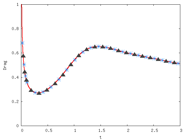
Figure 11: Total drag for impulsively started flow past a circular cylinder at $Re=10^{3}$. Line: FDS solution. Symbols: DVM solution, $*$ from the impulse(40), $\triangle$ from the surface forces (41-42).

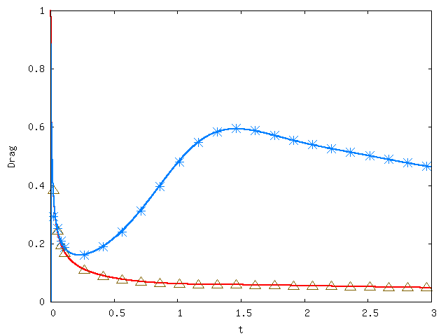
Figure 12: Drag components for impulsively started flow past a circular cylinder at $Re=10^{3}$. Upper, pressure component. Lower, shear stress component. Symbols: DVM solution. Lines: finite difference solution.

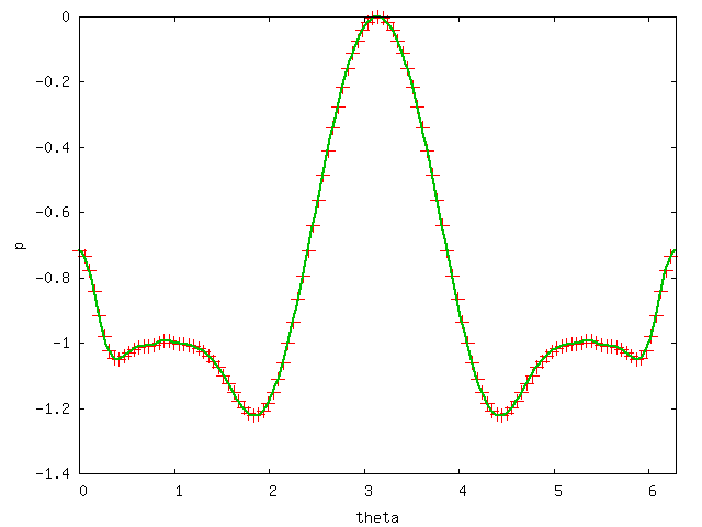
Figure 13: Surface pressure $p$ against $\theta$ at $t=3$ for $Re=10^{3}$. $\theta$ is in radians measured from the rear of the cylinder. The reference value is zero at the front of the cylinder ($\theta=\pi$). Symbols: DVM solution, line: finite difference solution.

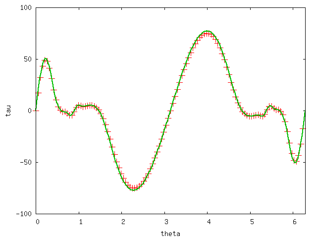
Figure 14: Skin friction against $\theta$ at $t=3$ for $Re=10^{3}$. Symbols: DVM solution, line: finite difference solution.

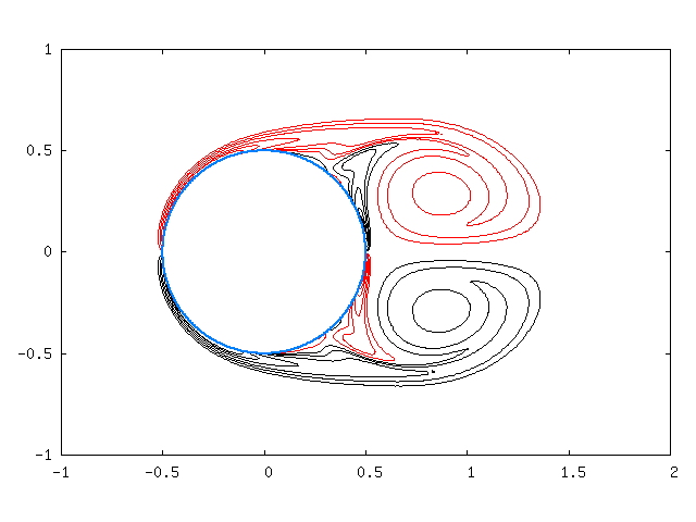
Figure 15: Vorticity contours for $Re=10^{3}$ at $t=3$: black, positive; red, negative. Going from the far field towards the cylinder, the contours are for $|\omega|$=2,5,10,30,40. The contours above the axis ($y>0$) are from the DVM code, and those below the axis from the FDS code.

8.3 $\mathbf{Re=9500}.$

Flow with $Re=9500$ provides a much stiffer test of the method as the flow field is more complex, with short scale variations in the surface forces and a much more complicated vorticity pattern than that found with lower Reynolds numbers. Again, however, there is very good agreement between the solutions for the two numerical schemes.

Figures 16 and 17 show the total drag and drag components. The numerical parameters are $N=3000$, $\Delta r=1/2400$, $\Delta t=0.001$ ($h_{v}/\Delta r\approx 0.78$), $r_{1}=6/5$ and $h=1/800$. The surface forces at $t=2$ are shown in Figures 18, 19. There is a high level of agreement, in particular, in the wall shear stress on the rear part of the cylinder where the development of relatively small scale but strong structures in the flow lead to large peaks and high values of the gradient along the surface. The complex nature of the flow can also be seen in the vorticity contours (Figure 20).

The values of the wall shear stress at the top and bottom shoulder of the cylinder ($\theta=\pi/2$ and $3\pi/2$) are slightly lower for the DVM method as compared with those for from the FDS calculations. However, the radial grid used for the DVM calculation near the surface is coarse as compared to that for FDS, and it was found that increasing the resolution gave a better match, but with an increase in computational effort.

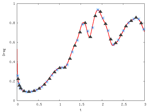
Figure 16: Total drag for impulsively started flow past a circular cylinder at $Re=9500$. Line: FDS solution. Symbols: DVM solution, $*$ from the impulse(40), $\triangle$ from the surface forces (41-42).

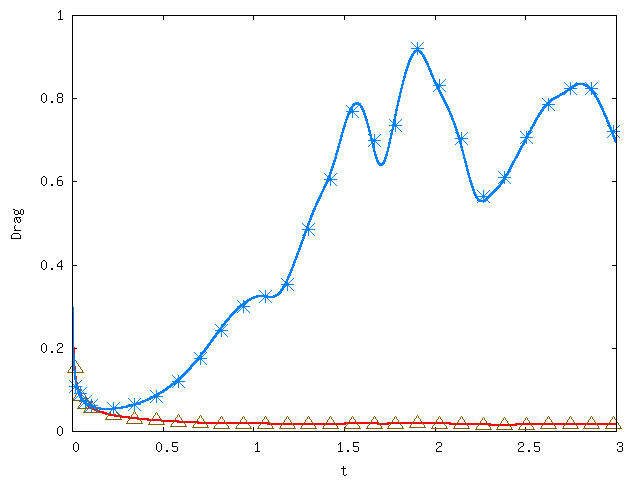
Figure 17: Drag components for impulsively started flow past a circular cylinder at $Re=9500$. Symbols: DVM solution. Lines: finite difference solution.

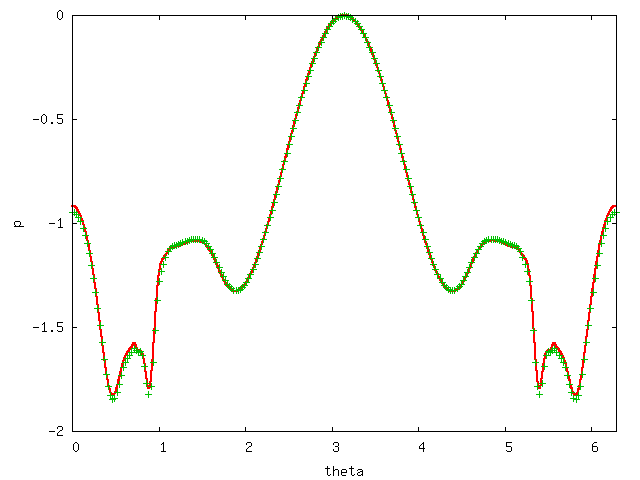
Figure 18: Surface pressure $p$ against $\theta$ at $t=2$ for $Re=9500$. $\theta$ is in radians measured from the rear of the cylinder. The reference value is zero at the front of the cylinder ($\theta=\pi$). Symbols: FDS solution, line: DVM solution.

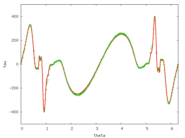
Figure 19: Skin friction against $\theta$ at $t=2$ for $Re=9500$. Symbols: FDS solution, line: DVM solution.

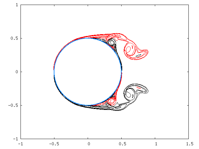
Figure 20: Vorticity contours for $Re=9500$ at $t=2$: black, positive; red, negative. Going from the far field towards the cylinder, the contours are for $|\omega|$=5,10,25,50,100,200. The contours above the axis ($y>0$) are from the DVM code, and those below the axis from the FDS code.

This run generated approximately $8.4\times 10^{5}$ vortex element by $t=3$, a similar number to that used by Koumoutsakos and Leonard [10]. For comparison, for $Re=150$ (Figures 6-10), there were approximately $9.5\times 10^{4}$ vortex elements at $t=3$.

9 Flow past a square.

There is relatively little data available for flow past a square as compared to that for a cylinder. However, plots of drag and vorticity contours are given in [14] for an impulsive start with $Re=100$ and the square at 15^∘ angle of attack. A similar calculation was performed, using a uniform, body fitted, Cartesian grid embedded in a uniform Cartesian grid aligned the flow. Eighty one constant length vortex panels were used on each side of the body, and a grid step of $h=1/81$ was used for both the inner outer grids. The change between the inner and outer grids occurred a distance 0.5 from the body. The time step was $\Delta t=0.005$, giving $h_{v}/h\approx 0.57$. With this set of parameters, the behaviour of the impulse early in the calculation was as expected.

The flow at a right angled convex corner is singular, but both the pressure and the vorticity behaving as $\rho^{-0.456}$ where $\rho$ is the distance from the corner [17]. Hence, there may be large errors in the surface pressure obtained by integrating the panel strengths, and in calculating the lift and drag from the surface forces. Figure 21 shows the drag and lift obtained from both methods. There is reasonable agreement, given the potential for large errors. The drag is consistent with that given in [14]. A calculation with 41 panels on each side of the square and $h=1/41$ produced a similar result to that shown in Figure 21, but with a larger difference between the drag and lift calculated from the impulse and the surface forces.

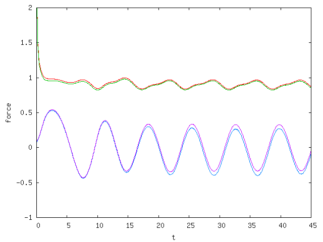
Figure 21: Lift and drag for impulsively started flow past a square at 15^∘ and $Re=100$. The top two lines are the drag, with the upper one from impulse and the lower from the surface forces. The bottom two lines are the lift, with the lower from the impulse and the upper from the surface forces.

Vorticity contours for for $t=20$ are shown in Figure 22. This figure agrees well with that in [14], in particular, as regards the position and strength of the vortices downstream of the body.

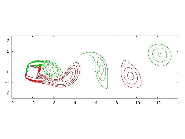
Figure 22: Vorticity contours at $t=20$ for impulsively started flow past a square at 15^∘ and Re=100. A step of 0.5 is used with zero omitted.

In [14], the corners of the square were rounded to avoid unspecified numerical problems. This was not required for the calculations performed in the current work.

10 DVM scheme with a single grid.

All of the calculations described above have used a boundary fitted redistribution mesh near the body and a regular Cartesian mesh further away. Care has been taken to ensure that the total circulation is conserved. An alternative approach, used in a number of previous studies (e.g. [12, 9, 14]), is to delete any vorticity that crosses the boundary and rely on the creation process to regenerate the vorticity in an appropriate manner. There are several advantages to this approach. In particular, it allows simulation for flow past bodies of an arbitrary shape by embedding them into a regular grid, and simply deleting any vortex elements which are redistributed into the body. The major disadvantage is that the method will no longer produce high resolution values for the surface forces. In particular, since part of the circulation in the vortex sheet arises from the non conservative nature of the redistribution at the surface of the body, the surface pressure cannot be estimated using (41) unless the deletion is accounted for.

Simulations were performed using a circular cylinder embedded in a uniform Cartesian grid. Following [9], the vortex elements created each time step were placed a distance of $1.12\sigma$ above the surface so that the maximum velocity generated by a new element occurs at the surface, while all vortex elements within this distance or below the surface were deleted after the redistribution.

The drag for a flow with $Re=150$, 400 vortex panels, a time step of $\Delta t=0.005$ and a redistribution mesh with $h=0.01$ is shown in Figure 23. Also shown is the drag from the FDS scheme, showing good agreement with the DVM values. The vorticity distribution for both methods at $t=1$ is shown in Figure 24. Overall there is very close agreement, although some differences can be seen near the surface. However, and as expected, the distribution of vortex panel strengths and the wall shear stress showed large high frequency oscillations.

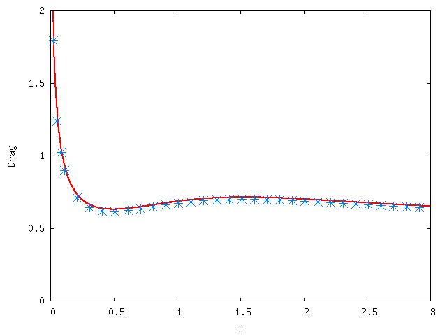
Figure 23: Total drag for impulsively started flow past a circular cylinder at $Re=150$. Line: FDS solution. Symbols: DVM solution using a single Cartesian redistribution grid with $h=0.01$, $\Delta t=0.005$ and 400 vortex panels.

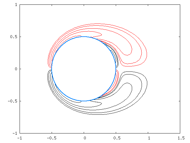
Figure 24: Vorticity contours for $Re=150$ at $t=1$: black, positive; red, negative. Going from the far field towards the cylinder, the contours are for $|\omega|$=1,2,5,10,20. The contours above the axis ($y>0$) are from the DVM code with a single Cartesian redistribution grid with $h=0.01$, $\Delta t=0.005$ and 400 vortex panels, and those below the axis from the FDS code.

A further calculation was performed for $Re=150$ but with 200 panels and $h=0.02$ so that there were approximately quarter the number of vortex elements. The drag was almost the same as shown in Figure 23. The vorticity contours at $t=1$ for both the DVM and FDS schemes are shown in Figure 25. Away from the body there is still good agreement between the two solutions but the lack of resolution near the surface with the DVM method is more apparent.

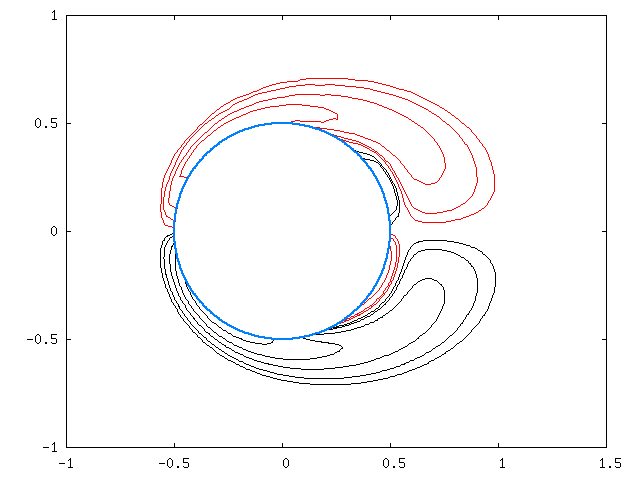
Figure 25: Vorticity contours for $Re=150$ at $t=1$: black, positive; red, negative. Going from the far field towards the cylinder, the contours are for $|\omega|$=1,2,5,10,20. The contours above the axis ($y>0$) are from the DVM code with a single Cartesian redistribution grid with $h=0.02$, $\Delta t=0.02$ and 200 vortex panels, and those below the axis from the FDS code.

Calculations were also performed for flow with $Re=9500$. Figure 26 shows the drag for the FDS method and the DVM scheme with two different resolutions. The better resolved DVM calculation has $N=3000$, $h=1/1000$ and $\Delta t=0.005$, and the coarser calculation $N=1600$, $h=1/400$ and $\Delta t=0.02$. In both cases, the redistribution grid step was chosen to approximately match the vortex panel length. The drag from the better resolved DVM solution shows good agreement with that from the FDS method, except, unsurprisingly, during the very early part of the run. The drag from the coarser calculation also agrees well up to $t\approx 1.5$, but not at later times.

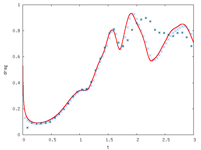
Figure 26: Total drag for impulsively started flow past a circular cylinder at $Re=9500$. Line: FDS solution. Symbols: DVM solutions using a single Cartesian redistribution grid: $\times$, 3000 panels, $h=1/1000$ and $\Delta t=0.005$; $*$, 1600 panels, $h=1/400$ and $\Delta t=0.02$.

Figure 27 shows vorticity contours from both the FDS method and the DVM calculation with the finer grid. There is good agreement, but not as close as with the body fitted grid (Figure 20). A similar comparison with the lower resolution DVM solution showed a similar general structure (e.g. the position of the large vortices sitting off the surface) but significant differences at smaller scales, reflecting a lack of resolution.

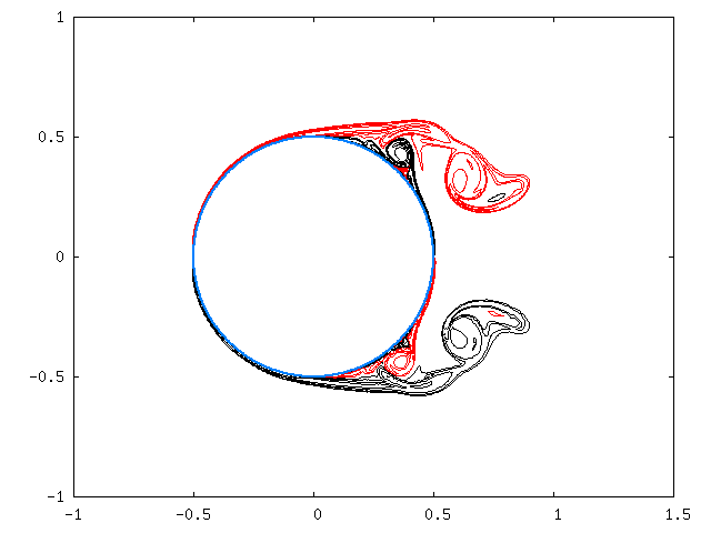
Figure 27: Vorticity contours for $Re=9500$ at $t=2$: black, positive; red, negative. Going from the far field towards the cylinder, the contours are for $|\omega|$=5,10,25,50,100,200. The contours above the axis ($y>0$) are from the DVM code with a single Cartesian redistribution grid with 3000 vortex panels, $h=1/1000$, $\Delta t=0.005$, and those below the axis from the FDS code.

11 Conclusions

A simple redistribution scheme for viscous flow has been presented. Unlike other redistribution schemes, it operates by redistributing the circulation in a vortex element to a set of fixed nodes rather than transferring circulation between vortex elements. A new distribution of vortex elements can then be constructed from the circulation on the nodes. A major advantage of the scheme is that the solution of the redistribution problem is given explicitly by a set of simple algebraic equations. A further advantage is that core overlap is not an issue for the viscous solution.

The scheme will be stable provided the viscous diffusion length is less than the smallest mesh length in the problem. This restriction is similar to that found with other redistribution schemes.

The ability of the scheme to produce high resolution solutions has been demonstrated through a series of test problems. Accurate estimates for both the total body and pointwise surface forces can be obtained when using a body fitted mesh near the surface of the body. Accurate estimates of the total forces on the body can be obtained when using a non conservative scheme with the body embedded in a Cartesian mesh.

The solution presented for the redistribution problem is the simplest possible which satisfies the equations and has the required symmetry. It would be possible to obtain higher order solutions by extending the the computational stencil and setting higher moments to zero. There is no requirement to use the same mesh throughout the computational domain, and the use of local grid refinement is straightforward. Also, the method extends naturally to three-dimensions.

References

- [1] A.J. Chorin. Numerical study of slightly viscous flow. J. Fluid Mech., 57, 785 (1973).
- [2] P. Degond and S. Mas-Gallic. The weighted particle method for convection-diffusion equations. Math. Comput., 53, 485-526 (1989).
- [3] S. Shankar and L. van Dommelen. A new diffusion procedure for vortex methods. J. Comput. Phys., 127, 88-109 (1996).
- [4] S. Subramaniam. A new mesh-free vortex method. PhD thesis, Florida State University, 1996.
- [5] I. Lakkis and A. Ghoniem. A high resolution spatially adaptive vortex method for separating flows. Part I: two-dimensional domains. J. Comp. Phys, 228, 491-515 (2009).
- [6] G.-H. Cottet and P.D. Koumoutsakos. Vortex Methods: Theory and Practice. Cambridge University Press, 2000.
- [7] K. Takeda, O.R. Tutty and A.D. Fitt. A comparison of four viscous models for the discrete vortex method. AIAA 13th Computational Fluid Dynamics Meeting, Colorado, July 1997. AIAA paper 97-1977, 11pp.
- [8] P.A. Smith and P.K. Stansby. Impulsively started flow around a circular cylinder by the vortex method. J. Fluid Mech., 194, 45-77 (1988).
- [9] N.R. Clarke and O.R. Tutty. Construction and Validation of a discrete vortex method for the two-dimensional incompressible Navier-Stokes equations. Computers & Fluids, 23, 751-783 (1994).
- [10] P. Koumoutsakos and A. Leonard. High-resolution simulations of the flow around an impulsively started cylinder using vortex methods. J. Fluid Mech., 296, 1-38 (1995).
- [11] B.D. Bunday. Basic Linear Programming, Edward Arnold (London) (1984).
- [12] P.R. Spalart. Vortex methods for separated flows. Von Karman Inst. for Fluid Mechanics, Lecture Series 1988-05 (1988).
- [13] J.C. Wu. Theory for aerodynamic force and moment in viscous flow. AIAA J., 19, 432-441 (1981).
- [14] P. Ploumhans and G.S. Winckelmans. Vortex methods for high-resolution simulations of viscous flow past bluff bodies of general geometry. J. Comp. Phys, 165, 354-406 (2000).
- [15] M. Bar-Lev and H.T. Yang. Initial flow field over an impulsively started circular cylinder. J. Fluid Mech., 72, 625-647 (1975).
- [16] S.C.R. Dennis and S. Kocabiyik. An asymptotic matching condition for unsteady boundary-layer flows governed by the Navier-Stokes equations. IMA J. Appl. Maths, 47, 81-98 (1991).
- [17] H.K. Moffat. Viscous and restive eddies near a sharp corner. J. Fluid Mech., 18, 1-18 (1964).