Side-entrainment in a jet embedded in a sidewind

Abstract

Numerical simulations of HH jets never show side-entrainment of environmental material into the jet beam. This is because the bow shock associated with the jet head pushes the surrounding environment into a dense shell, which is never in direct contact with the sides of the jet beam. We present 3D simulations in which a side-streaming motion (representing the motion of the outflow source through the surrounding medium) pushes the post-bow shock shell into direct contact with the jet beam. This is a possible mechanism for modelling well collimated “molecular jets” as an atomic/ionic flow which entrains molecules initially present only in the surrounding environment.

1. Introduction

Models of entrainment of molecular, environmental material, in the wings of bow shocks (associated with working surfaces in jets from young stars), are successful in explaining the limb-brightened, cavity-like molecular outflows (at least in a qualitative way). Analytic (Masson & Chernin, 1993; Raga & Cabrit, 1993) and numerical (Raga et al., 1995; Lim et al., 2001) models of this so-called “prompt entrainment” scenario produce limb-brightened molecular structures that resemble the cavity-lile morphologies observed in objects such as the L1157 outflow (e. g., Beltrán et al., 2004).

However, some outflows from young stars also show high-velocity, collimated, jet-like molecular structures. An example of this kind of structure is observed in HH212 (e. g., Codella et al., 2007). These jet-like molecular outflows have been successfully modeled by assuming that the jet itself is initially molecular (e. g., Völker et al., 1999; Lim et al., 2001; Moraghan et al., 2006).

Could these “molecular jets” be the result of environmental molecular gas being entrained into an atomic/ionic jet? The possibility of having “side entrainment” of molecular material has been studied analytically (Cantó & Raga, 1991) and numerically (Taylor & Raga, 1995; Lim et al., 1999). These models show that if one has a fast, atomic jet beam in direct contact (through the sides of the beam) with a molecular environment, a substantial amount of molecular material is indeed entrained into the fast flow.

However, if one computes full simulations of a jet flow, the leading bow shock pushes aside the molecular environment, so that the sides of the jet beam are never in direct contact with the molecular gas. Therefore, the situation necessary for producing side-entrainment of molecular gas (see Taylor & Raga, 1995; Lim et al., 1999) is not obtained.

In the present paper, we study the possibility of overcoming this problem by having a low velocity side-motion of the environment relative to the jet source. This side-wind could represent the motion of the jet source within the surrounding environment. The qualitative effect of the sidewind is described in §2. We have then computed a set of 3D simulations of a radiative jet in a sidewind (§3), producing a variety of flow morphologies (§4). From the resulting flows we compute the amount of environmental material which is pushed by the jet flow (§5) and analyze how much material is actually entrained into the jet beam itself (§6). We finally illustrate the dependence of our results on the resolution of the numerical simulations (§7). The results are summarized in §8.

2. Jet in a sidewind

The main problem when trying to incorporate molecular, environmental material, into a collimated jet is that the leading head of the jet, and possibly also any trailing “internal working surfaces”, push away the environmental gas into a dense shell, which follows the shape of the bow shock wings. Because of this, the molecular environmental material never reaches contact with the jet beam, and lateral entrainment of this material into the jet does not occur. This situation is shown in panel a of Figure 1.

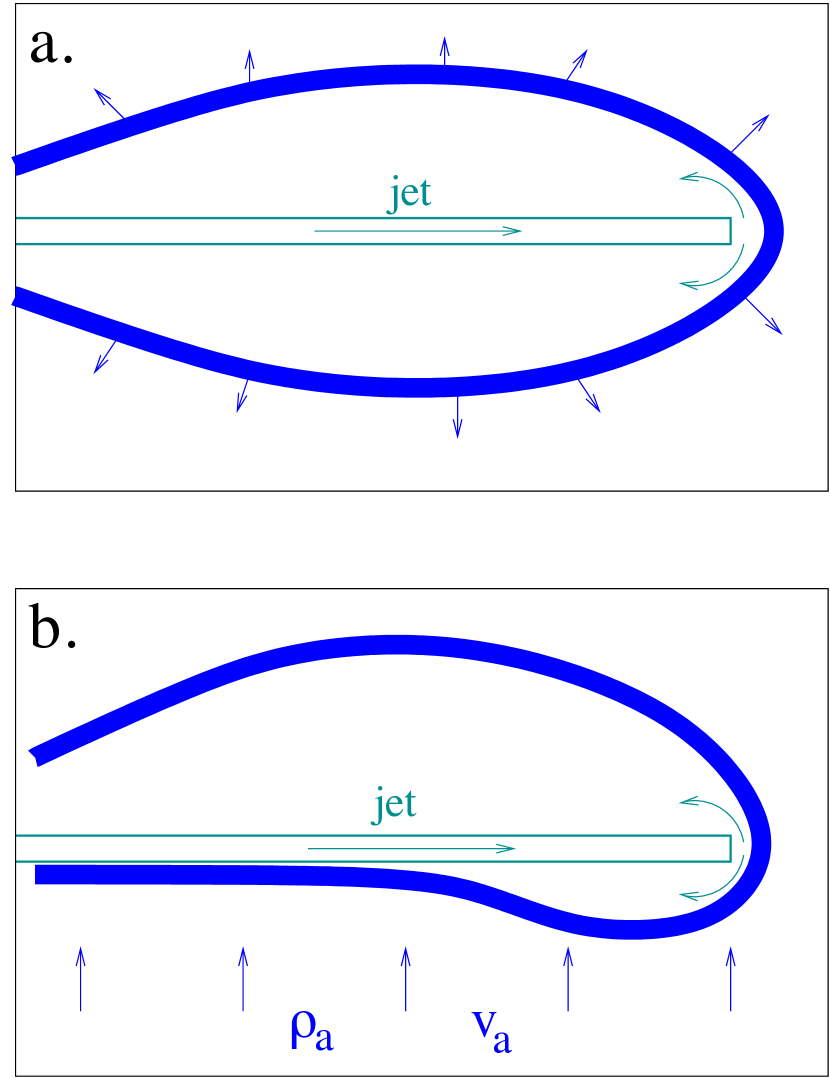
Figure 1.— Schematic diagram showing a jet travelling in a stationary environment (top) and in a sidewind travelling parallel to the ordinate (bottom). The sidewind pushes the dense, post-bow shock shell into direct contact with the jet beam.

It has been suggested that if the dense shell material were warm enough, it might re-expand into the cavity left by the passage of the jet head, and reach contact with the jet beam (see, e. g., Raga & Cabrit, 1993). However, this is found not to be an important effect in jet simulations (see, e.g., Raga et al., 1995; Lim et al., 2001). Possibly, a stratification of the surrounding environment and/or a precession and variability of the jet ejection could lead to the occurrence of side-entrainment into the jet beam (Cabrit et al., 1997). However, ntil now the correct combination of parameters for this to occur has not been found. Other possibilities have been suggested. For example, Lim et al. (2001) studied the survival of molecules (originally present in the environment) in the head of an accelerating jet flow. It is not clear how this high-velocity molecular gas in the jet head could end up being entrained into the jet beam. Another possibility was suggested by Raga et al. (2003), who proposed that the existence of small, dense, moving clumps within the environment might be a way of introducing molecular material into the jet beam. However, it is not clear that this mechanism leads to molecular emission structures that resemble the observations.

The possibility that we study in this paper is that the presence of a side-streaming environment pushes the bow shock wing (and the post-bow shock, dense shell) against the jet beam, as shown in panel b. of Figure 1. The side-streaming could be the result of the motion of the jet source through the molecular cloud, and would have velocities of at most a few km s^-1. Both analytic (Cantó & Raga, 1995; Raga et al., 2009a) and numerical (Lim & Raga, 1998; Masciadri & Raga, 2001; Ciardi et al., 2008) models of jets in sidewinds have been computed previously. These models have mostly been applied to jets within expanding H II regions (Ciardi et al., 2008) or to jets embedded in an isotropic stellar wind (Raga et al., 2009a). The relatively high sidewind velocities relevant for these cases ($\sim 10$-30 km s^-1 for an expanding H II region and up to $\sim 1000$ km s^-1 for a stellar wind), can produce jets with strongly curved jet beams.

For lower sidewind velocities (not studied in the papers cited above), only a weak curvature will be produced as a result of the jet/sidewind interaction. However, the bow shock wing will still be pushed against the body of the jet, as shown in the schematic diagram of Figure 1. We focus on this regime, in which the dense shell of swept up environmental material is pushed into contact with the body of the jet beam (therefore allowing the entrainment of environmental gas into the beam), but a relatively straight jet path is still obtained. The numerical simulations which we have carried out are described in the next section.

3. The numerical simulations

We have computed a set of 3D gasdynamic simulations of jet/sidewind interactions. All of them have been computed in a $(2,0.5,0.5)\times 10^{17}$ cm cartesian grid. The jet is injected at $x=0$ (in the centre of the boundary plane of the computational grid), with a velocity parallel to the $x$-axis. A sidewind is injected in the $y=0$ plane, with a velocity directed along the $y$-axis. A reflection boundary condition is applied on the $x=0$ boundary outside the jet beam, and transmission conditions are applied on all of the other boundaries except the $y=0$ plane (in which the sidewind is injected).

An initially neutral, top-hat jet of velocity $v_{j}$, density $n_{j}$, radius $r_{j}=10^{15}$ cm and temperature $T_{j}=10^{3}$ K moves into an initially uniform, neutral environment with a density $n_{a}=200$ cm^-3, temperature $T_{a}=10$ K and sidestreaming velocity $v_{a}$. A set of models with different values of $v_{j}$, $n_{j}$ and $v_{a}$ has been computed, with the parameters given in Table 1.

Table 1Model characteristics.

Model	$v_{j}$	$v_{a}$	$n_{j}$
	[km s-1]	[km s-1]	[cm-3]	resolution
a1	150	02	1000	lr,mr,hr
b1	150	05	1000	mr
c1	150	10	1000	lr,mr,hr
a2	300	02	1000	mr
b2	300	05	1000	mr
c2	300	10	1000	mr
a3	150	02	5000	mr
b3	150	05	5000	mr
c3	150	10	5000	mr

The simulations were carried out with the “Yguazú-a” code (Raga et al., 2000), solving the 3D gasdynamic equations together with a continuity/rate equation for neutral H. The parametrized cooling function described by Raga et al. (2009b) is included in the energy equation. Also, we integrate an equation for a normalized passive scalar $g$ with which we distinguish between the ambient and jet medium. If the scalar was positive it indicated that the material was initially medium material, while if it was negative it was jet material. For example, if we had only ambient medium material $g=1$, or if we had pure jet material $g=-1$. With the use of this scalar we were able to calculate the amount of mixing between the ambient medium and the jet material. For this, we defined the mixing mass fraction as $f_{m}=(g+1)/2$. It is clear that for pure ambient medium $f_{m}=1$; while for pure jet material $f_{m}=0$, intermediate values of $f_{m}$ indicates that there was material from both the ambient medium and the jet mixed together. The case in which we have 99% ambient medium mixed with 1% of jet material ($f_{m}=0.99$), is defined as “99% mixing fraction”; while the 1% ambient medium case ($f_{m}=0.01$) as “1% mixing fraction”.

A 6-level binary adaptive grid has been used with three different maximum resolutions $\Delta x=3.91$, 1.95 and $0.98\times 10^{13}$ cm (along the three axes). We have called these the “low”, “medium” and “high” resolutions (labeled in Table 1 with letters lr, mr and hr, respectively).

4. The resulting flow stratifications

As an example of the flows resulting from our simulations, in Figure 2 we show $xy$-cuts showing the time-evolution of the mid-plane density stratification obtained from model a1 (see Table 1). This figure also shows 2 contours, corresponding to the 99% mixing fraction ($f_{m}=0.99$, outer contour), and 1% mixing fraction ($f_{m}=0.01$, inner contour).

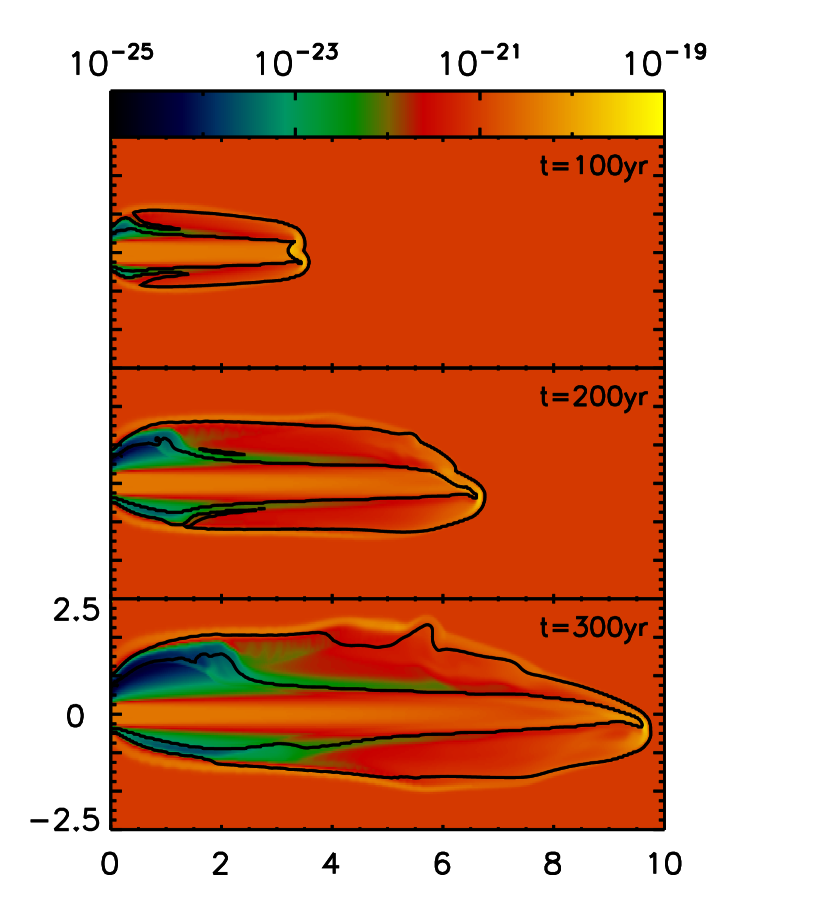
Figure 2.— Density stratifications (color scale, given in g cm^-3 by the top bar) and mixing fractions (contours) obtained from model a1 (see Table 1). The side-streaming environment flows along the vertical axis of the plots. The displayed stratifications correspond to cuts on a plane that includes the outflow axis and the sidewind, at integration times $t=100$ (top), 200 and 300 yr (bottom). The two contours correspond to the 99 % mixing fraction ($f_{m}=0.99$, outer contour); and the 1 % mixing fraction case ($f_{m}=0.01$, inner contour). The axes are labeled in units of $10^{16}$ cm.

In model a1, the $xy$-cuts show a side-to-side asymmetry that is a direct result of the fact that the environment is flowing along the $+y$-direction. This asymmetry is seen as a distortion of the leading bow shock, and as a penetration of environmental material to regions close to the jet beam in the up-sidewind ($-y$) direction.

In Figure 3, we show single time frames of the $xy$-midplane density stratifications obtained from the 9 models of Table 1. In each of the three columns of Figure 3 (from top to bottom), we see the effect of increasing velocity of the sidewind (the top, centre and bottom frames correspond to $v_{a}=2$, 5 and 10 km s^-1, respectively, see Table 1). It is clear that for higher values of $v_{a}$, the environmental material penetrates more strongly towards the jet beam in the up-sidewind region.

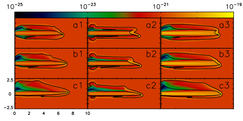
Figure 3.— Density stratifications (color scale, given in g cm^-3 by the top bar) and mixing fractions (contours) obtained for the models listed in Table 1. The displayed stratifications correspond to cuts on a plane that includes the outflow axis and the sidewind, at integration times $t=200$ yr (for models a1, b1, c1, a3, b3 and c3) or $t=100$ yr (for models a2, b2, c2). The two contours correspond to the 99 % mixing fraction ($f_{m}=0.99$, outer contour); and the 1 % mixing fraction case ($f_{m}=0.01$, inner contour). The axes are labeled in units of $10^{16}$ cm.

A comparison of the first and second columns of Figure 3 shows that if one increases the jet velocity from $v_{j}=150$ km s^-1 (models a1, b1 and c1) to 300 km s^-1 (models a2, b2 and c2, see Table 1) the resulting density stratifications and mixing fractions remain qualitatively unchanged, showing slightly more pronounced asymmetries for the higher jet velocity. In particular, it is clear that in regions close to the source the post-bow shock dense shell touches the jet beam in all of the $v_{a}=10$ km s^-1 models (bottom row of Figure 3).

Finally, we also see that if one increases the jet density (from $n_{j}=1000$ cm^-3 for the models in the first column to 5000 cm^-3 for the models in the third column, see Table 1), less penetration of the environmental material into the jet beam is obtained. This effect can be seen as broader 99% pure jet material regions (limited by the inner contour) in the a3, b3, c3 models (compared to a1, b1 and c1).

5. Entrained material

As we have described in §3, from our simulations we obtain the environmental to total mass mixing fraction $f_{m}$ as a function of position and time. Using this mixing fraction, we compute the jet mass loss rate associated with motions along the $x$-axis :

$${\dot{M}}_{j}(x)=\int\int\left[1-f_{m}\right]\rho u\,dy\,dz\,,$$ (1)

and the mass rate of the entrained material

$${\dot{M}}_{AM}(x)=\int\int f_{m}\rho u\,dy\,dz\,,$$ (2)

where $f_{m}$, $\rho$ and $u$ are the 3D mixing fraction, density and $x$-velocity (respectively), obtained for a given integration time $t$.

The mass loss rates obtained in this way for models a1 and c1 are shown in Figure 4 and 5 (for times $t=50$ to 300 yr). It must be noted that calculating the position of the jet head was not trivial, it required fine-tuning, was not obtained exactly the same for each model, and the environmental mass rate from the entrained material (${\dot{M}}_{AM}$) was extremely sensitive to it. Thus, in order to be consistent in our analysis, we exclude the head of the jet from our discussion. For model a1 (which has a $v_{a}=2$ km s^-1 sidewind, see Table 1), we see that, at all times ${\dot{M}}_{AM}$ monotonically grows along the jet axis, and that a maximum is reached at the position of the jets head (top panel of Figure 4). For this model, the ${\dot{M}}_{AM}/{\dot{M}}_{j}$ ratio also grows with distance $x$ from the source, having values of $\sim 5\to 8\times 10^{-3}$ at the middle of the length of the jet (at a given integration time), and reaching values of $\sim 1$ at the head of the jet (bottom panel of Figure 4).

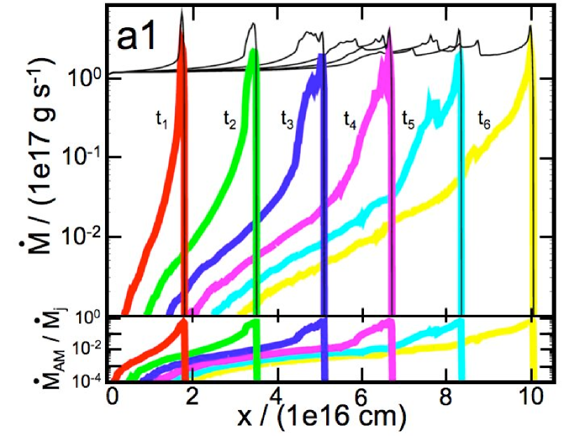
Figure 4.— Top panel: Mass rates associated with the jet (${\dot{M}}_{j}$, black lines) and environmental material (${\dot{M}}_{AM}$, coloured lines) as a function of position $x$ along the outflow axis, obtained from the flow stratifications of model a1 (see Table 1) at integration times $t_{1}=50$ (red lines), $t_{2}=100$ (green), $t_{3}=150$ (blue), $t_{4}=200$ (pink), $t_{5}=250$ (cyan) and $t_{6}=300$ yr (yellow). Bottom panel: the ${\dot{M}}_{AM}/{\dot{M}}_{j}$ ratio as a function of $x$ for the same integration times.

For model c1 (which has the same parameters as model a1 except for a $v_{a}=10$ km s^-1 sidewind, see Table 1), a qualitatively similar behavior is obtained for the ambient mass rate, but with higher values of ${\dot{M}}_{AM}$ at all times and positions along the jet (top panel of Figure 5). The ${\dot{M}}_{AM}/{\dot{M}}_{j}$ ratio has values of $\sim 1.1\to 1.3\times 10^{-2}$ at the middle of the length of the jet (for all times), a factor of $\sim 2$ larger than the values obtained for model a1 (also except for the head of the jet, which we excluded from the analysis due to lack of consistency).

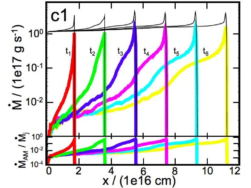
Figure 5.— The same as Figure 4, but for model c1 (see Table 1).

We now calculate the mean velocities associated with the jet and environmental mass rates :

$$\overline{v}_{j}(x)=\frac{1}{{\dot{M}}_{j}(x)}\int\int\left[1-f_{m}\right]\rho u^{2}\,dy\,dz\,,$$ (3)

$$\overline{v}_{AM}(x)=\frac{1}{{\dot{M}}_{AM}(x)}\int\int f_{m}\,\rho u^{2}\,dy\,dz\,,$$ (4)

where ${\dot{M}}_{j}(x)$ and ${\dot{M}}_{AM}$ are given by equations (1) and (2).

The mean velocities obtained in this way for models a1 and c1 are shown in Figure 6. We see that the mean forward velocity $\overline{v}_{j}$ of the jet material is of 150 km s^-1 at $x=0$ (correctly coinciding with the injection velocity, see Table 1). For model a1 (top panel of Figure 6), the jet velocity drops close to the position of the head to $\sim 120$ km s^-1. The drop in $\overline{v}_{j}$ occurs closer to the jet source in model c1 (bottom panel of Figure 6). In both models (a1 and c1), the mean forward velocity $\overline{v}_{AM}$ of the environmental material grows along the length of the outflow, with a velocity of $\approx 120$ km s^-1 at the jet head. At all times, we also see a peak in $\overline{v}_{AM}$ at $x<10^{16}$ cm (the position of this peak being at larger distances from the source for longer integration times). This peak is associated with a region (close to the jet source) in which the post-bow shock shell touches the jet beam since early evolutionary times (see Figure 2).

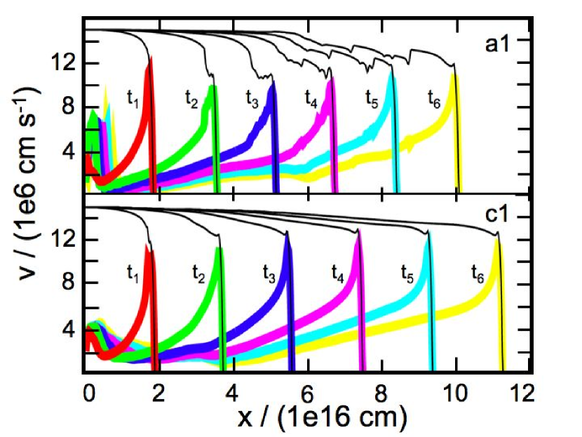
Figure 6.— Top panel: Average velocity associated with the jet ($\overline{v}_{j}$, black lines) and the environmental material ($\overline{v}_{AM}$, coloured lines) as a function of position $x$ along the outflow axis, obtained from the flow stratifications of model a1 (see Table 1) at integration times $t_{1}=50$ (red lines), $t_{2}=100$ (green), $t_{3}=150$ (blue), $t_{4}=200$ (pink), $t_{5}=250$ (cyan) and $t_{6}=300$ yr (yellow). Bottom panel: The same as in the top panel, but for model c1 (see Table 1).

In Figure 7, we show the environmental mass rate as a function of distance from the source obtained from all of the models of Table 1 (only the results for a single integration time are shown for each model). All of the models give ${\dot{M}}_{AM}\approx 10^{17}$ g s^-1 close to the head of the jet. Lower mass loss rates are obtained closer to the outflow source.

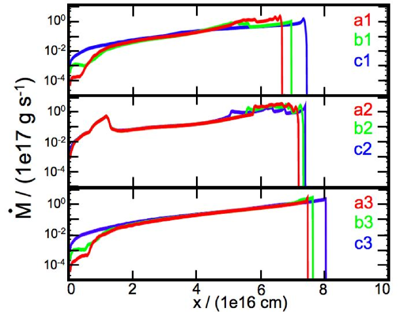
Figure 7.— Environmental mass rate ${\dot{M}}_{AM}$ (see equation 2) computed for all models (see Table 1) for an integration time of 200 yr for models a1, b1, c1, a3, b3 and c3 and of 100 yr for models a2, b2 and c2.

The models with $v_{j}=300$ km s^-1 (a2, b2 and c2, central panel) show basically identical ${\dot{M}}_{AM}(x)$ dependencies for $x<5\times 10^{16}$ cm, and a clear spike at $x_{sp}\approx 10^{16}$ cm, but as we shall see corresponds to environmental material which is not entrained primarily by the sidewind, but rather from the leading bow-shock, thus is not of interest for this study. The $v_{j}=150$ km s^-1 models (top and bottom panels) show a region close to the outflow source (with $x<2\times 10^{16}$ cm) in which larger ${\dot{M}}_{AM}$ are obtained for larger sidewind velocities ($v_{a}=2$ km s^-1 for models a1 and a3, 5 km s^-1 for b1 and b3 and 10 km s^-1 for c1 and c3, see Table 1). As we will see in the following section, in this region we are seeing environmental material that is directly entrained into the jet beam (due to the presence of the sidewind).

Figure 8 shows the environmental mean velocity ($\overline{v}_{AM}$, see equation 4), as a function of position for all of the computed models (see Table 1). In the $v_{j}=150$ km s^-1 models (upper and lower panels of Figure 8), regardless of the sidewind velocity the correspondent $\overline{v}_{AM}$ grows from low ($\sim 1$ km s^-1) close to the source, up to values comparable to the jet velocity ($\sim 250$ km s^-1) at the head of the jet.

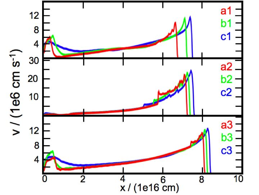
Figure 8.— Environmental average velocity ($\overline{v}_{AM}$) (see equation 4) computed for all models (see Table 1) for an integration time of 200 yr for models a1, b1, c1, a3, b3 and c3 and of 100 yr for models a2, b2 and c2.

Very similar results are obtained for the models with $v_{j}=300$ km s^-1 (central panel), except for the presence of a spike at $x_{sp}\approx 10^{16}$ cm. Since the corresponding $\overline{v}_{AM}$ at $x_{sp}$ for these models ($\sim 0.03v_{j}$) was lower than that from the models with $v_{j}=150$ km s^-1 (where $\overline{v}_{AM}\sim 0.04-0.20v_{j}$), we had an insight that the material at the spike of Figure 7 (for models with $v_{j}=300$ km s^-1) corresponded to slowly moving material which was mostly entrained by the leading bow-shock and not due to the presence of the sidewind.

Also in Figure 8, there is evidence of “high velocity material . Our models with $v_{j}=150$ km s^-1 showed the presence of a fast region close to the source ($x<2\times 10^{16}$ cm). In this region $\overline{v}_{AM}$ has values of $\sim 40\to 70$ km s^-1 (of order $\sim 50$% of the $v_{j}$). These large $\overline{v}_{AM}$ values close to the source are associated with the direct entrainment of the dense post-bow shock shell into the jet beam due to the sidewind.

6. Fast entrained material

In order to study the environmental material which is directly entrained into the jet beam, we compute the mass rate and average velocity of the environmental material that moves along the jet axis at velocities $>v_{j}/2$ (in other words, with velocities larger than 75 km s^-1 for models a1, b1, c1, a3, b3, c3 and larger than 150 km s^-1 for models a2, b2 and c2). We call these the “high velocity” mass rate ${\dot{M}}_{AM,h}$ and average velocity $\overline{v}_{AM,h}$.

The values of ${\dot{M}}_{AM,h}(x)$ obtained for all models are shown in Figure 9. We see that in the region close to the outflow source ($x<2\times 10^{16}$ cm) the low velocity jet models (with $v_{j}=150$ km s^-1, models a1, b1, c1, a3, b3, c3) have environmental mass rates which monotonically grow with increasing values of the sidewind velocity ($v_{a}$). For $v_{a}=10$ km s^-1 (models c1 and c3), the mass rate in this region has values of ${\dot{M}}_{AM,h}\approx 5\times 10^{14}$ g s^-1, of the order of $\sim 0.5$% of the mass loss rate of the jet. Lower values of ${\dot{M}}_{AM,h}$ are obtained for the $v_{a}=5$ (b1 and b3) and $v_{a}=2$ km s^-1 models (a1 and a3). Finally, we see that the values of ${\dot{M}}_{AM,h}$ in the region close to the source are much lower (${\dot{M}}_{AM,h}\approx 5\times 10^{13}$ g s^-1) for the $v_{j}=300$ km s^-1 models (a2, b2, c2, central panel of Figure 9). This confirms the fact that the material from the spike in Figure 7 (for models with $v_{j}=150$ km s^-1), corresponds to environmental material which was not entrained in its majority by the sidewind (and so, is not of interest for this study).

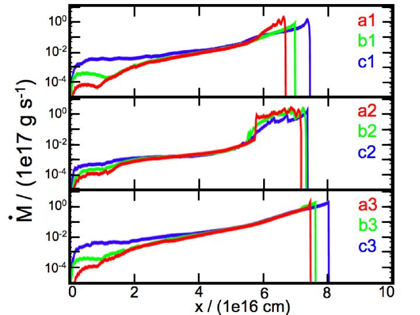
Figure 9.— Mass rate of the environmental material which moves with “high” velocities along the jet axis (${\dot{M}}_{AM,h}$). For model a1, b1, c1, a3, b3, c3 we show the material that is moving with $\overline{v}_{AM}>$75 km s^-1, and with $\overline{v}_{AM}>$150 km s^-1 for models a2, b2 and c2.

All of the models show a strongly increasing ${\dot{M}}_{AM,h}(x)$ for $x>2\times 10^{16}$ cm. This growth is associated with the fact that the motion of the post-bow shock shell becomes progressively more forward directed as we approach the head of the jet.

Therefore, there are two components of the fast (with axial velocities $>v_{j}/2$) ambient material :

• material originating in the region in which the post-bow shock shell is in contact with the jet beam,

• material in the post-bow shock shell in the region close to the jet head.

The spatial distribution of these two components is shown in Figure 10, with the mid-plane spatial distribution of the density $\rho f_{m}$ of the fast ($v_{x}>v_{j}/2$) ambient material obtained from models a1 and c1 (for an integration time of 300 yr). These stratifications show that the fast ambient material is confined to a region within or in near contact to the jet beam.

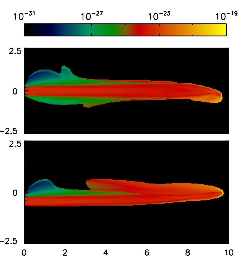
Figure 10.— Environmental mass fraction times the density stratification ($\rho\times f_{m}$, colour scale, given in g cm^-3 by the top bar), of the fast ambient material obtained from models a1 (top panel) and c1 (bottom panel), for an integration time of 300 yr. The axes are labeled in units of $10^{16}$ cm.

7. A resolution study

In order to illustrate the effect of the numerical resolution, we have computed two of the models (a1 and c1, see Table 1) at three resolutions: $\Delta x=3.91$, 1.95 and $0.98\times 10^{13}$ cm (along the three axes). In Figure 11, we show the density stratifications obtained from model a1 at these three resolutions, for a $t=200$ yr integration time.

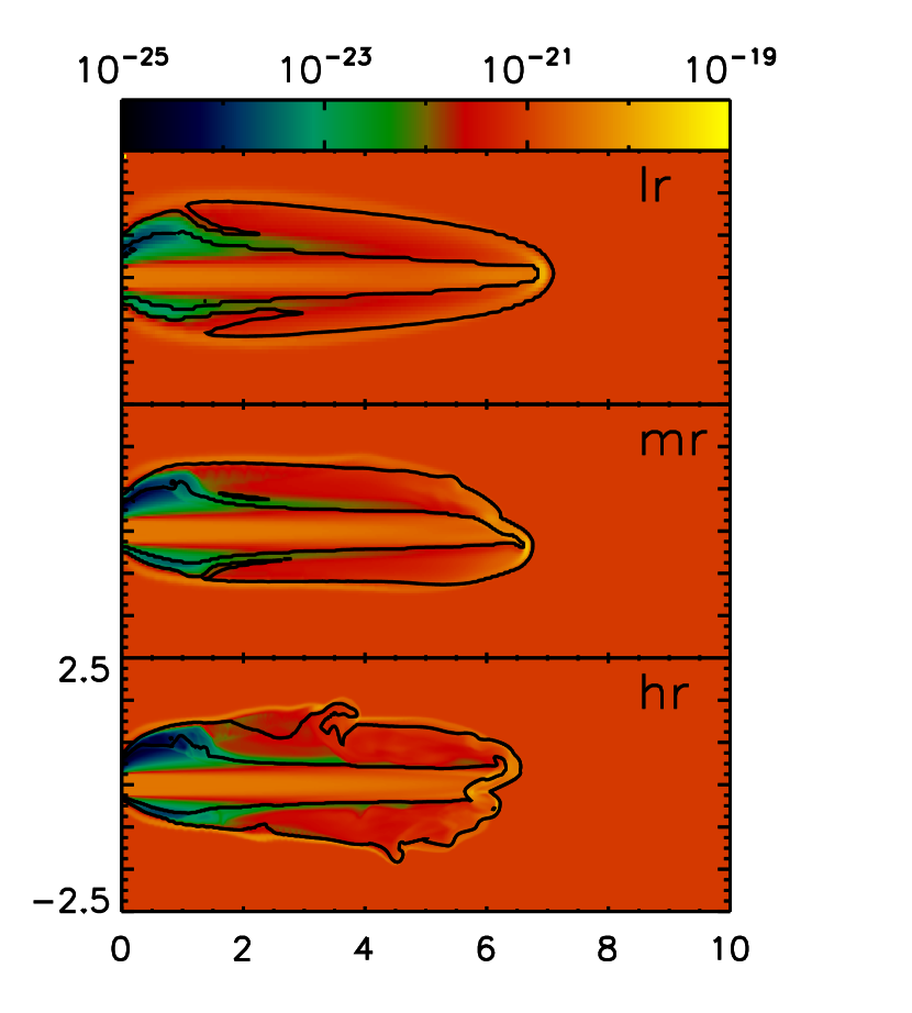
Figure 11.— Density stratifications (color scale, given in g cm^-3 by the top bar) and mixing fractions (contours) obtained from model a1 at three different resolutions for an integration time of 200 yr (see Table 1). The two contours correspond to the 99 % mixing fraction ($f_{m}=0.99$, outer contour); and the 1 % mixing fraction case ($f_{m}=0.01$, inner contour). The axes are labeled in units of $10^{16}$ cm. The three panels correspond to “low” (case in which $\Delta x=3.91\times 10^{13}$ cm along the three axes, top panel), “medium” ($\Delta x=1.95\times 10^{13}$ cm), and “high” ($\Delta x=0.98\times 10^{13}$ cm, bottom panel) resolutions.

It is clear that more complex structures are obtained for increasing resolutions. However, the result that the post-bow shock shell is swept into contact with the jet beam (as a result of the side-streaming environment) is present at all resolutions (see Figure 11). Therefore, side-entrainment into the jet beam occurs regardless of the resolution of the simulations.

In Figure 12, we show the total environmental mass rate (${\dot{M}}_{AM}$, top frame) and the mass rate of the fast entrained material (${\dot{M}}_{AM,h}$, bottom frame) as a function of distance from the source, computed from the $t=200$ yr stratification of model a1. The values of ${\dot{M}}_{AM}$ and ${\dot{M}}_{AM,h}$ are similar at all resolutions in the region close to the jet head.

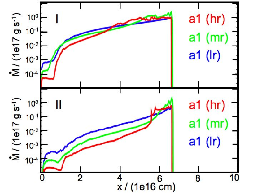
Figure 12.— Total environmental mass rate (${\dot{M}}_{AM}$, top panel) and the mass rate of the fast entrained material (${\dot{M}}_{AM,h}$, bottom panel), as a function of distance from the source, computed for the three different resolutions from model a1 (at an integration time $t=200$ yr).

On the other hand, in the region close to the source (where the dense, post-bow shock shell is being entrained into the jet beam), the environmental mass rate shows a stronger dependence on the resolution. In particular, we have a factor of $\sim 10$ decrease in ${\dot{M}}_{AM,h}$ for a factor of 4 increase in the resolution of the simulation. This result is to be expected (given the lower numerical diffusion of the higher resolution simulations), and its implications are discussed in the following section.

It is clear that in this resolution study a relatively small range (of a single octave) of resolutions is explored. This is a result of the fact that simulations with less than $\sim 10$ grid points across the jet beam are basically meaningless, and that our highest resolution simulation (model hr) resolves the jet beam diameter with $\sim 100$ points (at the highest resolution of the adaptive grid). This resolution is “competitive” in terms of recent 3D astrophysical jet simulations, for example Rossi et al. (2008) computed 3D simulations of entrainment in relativistic jets resolving the jet diameter with $\sim 20$ points). In the near future we will be able to carry out 3D simulations with higher resolutions, hopefully reaching $\sim 300-500$ points across the jet diameter. This will extend the range in resolutions to $\sim 1.5$ octaves (which is still not very impressive).

The situation is therefore somewhat hopeless. If we take the number of grid points across the jet diameter as an estimate of the Reynolds number of the simulation, we see that at the present time we can only expect to reach Re$\sim 500$. Such Reynolds numbers are $\sim 2$ orders of magnitude below the Reynolds number (of $\sim 50000$) necessary to reach the “high Re” regime, in which the entrainment rate becomes independent of Re (Birch & Eggers, 1972). Therefore, it is unclear if this “high Re” regime (relevant for astrophysical jets) will ever be reached by 3D gasdynamic simulations. Regardless of this fact, exploring the development of the Kelvin-Helmholtz instabilities (that initiate the turbulent entrainment) at increasing spatial resolutions is probably still a worthwhile pursuit. Different efforts in this direction have been done by Micono et al. (2000a, b); Xu et al. (2000); Rosen & Hardee (2002).

An eventually more fruitful approach might be to incorporate a “turbulence parametrization scheme”, which has to be calibrated with laboratory experiments in order to provide the correct mass entrainment rate. The application to astrophysical jets of a simple, “$\alpha$-model” turbulence parametrization was discussed by Cantó & Raga (1991). A more evolved, “k-$\epsilon$” scheme was explored by Falle (1994).

The problem of this approach of course is that the turbulence parametrization schemes are normally calibrated with non-radiative, laboratory jet flow experiments. Therefore, it is not clear whether or not the resulting parametrization is appropriate for modeling the entrainment in radiative jets. A possible solution to this problem would be to attempt to calibrate turbulence parametrization schemes with newly available experiments of radiative plasma jets (see, e. g. Ampleford et al., 2008). The relevant experimental data, however, are still not available.

8. Conclusions

It has been suggested that the molecular emission observed along well collimated, jet-like outflows from young stars might be the result of entrainment of molecular environmental material into the jet beam (Cantó & Raga, 1991). However, this side-entrainment has never been seen in numerical simulations of HH jets, because the environmental material is pushed into a dense, post-bow shock shell which does not touch the jet beam.

In this paper, we present 3D numerical simulations of a jet in a sidewind, with sidewind velocities in the $v_{a}=2\to 10$ km s^-1 range (the lower part of this range being consistent with the peculiar motions of T Tauri stars). We find that for many parameter combinations the sidewind pushes the post-bow shock shell into direct contact with the jet beam (see Figure 2 and 3). In this region of contact, side-entrainment of environmental material into the jet beam does take place.

In our simulations, the side-entrainment results in mass rates ${\dot{M}}_{AM,h}\sim 5\times 10^{14}$ g s^-1, corresponding to $\sim 0.5$ %  of the mass loss rate ${\dot{M}}_{j}$ of the jet (see §5). If the molecular, environmental gas is not dissociated during the process of side-entrainment, this would result in a molecular fraction of $\sim 0.5$ % within the jet beam, which would result in molecular column densities high enough to produce observable molecular emission (Raga et al., 2005).

Our present simulations do not include the chemistry of the entrained material, so that we are not able to see whether or not the molecules in the side-entrained material actually survive the entrainment process. However, the fact that the side-entrained material has been shocked by the slow-moving far bow shock wings, and that the region of contact between the shocked environment and the jet remains cool (at temperatures of $\sim 10^{3}$ K) indicates that molecules indeed might be entrained into the jet beam without being dissociated.

Furthermore, our simulations do not describe correctly the entrainment of the post-bow shock shell into the jet beam. An indication of this is the fact that we obtain entrained mass rates that strongly depend on the spatial resolution of our simulations (see §7). In order to overcome this problem, it will be necessary to go to much higher resolutions, in order to resolve the Kelvin-Helmholtz instabilities that produce the side-entrainment (see e. g Micono et al., 2000a, b), or to use a “turbulence parametrization recipe” (Cantó & Raga, 1991; Falle, 1994).

Even though our simulations do not fully describe the side-entrainment process, they conclusively show that a side-streaming environment (reflecting the motion of the jet source) will push the post-bow shock shell into direct contact with the jet beam. This then provides the conditions in which molecular material will be entrained into the fast jet beam, giving “parmetrized turbulence” jet models -initially suggested for astrophysical jets by Bicknell (1984)-, a new life as a possible explanation for the molecular jets observed in star forming regions.

References

- Ampleford et al. (2008) Ampleford, D. J., et al. 2008, Physical Review Letters, 100, 035001
- Beltrán et al. (2004) Beltrán, M. T., Gueth, F., Guilloteau, S., & Dutrey, A. 2004, A&A, 416, 631
- Bicknell (1984) Bicknell, G. V., ApJ, 286, 68
- Birch & Eggers (1972) Birch, S. F., & Eggers, J. M. 1972, In: Free Turbulent Shear Flows, Conf. Proc. NASA-SP-321, Vol. I, 11-40
- Cabrit et al. (1997) Cabrit, S., Raga, A. C., & Gueth, F. 1997, Herbig-Haro Flows and the Birth of Stars, 182, 163
- Cantó & Raga (1991) Cantó, J., & Raga, A. C. 1991, ApJ, 372, 646
- Cantó & Raga (1995) Cantó, J., & Raga, A. C. 1995, MNRAS, 277, 1120
- Ciardi et al. (2008) Ciardi, A., Ampleford, D. J., Lebedev, S. V., & Stehle, C. 2008, ApJ, 678, 968
- Codella et al. (2007) Codella, C., Cabrit, S., Gueth, F., Cesaroni, R., Bacciotti, F., Lefloch, B., McCaughrean, M. J. 2007, A&A, 462, L53
- Falle (1994) Falle, S. A. E. G. 1994, MNRAS, 269, 607
- Lim & Raga (1998) Lim, A. J., & Raga, A. C. 1998, MNRAS, 298, 871
- Lim et al. (1999) Lim, A. J., Rawlings, J. M. C., & Raga, A. C. 1999, MNRAS, 308, 1126
- Lim et al. (2001) Lim, A. J., Rawlings, J. M. C., & Williams, D. A. 2001, A&A, 376, 336
- Masciadri & Raga (2001) Masciadri, E., & Raga, A. C. 2001, AJ, 121, 408
- Masson & Chernin (1993) Masson, C. R., & Chernin L. M. 1993, ApJ, 414, 230
- Micono et al. (2000a) Micono, M., Bodo, G., Massaglia, S., Rossi, P., Ferrari, A., & Rosner, R. 2000a, A&A, 360, 795
- Micono et al. (2000b) Micono, M., Bodo, G., Massaglia, S., Rossi, P., & Ferrari, A. 2000b, A&A, 364, 318
- Moraghan et al. (2006) Moraghan, A., Smith, M. D., & Rosen, A. 2006, MNRAS, 371, 1448
- Raga & Cabrit (1993) Raga, A. C., & Cabrit, S. 1993, A&A, 278, 267
- Raga et al. (1995) Raga, A. C., Taylor, S. D., Cabrit, S., & Biro, S. 1995, A&A, 278, 267
- Raga et al. (2000) Raga, A. C., Navarro-González, R., & Villagrán-Muniz, M. 2000, RMxAA, 36, 67
- Raga et al. (2003) Raga, A. C., Velázquez, P. F., de Gouveia dal Pino, E. M., Noriega-Crespo, A., & Mininni, P. 2003, RMxAC, 15, 115
- Raga et al. (2005) Raga, A. C., Williams, D. A., & Lim, A. J. 2005, RMxAA, 41, 137
- Raga et al. (2009a) Raga, A. C., Cantó, J., Rodríguez-González, A., & Esquivel, A. 2009a, A&A, 493, 115
- Raga et al. (2009b) Raga, A. C., Henney, W., Vasconcelos, J., Cerqueira, A., Esquivel, A., & Rodríguez-González, A. 2009b, MNRAS, 392, 964
- Rosen & Hardee (2002) Rosen, A., & Hardee, P. E. 2002, New Astron. Rev., 46, 433
- Rossi et al. (2008) Rossi, E. M., Armitage, P. J., & Menou, K. 2008, MNRAS, 391, 922
- Taylor & Raga (1995) Taylor, S. D., & Raga, A. C. 1995, A&A, 296, 823
- Völker et al. (1999) Völker, R., Smith, M. D., Suttner, G., & Yorke,, H. W. 1999, A&A, 343, 953
- Xu et al. (2000) Xu, J., Hardee, P. E., & Stone, J. M. 2000, ApJ, 543, 161