On the relationship between parametric two-electron reduced-density-matrix methods and the coupled electron pair approximation

Abstract

Parametric two-electron reduced-density-matrix (p-2RDM) methods have enjoyed much success in recent years; the methods have been shown to exhibit accuracies greater than coupled cluster with single and double substitutions (CCSD) for both closed- and open-shell ground-state energies, properties, geometric parameters, and harmonic frequencies. The class of methods is herein discussed within the context of the coupled electron pair approximation (CEPA), and several CEPA-like topological factors are presented for use within the p-2RDM framework. The resulting p-2RDM/$n$ methods can be viewed as a density-based generalization of CEPA/$n$ family that are numerically very similar to traditional CEPA methodologies. We cite the important distinction that the obtained energies represent stationary points, facilitating the efficient evaluation of properties and geometric derivatives. The p-2RDM/$n$ formalism is generalized for an equal treatment of exclusion-principle-violating (EPV) diagrams that occur in the occupied and virtual spaces. One of these general topological factors is shown to be identical to that proposed by Kollmar [C. Kollmar, J. Chem. Phys. 125, 084108 (2006)], derived in an effort to approximately enforce the $D$, $Q$, and $G$ conditions for $N$-representability in his size-extensive density matrix functional.

I Introduction

It has long been understood that the ground-state energy for a many-electron system can be expressed as a functional of the two-electron reduced-density-matrix ($2$-RDM) REF:7_Challenge ; REF:7_RDMBook and thus the energy may be determined without knowledge of the $N$-electron wave function. The direct determination of the $2$-RDM cannot be accomplished without imposing the so-called $N$-representability conditions REF:7_Challenge ; REF:7_NREP1 ; REF:7_NREP2 : constraints that guarantee that the $2$-RDM corresponds to a realistic $N$-body density. Two general classes of methods for the determination of the $2$-RDM without knowledge of the many electron wave function have emerged. The $2$-RDM may be determined (i) variationally, whereby the energy is minimized with respect to the elements of the $2$-RDM under the constraint that the eigenvalues of the matrix remain non-negative REF:7_VAR1 ; REF:7_VAR2 ; REF:7_VAR3 ; REF:7_VAR4 ; REF:7_VAR5 ; REF:7_VAR6 ; REF:7_VAR7 , or (ii) non-variationally, via the solution of the anti-Hermitian contracted Schrödinger equation (ACSE) REF:7_ACSE1 ; REF:7_ACSE2 ; REF:7_ACSE3 ; REF:7_ACSE4 ; REF:7_ACSE5 ; REF:7_ACSE6 ; REF:7_ACSE7 ; REF:7_ACSE8 ; REF:7_ACSE9 ; REF:7_ACSE10 ; REF:7_ACSE11 . In the non-variational formalism, the $N$-representability conditions take the form of the cumulant reconstruction of the $3$-RDM.

The $D$, $Q$, and $G$ conditions for $N$-representability have been approximately incorporated into a size-extensive functional of the $2$-RDM as parametrized by a set of single and double excitation coefficients REF:7_Kollmar ; REF:7_2-RDMF1 ; REF:7_2-RDMF2 ; REF:7_2-RDMF3 ; REF:7_PRL ; REF:7_2-RDMF4 ; REF:7_2-RDMF5 ; REF:7_2-RDMF6 . This parametric approach to variational 2-RDM theory exhibits accuracies superior to CCSD in terms of energies, properties, geometric parameters, and harmonic frequencies. The methodology has also been extended to include general forms for the equivalent treatment of both open- and closed-shell systems and for use within local correlation approximations suitable for the treatment of very large molecules REF:7_2-RDMF5 . Recently, an alternate parametrization has been developed developed by one of the authors that stresses the equal treatment of occupied and virtual spaces exhibiting the accuracy of CCSD with perturbative triple excitations (CCSD(T)) at equilibrium REF:7_PRL , and unlike CCSD(T), the quality of the $2$-RDM solution does not degrade when stretching a single chemical bond.

The coupled electron pair approximation (CEPA) REF:7_CEPA1 ; REF:7_CEPA2 ; REF:7_CEPA3 ; REF:7_CEPA4 ; REF:7_CEPA5 and coupled pair functional (CPF) REF:7_CPF1 ; REF:7_CPF2 enjoyed much success in the 1970s, but fell out of use with the advent of efficient vectorized coupled-cluster algorithms. By disregarding some diagrams describing disconnected triple and quadruple excitation amplitudes, coupled pair theories can be implemented at a cost that is slightly less than CCSD. The methods are therefore often viewed as at best an approximation to CCSD. Both early and recent numerical examples, however, have demonstrated that CEPA is no less accurate for single-reference problems. Although formally less complete than CCSD, coupled pair methods have many nice properties that have made them the subject of considerable interest lately REF:7_CEPA6 ; REF:7_CEPA7 ; REF:7_CEPA8 ; REF:7_CEPA9 ; REF:7_CEPA10 ; REF:7_CEPA11 . Provided one works within a local orbital basis, CEPA is size-extensive. CEPA is conceptually simpler than CCSD, and while formally exhibiting the same scaling, may be more suitable for large-scale parallelization. It has recently been demonstrated that the CEPA/1 variant yields thermochemical properties intermediate in quality between CCSD and CCSD(T) REF:7_CEPA8 . Furthermore, the CEPA methods can be expressed within the framework of the CPF and the topological matrix originally proposed by Ahlrichs REF:7_CPF1 , implying that the CEPA variants may be incorporated into a CI framework via a diagonal shift to the Hamiltonian matrix REF:7_CEPA6 ; REF:7_CEPA9 . As a result, efficient CI algorithms can be utilized to solve the CEPA equations.

It is clear that there are connections between the topological matrix of CI-driven CEPA and the topological factor that lends the parametric $2$-RDM method its size-extensivity properties. In this paper, we derive CEPA-like overlap equations for the parametric $2$-RDM method to elucidate the connection between CEPA and $2$-RDM methods. In this formalism, the 2-RDM method appears very similar to CEPA with two key exceptions. First, unlike traditional CEPA methods, parametric $2$-RDM methods account for the so-called exclusion-principle-violating (EPV) diagrams that occur in the virtual space; these considerations are a consequence of the balanced treatment of particles and holes that emerges when considering the $D$,  $Q$, and $G$ conditions for $N$-representability. Second, the overlap equations for the parametric $2$-RDM method contain an additional term that renders the solution stationary in all of its variables. Accordingly, the determination of density matrices and thus properties and the evaluation of geometric derivatives are all greatly simplified. In fact, the derivative of the energy with respect to an arbitrary nuclear coordinate requires only the derivatives of the 1- and 2-electron integrals, which may be evaluated either analytically or numerically.

From explicit relations between the non-variational CEPA and the variational parametric 2-RDM methods based on the observations above, we derive topological factors for the parametric 2-RDM methods that correspond to the CEPA/$n$ variants (with $n=1,2,3$), as well as new factors that correspond to the same type of hierarchy, but with a balanced treatment of occupied and virtual spaces. The topological factor proposed by Kollmar REF:7_Kollmar is shown to be one that corresponds to variant $1$ of a CEPA theory that accounts for EPV diagrams in the virtual space. We demonstrate the similarities of the two methodologies numerically with applications to bond stretches and geometry optimizations for several small molecules. We also demonstrate the necessity of the balanced description of particles and holes with a bond stretch for the CH radical. In this difficult case, most single-reference theories exhibit a qualitatively unphysical hump in the potential energy surface; accounting for EPV diagrams in the virtual space alleviates this problem. Finally, it is well known that the CEPA methodologies (with the expectation of the CEPA/0 variant) are not invariant to unitary transformations of the occupied orbitals. We investigate the numerical behavior of the 2-RDM method with respect to the same types of orbital rotations. The 2-RDM method is shown to vary slightly with the choice of orbitals, but this variance is insignificant compared to the total correlation energy. The 2-RDM method is shown to be rigorously size-extensive for noninteracting two-electron and two-hole systems when these systems are described by a basis of localized molecular orbitals.

The key relations of this paper between the non-variational CEPA and the variational parametric 2-RDM methods were first presented by DePrince in his Ph.D. thesis at The University of Chicago in 2009 ED09 . Similar results have appeared in a recent paper, published to the web on August 18, 2010, by Neese and Kollmar NK10 . To facilitate circulation of our work, we publish the present paper to the Archives while we finish a more complete version of the paper for publication elsewhere.

II Theory

In Section II.1 we briefly review parametric $2$-RDM theory. Section II.2 outlines the coupled electron pair approximation, and Section II.3 provides a link between the two methodologies.

II.1 Parametric 2-RDM methods

To most easily elucidate the connections between parametric $2$-RDM and CEPA theories, we limit our discussion at this point to the configuration interaction wave function with only double excitations:

$$|\Psi\rangle=c_{0}|\Psi_{0}\rangle+\mathop{\sum_{a<b}}_{i<j}c_{ij}^{ab}|\Psi_{ij}^{ab}\rangle,$$ (1)

where $|\Psi_{0}\rangle$ represents the reference wave function, $|\Psi_{ij}^{ab}\rangle$ represents a doubly substituted configuration in which occupied spin-orbitals $i$ and $j$ have been replaced by virtual spin-orbitals $a$ and $b$, and the set of coefficients $\{c_{0},c_{ij}^{ab}\}$ represents the respective CI expansion coefficients for these configurations. For the normalized wave function, the well-known lack of size-extensivity associated with truncated CI methods is attributed to those terms in which the excited determinants interact with the reference configuration. Size-extensivity may be restored by the introduction of a purely connected generalized normalization coefficient into the corresponding energy expression,

$$E_{c}=\mathop{\sum_{a<b}}_{i<j}\langle\Psi_{0}|\hat{H}|\Psi_{ij}^{ab}\rangle c_{ij}^{ab}c_{0,ij}^{~{}~{}ab}+\mathop{\sum_{a<b}}_{i<j}\mathop{\sum_{c<d}}_{k<l}\langle\Psi_{kl}^{cd}|\hat{H}-E_{0}|\Psi_{ij}^{ab}\rangle c_{kl}^{cd}c_{ij}^{ab},$$ (2)

where the generalized leading coefficient, $c_{0,ij}^{~{}~{}ab}$, is defined according to Kollmar’s definition REF:7_Kollmar as

$$c_{0,ij}^{~{}~{}ab}=(1-\mathop{\sum_{c<d}}_{k<l}|c_{kl}^{cd}|^{2}~{}{}^{2}f_{ijkl}^{abcd})^{1/2}.$$ (3)

The $8$-index topological matrix, ${}^{2}f_{ijkl}^{abcd}$, interpolates between $N$-representable the (but not size-extensive) CID solution, recovered by setting all ${}^{2}f_{ijkl}^{abcd}$ equal to unity, and the size-extensive (but not $N$-representable) CEPA/0 solution, obtained by setting all ${}^{2}f_{ijkl}^{abcd}$ equal to zero. It is true that the CEPA/0 parametrization will restore size-extensivity, but we arrive at a more intelligent choice by recognizing that the $N$-representability of the associated $2$-RDM is strictly dependent upon the form of the topological factor. We will choose this factor such that it will enforce, at least approximately, the known two-particle $N$-representability conditions, the so-called $D$, $Q$, and $G$ conditions. With these considerations, Kollmar proposed in Ref. REF:7_Kollmar the following factor:

$$f_{ijkl}^{abcd}=F_{ij}^{kl}+F_{ab}^{cd}-F_{ij}^{kl}F_{ab}^{cd},$$ (4)

$$F_{pq}^{st}=\frac{1}{4}(\delta_{ps}+\delta_{pt}+\delta_{qs}+\delta_{qt}),$$ (5)

where the delta function $\delta_{pq}$ is zero when the spatial component of orbitals $p$ and $q$ are disjoint and one otherwise. By replacing $c_{0,ij}^{~{}~{}ab}$ in Eq. (2) with its definition in Eq. (3), the correlation energy may be determined via an unconstrained minimization.

II.2 The coupled electron pair approximation

Beginning with the CID energy functional, a set of non-linear equations may be obtained by enforcing the stationary condition, $\partial E_{c}/\partial c_{ij}^{ab}=0$, to obtain

$$E_{c}=\mathop{\sum_{a<b}}_{i<j}\frac{c_{ij}^{ab}}{c_{0}}\langle\Psi_{ij}^{ab}|\hat{H}|\Psi_{0}\rangle,$$ (6)

$$c_{ij}^{ab}E_{c}=c_{0}\langle\Psi_{ij}^{ab}|\hat{H}|\Psi_{0}\rangle+\mathop{\sum_{c<d}}_{k<l}\langle\Psi_{ij}^{ab}|\hat{H}-E_{0}|\Psi_{kl}^{cd}\rangle c_{kl}^{cd}.$$ (7)

Making a change of variables, $b_{ij}^{ab}=c_{ij}^{ab}/c_{0}$, yields the CID overlap equations in intermediate normalization:

$$E_{c}=\mathop{\sum_{a<b}}_{i<j}b_{ij}^{ab}\langle\Psi_{ij}^{ab}|\hat{H}|\Psi_{0}\rangle,$$ (8)

$$E_{c}b_{ij}^{ab}=\langle\Psi_{ij}^{ab}|\hat{H}|\Psi_{0}\rangle+\mathop{\sum_{c<d}}_{k<l}\langle\Psi_{ij}^{ab}|\hat{H}-E_{0}|\Psi_{kl}^{cd}\rangle b_{kl}^{cd}.$$ (9)

The left hand side of Eq. (9) is clearly quadratic; the size-extensivity problem in this representation amounts to the lack of a complementary quadratic term on the right hand side of this equation. Such a term describes the interaction between all doubly and quadruply excited configurations:

$$0=\langle\Psi_{ij}^{ab}|\hat{H}|\Psi_{0}\rangle+\mathop{\sum_{c<d}}_{k<l}\langle\Psi_{ij}^{ab}|\hat{H}-E_{0}-E_{c}|\Psi_{kl}^{cd}\rangle b_{kl}^{cd}+\langle\Psi_{ij}^{ab}|\hat{H}|\Psi_{Q}\rangle,$$ (10)

where $|\Psi_{Q}\rangle$ includes all quadruply excited configurations, $|\Psi_{ijkl}^{abcd}\rangle$, and their respective intermediately normalized CI expansion coefficients, $b_{ijkl}^{abcd}$. The coupled-cluster with doubles (CCD) equations are recovered by approximating the coefficients of the quadruples, $b_{ijkl}^{abcd}$ as an antisymmetric sum of products of doubles coefficients as suggested by second order perturbation theory. The CEPA methods imply a simpler relationship between the double and quadruple coefficients by taking only the leading term of this sum:

$$b_{ijkl}^{abcd}=b_{ij}^{ab}b_{kl}^{cd}.$$ (11)

Inserting Eq. (11) into Eq. (10) yields

$$0=\langle\Psi_{ij}^{ab}|\hat{H}|\Psi_{0}\rangle+\mathop{\sum_{c<d}}_{k<l}\langle\Psi_{ij}^{ab}|\hat{H}-E_{0}-E_{c}|\Psi_{kl}^{cd}\rangle b_{kl}^{cd}+\mathop{\sum_{c<d}}_{k<l}\langle\Psi_{ij}^{ab}|\hat{H}|\Psi_{ijkl}^{abcd}\rangle b_{ij}^{ab}b_{kl}^{cd},$$ (12)

and the last term may be reexpressed equivalently according to Slater’s rules to give

$$0=\langle\Psi_{ij}^{ab}|\hat{H}|\Psi_{0}\rangle+\mathop{\sum_{c<d}}_{k<l}\langle\Psi_{ij}^{ab}|\hat{H}-E_{0}-E_{c}|\Psi_{kl}^{cd}\rangle b_{kl}^{cd}+\mathop{\sum_{c<d}}_{k<l}\langle\Psi_{0}|\hat{H}|\Psi_{kl}^{cd}\rangle b_{ij}^{ab}b_{kl}^{cd},$$ (13)

or

$$0=\langle\Psi_{ij}^{ab}|\hat{H}|\Psi_{0}\rangle+\mathop{\sum_{c<d}}_{k<l}\langle\Psi_{ij}^{ab}|\hat{H}-E_{0}-E_{c}|\Psi_{kl}^{cd}\rangle b_{kl}^{cd}+E_{c}b_{ij}^{ab}.$$ (14)

We have arrived at the simplest CEPA approximation, denoted CEPA/0:

$$0=\langle\Psi_{ij}^{ab}|\hat{H}|\Psi_{0}\rangle+\mathop{\sum_{c<d}}_{k<l}\langle\Psi_{ij}^{ab}|\hat{H}-E_{0}|\Psi_{kl}^{cd}\rangle b_{kl}^{cd}.$$ (15)

The CEPA/0 approximation is a naive one in that we have unintentionally included the effects of a large number of unphysical terms. Equation (15) deteriorates whenever the indices $\{ij\}$ and $\{kl\}$ (or $\{ab\}$ and $\{cd\}$) have any coincidences. Such instances imply multiple excitations out of (or into) the same orbitals twice and are therefore referred to as exclusion-principle-violating (EPV) terms. The remainder of the CEPA approximations differ only in how they account for EPV terms.

By defining a diagonal shift, $\Delta_{ij}^{ab}$, we may write general equations for all of the CEPA variants that improve upon CEPA/0,

$$0=\langle\Psi_{ij}^{ab}|\hat{H}|\Psi_{0}\rangle+\mathop{\sum_{c<d}}_{k<l}\langle\Psi_{ij}^{ab}|\hat{H}-E_{0}-\Delta_{ij}^{ab}|\Psi_{kl}^{cd}\rangle b_{kl}^{cd},$$ (16)

where we can easily see that $\Delta_{ij}^{ab}$ is equal to $-E_{c}$ for CID and zero for CEPA/0. The simplest improvement upon CEPA/0, called CEPA/2, removes only those EPV terms of the form $b_{ij}^{ab}b_{ij}^{cd}$; the diagonal shift for CEPA/2 is defined as the pair energy, $e_{ij}$,

$$\Delta_{ij}^{ab}=e_{ij}=\sum_{c<d}b_{ij}^{cd}\langle\Psi_{ij}^{cd}|\hat{H}|\Psi_{0}\rangle.$$ (17)

Table 1 lists the definitions of the diagonal shifts for the CID and CEPA/$n$ ($n=0,1,2,3$) methods.

Table 1: Diagonal shifts that define the CID and CEPA equations. The various CEPA shifts lend size-extensivity to CID while removing varying degrees of unphysical exclusion principle violating (EPV) terms from the overlap equations.

Method	$\Delta_{ij}^{ab}$
CID	$-E_{c}$
CEPA/0	0
CEPA/1	$\frac{1}{2}\sum_{k}(e_{ik}+e_{jk})$
CEPA/2	$e_{ij}$
CEPA/3	$\sum_{k}(e_{ik}+e_{jk})-e_{ij}$

CEPA/3 removes all EPV diagrams in the occupied space, and the CEPA/1 shift can be viewed as the average of those corresponding to CEPA/2 and CEPA/3. In general, the number of EPV diagrams removed by each flavor of CEPA is CEPA/3 $>$ CEPA/1 $>$ CEPA/2 $>$ CEPA/0, and as such the correlation energy is lowest for CEPA/0 and highest for CEPA/3. We may express $e_{ij}$ in a more suggestive form by incorporating idea of the topological factor into Eq. (17), and symmetrizing the factor with respect to the exchange of orbitals $i$ and $j$ or $k$ and $l$,

$$\Delta_{ij}^{ab}=\mathop{\sum_{c<d}}_{k<l}\langle\Psi_{kl}^{cd}\hat{H}|\Psi_{0}\rangle b_{kl}^{cd}~{}{}^{2}f_{ijkl}^{abcd},$$ (18)

where

$${}^{2}f_{ijkl}^{abcd}=\frac{1}{2}(\delta_{ik}\delta_{jl}+\delta_{jk}\delta_{il}).$$ (19)

It is immediately clear that one could define a topological factor corresponding for each of the CEPA/$n$ variations; these factors, symmetrized with respect to orbital exchange, are presented in Table 2.

Table 2: Symmetrized topological factors corresponding to the CEPA/$n$ family of methods. Note that EPV diagrams are neglected in virtual space. When incorporated into the parametric 2-RDM method, the methods are denoted p-2RDM/$n$.

Method	$f_{ijkl}^{abcd}$
CID	1
CEPA/0	0
CEPA/1	$\frac{1}{4}(\delta_{ik}+\delta_{jl}+\delta_{il}+\delta_{jk})$
CEPA/2	$\frac{1}{2}(\delta_{ik}\delta_{jl}+\delta_{il}\delta_{jk})$
CEPA/3	$\frac{1}{2}(\delta_{ik}+\delta_{jl}+\delta_{il}+\delta_{jk}-(\delta_{ik}\delta_{jl}+\delta_{il}\delta_{jk}))$

We will show in the next section that these factors can be incorporated into the parametric 2-RDM energy functional to yield a family of density-based CEPA-like methods, which we call p-2RDM/$n$.

II.3 Density-based CEPA

In this section, we illustrate the connection between the parametric $2$-RDM method and the CEPA/$n$ family of equations. By enforcing the stationary condition on Eq. (2), we obtain the following system of coupled nonlinear equations that define the parametric 2-RDM energy and excitation coefficients:

$$E_{c}=\mathop{\sum_{a<b}}_{i<j}\frac{c_{ij}^{ab}}{c_{0,ij}^{~{}~{}ab}}\langle\Psi_{0}|\hat{H}|\Psi_{ij}^{ab}\rangle,$$ (20)

$$0=\langle\Psi_{kl}^{cd}|\hat{H}|\Psi_{0}\rangle c_{0,kl}^{cd}-c_{kl}^{cd}\mathop{\sum_{a<b}}_{i<j}~{}{}^{2}f_{ijkl}^{abcd}\langle\Psi_{0}|\hat{H}|\Psi_{ij}^{ab}\rangle\frac{c_{ij}^{ab}}{c_{0,ij}^{~{}~{}ab}}+\mathop{\sum_{a<b}}_{i<j}\langle\Psi_{kl}^{cd}|\hat{H}-E_{0}|\Psi_{ij}^{ab}\rangle c_{ij}^{ab}.$$ (21)

We can make the transformation $b_{ij}^{ab}=c_{ij}^{ab}/c_{0,ij}^{~{}~{}ab}$ to obtain a set of equations that is identical to the CEPA family of equations given in Eq. (16) with a diagonal shift that is defined as

$$\Delta_{ij}^{ab}=\mathop{\sum_{c<d}}_{k<l}b_{kl}^{cd}~{}{}^{2}f_{ijkl}^{abcd}\langle\Psi_{kl}^{cd}|\hat{H}|\Psi_{0}\rangle+\mathop{\sum_{c<d}}_{k<l}\Bigg{(}\frac{c_{0,kl}^{cd}}{c_{0,ij}^{~{}~{}ab}}-1\Bigg{)}\frac{b_{kl}^{cd}}{b_{ij}^{ab}}\langle\Psi_{ij}^{ab}|\hat{H}|\Psi_{kl}^{cd}\rangle.$$ (22)

Again, from the perspective of coupled pair theories, $\Delta_{ij}^{ab}$ can be interpreted as an approximation of the effects of higher excitations neglected in the CI expansion. The second term in Eq. (22) can be seen as one that renders the energy and true minimum and thus that the corresponding density matrix is a stationary solution to Eq. (2). Assuming that this term is sufficiently small and may be ignored, the connection between parametric $2$-RDM methods and the CEPA approximations is obvious. This assumption is not unreasonable for well-behaved systems; the term is exactly zero in the both the CID and CEPA/0 limits. By replacing the topological factor in Eq. (2) or (22) with those defined in Table 2, we obtain a family of methods with stationary solutions that yield results that are numerically very similar to traditional CEPA/$n$ implementations. We term this family of density-based CEPA-like methods parametric 2-RDM/$n$ or p-2RDM/$n$ methods.

Returning to the original formulation of the parametric $2$-RDM method, the Kollmar topological factor, which we will call K, can be viewed as one that is very similar to CEPA/1 with the important distinction that it accounts for EPV diagrams in the virtual space. This balanced description of occupied and virtual spaces is central to reduced-density-matrix theory (consider the complementary $D$, $Q$, and $G$ conditions for $N$-representability). We may define a family of density-based CEPA-like topological factors to be incorporated into the parametric $2$-RDM formalism by (i) accounting for EPV diagrams in the virtual space and (ii) symmetrizing each factor with respect to the exchange of orbitals $i$ and $j$, $k$ and $l$, $a$ and $b$, or $c$ and $d$. These factors are defined in Table 3. These new topological matrices yield a family of improved density-based

Table 3: Symmetrized topological factors with a balanced description of the occupied and virtual spaces. Each factor, with the exception of CEPA/0, yields the exact correlation energy for two-electron systems. Each topological factor is defined as a combination of tensors corresponding to the occupied and virtual spaces: $f_{ijkl}^{abcd}=F_{ij}^{kl}+F_{ab}^{cd}-F_{ij}^{kl}F_{ab}^{cd}$.

Method	$F_{pq}^{st}$
CID	1
CEPA/0	0
p-2RDM′/1	$\frac{1}{4}(\delta_{ps}+\delta_{pt}+\delta_{qs}+\delta_{qt})$
p-2RDM′/2	$\frac{1}{2}(\delta_{ps}\delta_{qt}+\delta_{pt}\delta_{qs})$
p-2RDM′/3	$\frac{1}{2}(\delta_{ps}+\delta_{pt}+\delta_{qs}+\delta_{qt}-(\delta_{ps}\delta_{qt}+\delta_{pt}\delta_{qs}))$
K	$\frac{1}{4}(\delta_{ps}+\delta_{pt}+\delta_{qs}+\delta_{qt})$

CEPA methods and are labeled p-2RDM^′/$n$ (for $n=1,2,3$). Each p-2RDM^′/$n$ variant may be implemented at a cost that is comparable to other two-electron theories. It should be noted that each factor, with the exception of CEPA/0, recovers the exact correlation energy in the two-particle (or two-hole) limit. Furthermore, when incorporated in the parametric $2$-RDM formalism, which is Hermitian, geometry optimizations, the determination of density matrices, and the evaluation of one- and two-electron properties are all greatly simplified.

To this point we have not considered the effects of single excitations on size-extensivity and EPV diagrams. No clear consensus for the treatment of single excitations in coupled-pair formalisms is present in the literature. For this reason, we choose to treat single excitations in each of the p-2RDM/$n$ and p-2RDM^′/$n$ methods as is described in Ref. REF:7_2-RDMF4 . We have the generalized normalization coefficient, $c_{0,ij}^{~{}~{}ab}$, defined as

$$c_{0,ij}^{~{}~{}ab}=(1-\mathop{\sum_{c}}_{k}|c_{k}^{c}|^{2}~{}{}^{1}f_{ijkk}^{abcc}-\mathop{\sum_{c<d}}_{k<l}|c_{kl}^{cd}|^{2}~{}{}^{2}f_{ijkl}^{abcd})^{1/2},$$ (23)

where ${}^{1}f_{ijkk}^{abcc}$ is either defined as

$${}^{1}f_{ijkk}^{abcc}=1-(1-\delta_{ik})(1-\delta_{jk}),$$ (24)

in the p-2RDM/$n$ formalism, or

$${}^{1}f_{ijkk}^{abcc}=1-(1-\delta_{ik})(1-\delta_{jk})(1-\delta_{ac})(1-\delta_{bc}),$$ (25)

in the improved p-2RDM^′/$n$ formalism. The value of ${}^{1}f_{ijkk}^{abcc}$ as given by Eq. (24) is unity unless the spatial component of the occupied orbitals $i$ and $j$ are disjoint with $k$; this is the treatment chosen to coincide the best with existing CEPA theories. The value of ${}^{1}f_{ijkk}^{abcc}$ as given by Eq. (24) is unity unless the spatial components of the occupied orbitals $i$ and $j$ are disjoint with $k$ and the spatial components of the virtual orbitals $a$ and $b$ are disjoint with $c$. From the perspective of coupled pair theories, our singles topological factors approximate the inclusion of disconnected triple excitations while removing EPV diagrams in the occupied space or occupied and virtual spaces. We note that this treatment of single excitations removes all EPV diagrams in either the occupied space or occupied and virtual spaces arising from single excitations and is thus most similar to the CEPA/3 treatment of single excitations.

III Discussion

CEPA/$n$ calculations were performed using the Molpro electronic structure package REF:7_MOLPRO . The closed-shell p-2RDM/$n$ calculations were performed using our code implemented within the PSI3 ab initio electronic structure package REF:7_2-RDMF6 ; REF:7_PSI3 . All open-shell parametric 2-RDM calculations were performed with a separate code with all $1$- and $2$-electron integrals obtained from the GAMESS electronic structure package REF:7_GAMESS . The topological factors for each p-2RDM/$n$ and p-2RDM^′/$n$ variant are presented in Tables 2 and 3, respectively; note that, as in the Molpro implementation of CEPA/$n$, EPV diagrams in the virtual space are neglected for p-2RDM/$n$ calculations. Single excitations are treated in the p-2RDM/$n$ and p-2RDM^′/$n$ methods as described in Ref. REF:7_2-RDMF4 .

Figure 1 illustrates the CEPA/$n$ and p-2RDM/$n$ potential energy surfaces for a single O-H bon stretch for H₂O in a cc-pVDZ basis set. Clearly the p-2RDM/$n$ and

Figure 1: Potential energy curve for a single O-H bond stretch for H₂O in a cc-pVDZ basis set with one core orbital frozen. Curves are presented for the CEPA and p-2RDM variants 1, 2, and 3.

CEPA/$n$ methods perform identically in all regions of the potential energy curve. The largest deviation between the two families is 0.95 milli-Hartrees (mH), occurring for p-2RDM/$2$ at a bond length of 2.2 Å. Molpro CEPA/2 calculations did not converge beyond 2.2 Å. The largest discrepancy with CEPA/$3$ is only 0.47 mH, occurring at 3.0 Å. Figure 2 illustrates similar trends for the NH₂-H

Figure 2: Potential energy curve for a single N-H bond stretch for NH₃ in a cc-pVDZ basis set with one core orbital frozen. The bond length for one hydrogen is increased while holding all other bonds and angles constant. Curves are presented for the CEPA and p-2RDM variants 1, 2, and 3.

bond stretch. CEPA/$n$ and p-2RDM/$n$ results are indistinguishable over the range of reported bond lengths.

The p-2RDM/$n$ and CEPA/$n$ formalisms were also applied geometry optimizations and harmonic frequency analysis for H₂O and CO₂ in a cc-pVDZ basis set. The optimized bond lengths and energies for CO₂ as computed by the CEPA/$n$ and p-2RDM/$n$ methods are listed in Table 4;

Table 4: Optimized geometries and energies for CO₂ in a cc-pVDZ basis set. Energies and bond lengths are given in Hartrees and Å, respectively. CEPA/$n$ and p-2RDM/$n$ methods yield nearly identical results for both the bond length and the minimum energy. Core orbitals are restricted to be occupied.

	CEPA		p-2RDM
Variant	Energy	rCO	Energy	rCO
1	-188.1347	1.1713	-188.1341	1.1707
2	-188.1440	1.1743	-188.1424	1.1729
3	-188.1263	1.1688	-188.1263	1.1688

in general we can see that the optimal bond length contracts with a more rigorous treatment of EPV diagrams. The CEPA/3 and p-2RDM/3 results in Table 4 are indistinguishable. The discrepancies that arise between the variant 2 and 1 numbers are due to the difference in the treatment of single excitations in CEPA/$n$ and p-2RDM/$n$ theories. The p-2RDM/$n$ methods remove all EPV diagrams in the occupied space due to single excitations whereas CEPA/3 removes more than CEPA/1, which removes more than CEPA/2. Accordingly, we observe the greatest disparities between the variant 2 values. Tables 5 and 6 present the optimized energies, geometric

Table 5: Optimized geometries and energies for H₂O in a cc-pVDZ basis set. Energies, bond lengths, and angles are given in Hartrees, Å, and degrees, respectively. CEPA/$n$ and p-2RDM/$n$ methods yield identical results for the geometric parameters and the minimum energy. Core orbitals are restricted to be occupied. The experimentally obtained values for r_OH and a_HOH are 0.9578 Å and 104.4776 degrees, respectively.

	CEPA			p-2RDM
Variant	Energy	rOH	aHOH	Energy	rOH	aHOH
1	-76.2382	0.9652	102.11	-76.2382	0.9652	102.12
2	-76.2406	0.9663	101.99	-76.2406	0.9663	102.00
3	-76.2360	0.9642	102.22	-76.2360	0.9642	102.22

Table 6: Harmonic frequencies in wavenumbers, cm^-1, for H₂O in a cc-pVDZ basis set. CEPA/$n$ and p-2RMD/$n$ methods yield are nearly indistinguishable, with the largest discrepancies being 1.9 cm^-1 for the symmetric and asymmetric stretches as described by variant 2.

	CEPA			p-2RDM
Variant	a1	a1	b2	a1	a1	b2
1	3837.1	1695.3	3937.8	3838.2	1696.4	3938.7
2	3815.9	1691.8	3917.8	3817.8	1692.9	3919.7
3	3855.9	1698.5	3955.3	3855.5	1699.4	3955.5

parameters, and harmonic frequencies as computed by the CEPA/$n$ and p-2RDM/$n$ methods for the H₂O molecule. Geometric parameters are identical within each variant, with a difference in bond angle of only 0.01 degrees for variants 1 and 2. As was observed with CO₂, bond lengths slightly contract with a more rigorous treatment of EPV diagrams. Harmonic frequencies are nearly identical between the two methods, with the largest difference between CEPA and p-2RDM being less than two wavenumbers. That larger differences exist between geometric parameters determined by CEPA and p-2RDM methods in the case of CO₂ rather than H₂O is not a surprise. The treatment of single excitations is directly connected to the description of disconnected triple excitations, and the emergence of discrepancies between the two methods is most likely due to the growing importance of triple excitations for CO₂ as compared to H₂O.

We next investigate the importance of the equal treatment of EPV diagrams arising in the occupied and virtual spaces. In CEPA methodologies, the EPV terms for the virtual space are generally ignored because they are far fewer in number than those occurring in the occupied space. This omission is simply intended to increase computational efficiency. There are certain situations, however, where the neglect of virtual space EPV terms may cause the CEPA methods to qualitatively fail. Figure 3 illustrates such a point. We

Figure 3: Potential energy curve for the bond stretch for the CH radical in a cc-pVDZ basis set with one core orbital frozen. CCSD and p-2RDM/3 both exhibit and unphysical hump at long bond lengths. p-2RDM^′/3 has no such feature.

calculated the potential energy curve for the CH radical with CCSD and the p-2RDM/3 and p-2RDM^′/3 methods using the topological factors given in Tables 2 and 3, respectively. At around 2.8 Å an unphysical hump occurs in the CCSD curve. p-2RDM/3 neglects the virtual space EPV diagrams and as a result develops a similar hump around 3.1 Å. The p-2RDM^′/3 method never displays any unphysical behavior.

It is well known that the pair energies associated with the EPV diagrams are not invariant to rotations among the occupied orbitals REF:7_BART_INVAR . This variance is a consequence of the partial nature of the summations that define pair energies; the indices involved to not span the entirety of the Hilbert space, and the pair contribution to the energy is thus not invariant to unitary transformations. Accordingly, size-extensivity can only rigorously be achieved in these coupled-pair theories with the use of a localized molecular orbital basis. The close relationship of the parametric 2-RDM method to these theories suggests that similar deficiencies may exist within the present formulation of the 2-RDM method. The numerical size-extensivity of the parametric 2-RDM method was demonstrated by the authors for a series of infinitely separated He atoms in Ref. REF:7_2-RDMF1 . We revisit this system, illustrating in Fig. 4 the size-extensivity and orbital invariance properties (or lack thereof) for the parametric 2-RDM method. We choose the Kollmar parametrization, K (also denoted p-2RDM^′/1 presently), as the representative example.

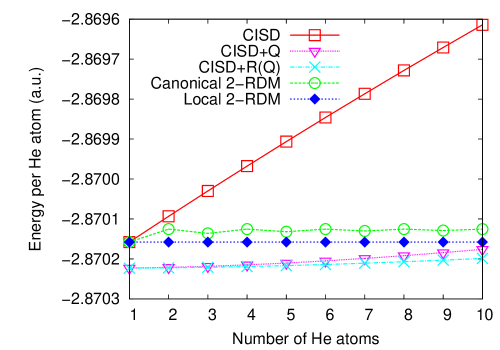
Figure 4: Energy per helium atom as a function of the number of He atoms for a system of non-interacting helium atoms. The 2-RDM method is numerically size-extensive utilizing both canonical and localized molecular orbitals. Size-extensivity is absolutely rigorous in the local orbital basis.

We treat an increasing number of helium atoms at effectively infinite separation to illustrate the size-extensivity of the 2-RDM method in a basis of canonical and localized orbitals. The He atoms are situated on a line with an interatomic distance of 200 Å; the atomic orbitals are represented by an Ahlrichs double-zeta basis set REF:7_ADZ . For the localized-orbital calculations, occupied and virtual orbitals were localized separately according to the Boys localization criterion REF:7_Boys . The energy per He atom for a size-extensive method should not vary with the number of He atoms. We see that the 2-RDM does display this characteristic when utilizing either localized and delocalized canonical orbitals; regardless of the “bumps” in the canonical basis, the 2-RDM results do not display any systematic dependence upon system size. The energies obtained in the local basis, however, are rigorously size-extensive, with no numerical deviation in the energy per He atom for all system sizes. We have also presented the energies obtained from the Davidson correction REF:7_Davidson , denoted CISD+Q, and the renormalized Davidson correction REF:7_RD1 ; REF:7_RD2 , denoted CISD+R(Q). Clearly, neither the Davidson corrected nor renormalized Davidson corrected energies are rigorously size-extensive, with both results exhibiting a clear and systematic dependence on system size.

These results unfortunately demonstrate that the 2-RDM energy is not strictly invariant to unitary transformations among the occupied orbitals, as is the case with traditional CEPA methodologies. Perhaps even more unfortunately, this dependence also extends to the virtual space. The dependence upon the choice of the virtual orbitals is a consequence of the symmetry properties of the topological factor in the occupied and virtual spaces; EPV diagrams are removed from not only the occupied space, as is the case in CEPA, but from the virtual space as well. Figure 5 illustrates the deviation of the energy obtained from calculations with localized orbitals from those performed using canonical Hartree-Fock orbitals for the H-F bond stretch in (a) cc-pVDZ and (b) cc-pVTZ basis sets.

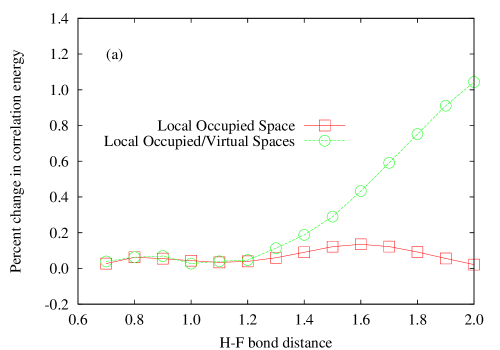
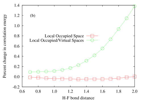
Figure 5: The percentage change in the correlation energy, $\frac{E_{c,\rm{canon}}-E_{c,\rm{local}}}{E_{c,\rm{canon}}}\times 100\%$ when utilizing localized molecular orbitals rather than canonical Hartree-Fock orbitals for the H-F bond stretch in (a) cc-pVDZ and (b) cc-pVTZ basis sets.

We present results for two cases within each basis set: (i) calculations in which only the occupied orbitals are localized and (ii) calculations in which we localize both the occupied and virtual orbitals separately. Clearly, the 2-RDM method is not invariant to unitary transformations in either the occupied or virtual subspaces. Importantly, the method’s variance with respect to the occupied space is nearly constant at all bond lengths and across basis sets. We note that the sign of the percent change for local occupied orbitals changes between basis sets, meaning that the energy with localized orbitals was lower than the canonical case in the cc-pVDZ basis but higher in the cc-pVTZ basis. While the relative magnitudes of the changes are very similar, the change in sign implies that we cannot assume a systematic change in energy for arbitrary systems and basis sets when utilizing localized versus delocalized canonical orbitals. The variance with respect to the virtual space, while being fairly uniform across basis sets, is highly dependent upon the geometry of the system. Local virtual orbitals are in general very difficult to determine; minima are often local in nature in the localization function, and the orbitals themselves may not vary smoothly with nuclear coordinates. It is unclear whether the strong dependence of the energy on the virtual space is a consequence of these difficulties or some other systematic deficiency inherent to the p-2RDM^′/$n$ methods.

We further investigate the dependence of the 2-RDM energy with respect to variations in the virtual space with a size-extensivity example similar to the infinitely separated two-electron systems treated above; we here investigate the size-extensivity of the 2-RDM method of infinitely separated two-hole systems. As in the He example above, a size-extensive double-excitation theory should yield the exact result regardless of system size. Figure 6

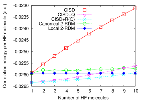
Figure 6: Energy per HF molecule as a function of the number of HF molecule for a system of non-interacting HF molecules. The 2-RDM method is only rigorously size-extensive when using a basis of localize occupied and virtual molecular orbitals.

illustrates the correlation energy for a system of non-interacting HF molecules in a minimal STO-6G basis set. The molecules lie parallel to one another in a line with a distance between each center of mass of 1000 Å. The H-F bond length is taken as the experimentally determined value given in the computational chemistry comparison and benchmark database (CCCBD) REF:7_CCCBD . The 2-RDM method is utilized with either canonical or separately localized occupied and virtual orbitals. As expected, CISD is not size-extensive. The 2-RDM method yields effectively size-extensive results for both choices of orbitals, but the only exactly size-extensive choice is that in which both the local and virtual orbital spaces are localized. Both the Davidson and renormalized Davidson-corrected energies exhibit a strong dependence on system size and are thus not rigorously size-extensive.

IV Conclusions

Parametric variational $2$-RDM methods are an accurate and efficient alternative to traditional ab initio methods. They formally scale the same as CI with single and double excitations and may be implemented at a cost that is slightly less than coupled cluster with single and double substitutions. Provided calculations are performed in a local orbital basis, the obtained energies are rigorously size-extensive. The methods have been previously been generalized for geometry optimizations, harmonic frequency analysis, the treatment of open-shell systems, and local correlation approximations with much success. Novel parametrizations, unique from that originally proposed by Kollmar or discussed in this paper have been presented that result in accuracies similar CCSD(T).

The parametric 2-RDM approach represents a fairly young class of methods, and as such its relationship to other methods has remained to this point unexplored. For this reason, we have drawn connections between parametric 2-RDM methodologies and existing coupled electron pair approximation (CEPA) theories. We have derived a set of topological factors that correspond to the CEPA/$n$ ($n=1,2,3$) family, and the resulting class of methods is a density-based generalization of CEPA/$n$ called p-2RDM/$n$. Extensive numerical studies of equilibrium energies, geometries, and harmonic frequencies have shown that the p-2RDM methods perform very similarly to their CEPA analogues for a variety of closed-shell systems. New topological factors have been derived specifically to account for the exclusion-principle-violating (EPV) terms that arise in the virtual space that are ignored by standard CEPA methodologies. Malrieu and coworkers REF:7_CEPA9 understood the importance of the balance between occupied and virtual EPV diagrams in their self-consistent, size-consistent truncated CI ( (SC)²-CISD ); their proposed method is most similar in spirit to the p-2RDM^′/$3$ variant discussed herein. Another factor, denoted p-2RDM^′/1, is in fact identical to that proposed by Kollmar REF:7_Kollmar . The proper treatment of the virtual space EPV diagrams is necessary in some situations to obtain physically meaningful results, as was demonstrated for the potential energy surface for the CH radical. Consideration of the virtual space EPV diagrams for the p-2RDM/3 method is necessary to avoid an unphysical hump in the dissociation curve. Aside from these numerical arguments, properly treating virtual space EPV diagrams is absolutely essential from the standpoint of density matrix theory in that they are required for a balanced treatment of particles and holes. The parametric 2-RDM framework for p-2RDM is also quite convenient as compared to the standard overlap equation formulation of traditional CEPA methodologies; the energies obtained from any of the p-2RDM or p-2RDM^′ variants presented herein are stationary points, facilitating the evaluation of geometric derivatives and the direct computation of density matrices and their associated one- and two-electron properties.

We have discussed in detail the orbital invariance properties of the CEPA and p-2RDM methods citing various numerical examples. The 2-RDM method is indeed exactly size-extensive, but this claim holds true only under the condition that one utilizes a basis of localized molecular orbitals. As such, the 2-RDM method (and thus the p-2RDM and p-2RMD^′ variants) are not rigorously invariant to unitary transformations within orbital subspaces. The p-2RDM methods display a dependence on the choice of orbitals for the occupied space while the p-2RMD^′ methods also vary with the choice of the virtual orbitals. One may circumvent any ambiguities with respect to the definition of the orbital space by always utilizing a basis of local orbitals. Determining these orbitals in the occupied subspace is trivial by the Boys localization criterion REF:7_Boys , but may prove problematic for the virtual space where local orbitals may not be unique and do not necessarily vary smoothly with nuclear coordinates. Fortunately, the variance in the correlation energy with the occupied orbitals is only a fraction of a percent and at worst on the order of one percent for the virtual orbitals. These discrepancies are very small when compared to the percentage of correlation energy that is not recovered for any of the standard ab initio methods with respect to the exact full CI results.

- (1) A. J. Coleman and V. I. Yukalov, Reduced Density Matrices: Coulson’s Challenge (Springer-Verlag, New York, 2000).
- (2) D. A. Mazziotti (Ed.), Reduced-Density-Matrix Mechanics: With Application to Many-electron Atoms and Molecules, Advances in Chemical Physics, Vol. 134, (Wiley, New York, 2007).
- (3) A. J. Coleman, Rev. Mod. Phys. 35, 668 (1962).
- (4) C. Garrod and J. Percus, J. Math. Phys. 5, 1756 (1964).
- (5) D. A. Mazziotti, Phys. Rev. Lett. 93, 213001 (2004).
- (6) D. A. Mazziotti, J. Chem. Phys. 121, 10957 (2004).
- (7) D. A. Mazziotti, Phys. Rev. A 74, 032501 (2006).
- (8) D. A. Mazziotti, Acc. Chem. Res. 39, 207 (2006).
- (9) G. Gidofalvi and D. A. Mazziotti, J. Chem. Phys. 126, 024105 (2007).
- (10) Z. Zhao, B. J. Braams, H. Fukuda, M. L. Overton, and J. K. Percus, J. Chem. Phys 120, 2095 (2004).
- (11) E. Cancs, G. Stoltz, and M. J. Lewin, J. Chem. Phys. 125, 064101 (2006).
- (12) D. A. Mazziotti, Phys. Rev. Lett. 97, 143002 (2006).
- (13) D. A. Mazziotti, Phys. Rev. A 75, 022505 (2007).
- (14) D. A. Mazziotti, J. Phys. Chem. A 111, 12635 (2007).
- (15) D. A. Mazziotti, J. Chem. Phys. 126, 184101 (2007).
- (16) D. A. Mazziotti, Phys. Rev. A 76, 052502 (2007).
- (17) D. A. Mazziotti, J. Phys. Chem. A 112, 13684 (2008).
- (18) C. Valdemoro, L. M. Tel, D. R. Alcoba, and E. Prez-Romero, Theor. Chem. Acc. 118, 503 (2007).
- (19) C. Valdemoro, L. M. Tel, E. E. Prez-Romero, and D. R. Alcoba, Int. J. Quantum Chem. 108, 1090 (2008).
- (20) D. A. Mazziotti, Phys. Rev. A 57, 4219 (1998).
- (21) F. Colmenero and C. Valdemoro, Phys. Rev. A 47, 979 (1993).
- (22) H. Nakatsuji and K. Yasuda, Phys. Rev. Lett. 76, 1039 (1996).
- (23) C. Kollmar, J. Chem. Phys. 125, 084108 (2006).
- (24) A. E. DePrince III and D. A. Mazziotti, Phys. Rev. A 73, 042501 (2007).
- (25) A. E. DePrince III, E. Kamarchik, and D.A. Mazziotti, J. Chem. Phys. 128, 234103 (2008).
- (26) A. E. DePrince III and D. A. Mazziotti, J. Phys. Chem. B 112, 16158 (2008).
- (27) D. A. Mazziotti, Phys. Rev. Lett. 101, 253002 (2008); Phys. Rev. A 81, 062515 (2010).
- (28) A. E. DePrince III and D. A. Mazziotti, J. Chem. Phys. 130, 164109 (2009).
- (29) A. E. DePrince III and D. A. Mazziotti, J. Chem. Phys. 132, 034110 (2010).
- (30) A. E. DePrince III and D. A. Mazziotti, J. Chem. Phys. 133, 034112 (2010).
- (31) S. Koch and W. Kutzelnigg, Theoret. Chim. Acta 59, 387 (1981).
- (32) R. Ahlrichs, Comput. Phys. Comm. 17, 31 (1979).
- (33) W. Meyer, Int. J. Quant. Chem. 5, 341 (1971).
- (34) W. Meyer, J. Chem. Phys. 58, 1017 (1973).
- (35) P. Taylor, G. B. Bacskay, and N. S. Hush, Chem. Phys. Lett. 41, 444 (1976).
- (36) R. Ahlrichs, P. Scharf, and C. Ehrhardt, J. Chem. Phys. 82, 890 (1985).
- (37) R. J. Gdanitz and R. Ahlrichs, Chem. Phys. Lett. 143, 413 (1988).
- (38) F. Wennmohs, F. Neese, Chem. Phys. 343, 217 (2008).
- (39) M. Nooijen and R. J. Le Roy, J. Molec. Struct.: THEOCHEM 768, 25 (2006).
- (40) F. Neese, A. Hansen, F. Wennmohs, and S. Grimme, Acc. Chem. Res. 42, 641 (2009).
- (41) J.-P. Daudey, J.-L. Heully, and J.-P. Malrieu, J. Chem. Phys. 99, 1240 (1993).
- (42) A. E. DePrince III, A Parametric Approach to Variational Two-electron Reduced Density Matrix Theory, Ph.D. thesis, Department of Chemistry, The University of Chicago, 2009.
- (43) C. Kollmar and F. Neese, Mol. Phys. (2010), DOI: 10.1080/00268976.2010.496743.
- (44) J.-P. Malrieu,H. Zhang, and J. Ma, Chem. Phys. Lett. In Press, Corrected Proof (2010).
- (45) C. Kollmar and A. Heelmann, Theor. Chem. Acc. (in press 2010).
- (46) MOLPRO, version 2006.1, a package of ab initio programs, designed by H.-J. Werner, P. J. Knowles, R. Lindh, F. R. Manby, M. Schütz et al. (see http://www.molpro.net).
- (47) T. D. Crawford, C. D. Sherrill, E. F. Valeev et al., J. Comput. Chem. 28, 1610 (2007).
- (48) M. W. Schmidt, K. K. Baldridge, J. A. Boatz, S. T. Elbert, M. S. Gordon, J. H. Jensen, S. Koseki, N. Matsunaga, K. A. Nguyen, S. Su, T. L. Windus, M. Dupuis, and J. A. Montgomery Jr, J. Comput. Chem. 14, 1347 (1993).
- (49) G. D. Purvis and R. J. Bartlett, J. Chem. Phys. 68, 2114 (1978).
- (50) A. Schafer, H. Horn, and R. Ahlrichs, J. Chem. Phys. 97, 2571 (1992).
- (51) S. F. Boys, Rev. Mod. Phys. 32 296 (1960).
- (52) S. R. Langhoff and E. R. Davidson, Int. J. Quant. Chem. 8, 61 (1974).
- (53) E. M. Siegbahn, Chem. Phys. Lett. 55, 386 (1978).
- (54) L. Meissner, Chem. Phys. Lett. 146, 204 (1988).
- (55) Computational Chemistry Comparison and Benchmark Database, http://srdata.nist.gov/cccbdb