Optimal 3D Angular Resolution for Low-Degree Graphs

Abstract

We show that every graph of maximum degree three can be drawn in three dimensions with at most two bends per edge, and with $120^{\circ}$ angles between any two edge segments meeting at a vertex or a bend. We show that every graph of maximum degree four can be drawn in three dimensions with at most three bends per edge, and with $109.5^{\circ}$ angles, i. e., the angular resolution of the diamond lattice, between any two edge segments meeting at a vertex or bend.

1 Introduction

Much past research in graph drawing has shown the importance of avoiding sharp angles at vertices, bends, and crossings of a drawing, as they make the edges difficult to follow [15]. There has been much interest in finding drawings where the angles at these features are restricted, either by requiring all angles to be at most $90^{\circ}$ (as in orthogonal drawings [11] and RAC drawings [1, 7, 8]) or more generally by attempting to optimize the angular resolution of a drawing, the minimum angle that can be found within the drawing [4, 13, 14, 16].

Three-dimensional graph drawing opens new frontiers for angular resolution in two ways. First, in three-dimensional graph drawing, there is no need for crossings, as any graph can be drawn without crossings; however, finding a compact layout that uses few bends and avoids crossings can sometimes be challenging. Second, and more importantly, in 3d there is a much greater variety in the set of ways that a collection of edges can meet at a vertex to achieve good angular resolution, and the angular resolution that may be obtained in 3d is often better than that for a two-dimensional drawing. For instance, in 3d, six edges may meet at a vertex forming angles of at most $90^{\circ}$, whereas in 2d the same six edges would have an angular resolution of $60^{\circ}$ at best.

The problem of optimizing the angular resolution of a collection of edges incident to a single vertex in 3d is equivalent to the well-known Tammes’ problem of placing points on a sphere to maximize their minimum separation; this problem is named after botanist P. M. L. Tammes who studied it in the context of pores on grains of pollen [18], and much is known about it [5]. For graphs of degree five or six, the optimal angular resolution of a three-dimensional drawing is $90^{\circ}$, as above, achieved by placing vertices on a grid and drawing all edges as grid-aligned polylines. The simplicity of this case has freed researchers to look for three-dimensional orthogonal drawings that, as well as optimizing the angular resolution, also optimize secondary criteria such as the number of bends per edge, the volume of the drawing, or combinations of both [3, 10, 19]. Thus, in this case, it is known that the graph may be drawn with at most 3 bends per edge in an $O(n)\times O(n)\times O(n)$ grid and with $O(1)$ bends per edge in an $O(\sqrt{n})\times O(\sqrt{n})\times O(\sqrt{n})$ grid [10]. For graphs of maximum degree five a tighter bound of two bends per edge is also known [19]; a well known open problem asks whether the same two-bend-per-edge bound may be achieved for degree six graphs [6].

In two dimensions, $90^{\circ}$ angular resolution is optimal for graphs that may be nonplanar, because every crossing has an angle at least this sharp. However, in 3d, crossings are no longer a concern and graphs of degree three and four may have angular resolution even better than $90^{\circ}$. In particular, in the diamond lattice, a subset of the integer grid, the edges are parallel to the long diagonals of the grid cubes and meet at angles of $\arccos(-1/3)\approx 109.5^{\circ}$, the optimal angular resolution for degree-four graphs (Figure 1, left). For graphs with maximum degree three, the best possible angular resolution at any vertex is clearly $120^{\circ}$; three edges with these angles are coplanar, but the planes of the edges at adjacent vertices may differ: for instance, Figure 1(right) shows an infinite space-filling graph in which all vertices are on integer grid points, all edges form face diagonals of the integer grid, and all vertices have $120^{\circ}$ angular resolution.

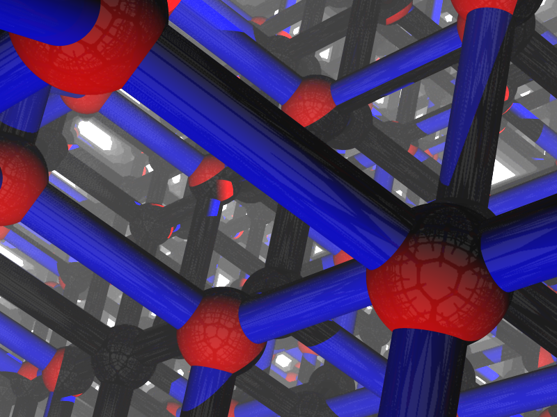
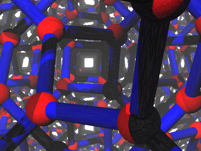
Figure 1: Left: The three-dimensional diamond lattice, from [12]. Right: A space-filling 3-regular graph with $120^{\circ}$ angular resolution.

The primary questions we study in this paper are how to achieve optimal $120^{\circ}$ angular resolution for 3d drawings of arbitrary graphs with maximum degree three, and optimal $109.5^{\circ}$ angular resolution for 3d drawings of arbitrary graphs with maximum degree four. We define angular resolution to be the minimum angle at any bend or vertex, matching the orthogonal drawing case, and we do not allow edges to cross. These questions are not difficult to solve without further restrictions (just place the vertices arbitrarily and use polylines with many bends to connect the endpoints of each edge) so we further investigate drawings that minimize the number of bends, align the vertices and edges of the drawing with the integer grid similarly to the alignment of the spacefilling patterns in Figure 1, and use a small total volume. We show:

• Any graph of maximum degree four can be drawn in 3d with optimal $109.5^{\circ}$ angular resolution with at most three bends per edge, with all vertices placed on an $O(n)\times O(n)\times O(n)$ grid and with all edges parallel to the long diagonals of the grid cubes.

• Any graph of maximum degree three can be drawn in 3d with optimal $120^{\circ}$ angular resolution with at most two bends per edge. However, our technique for achieving this small number of bends does not use a grid placement and does not achieve good volume bounds.

• Any graph of maximum degree three has a drawing with $120^{\circ}$ angular resolution, integer vertex coordinates, edges parallel to the face diagonals of the integer grid, at most three bends per edge, and polynomial volume.

We believe that, as in the orthogonal case, it should be possible to achieve tighter bounds on the volume of the drawing at the expense of greater numbers of bends per edge.

2 Three-bend drawings of degree-four graphs on a grid

Our technique for three-dimensional drawings of degree-four graphs with angular resolution $109.5^{\circ}$ and three bends per edge is based on lifting two-dimensional drawings of the same graphs, with angular resolution $90^{\circ}$ and two bends per edge. The three-dimensional vertex placements are all on the plane $z=0$, essentially unchanged from their two-dimensional placements, but the edges are raised and lowered above and below the plane to avoid crossings and improve the angular resolution.

Our two-dimensional orthogonal drawing technique uses ideas from previous work on drawing degree-four graphs with bounded geometric thickness [9]. We begin by augmenting the graph with dummy edges and a constant number of dummy vertices if necessary to make it a simple 4-regular graph, find an Euler tour in the augmented graph, and color the edges alternately red and green in their order along this path. In this way, the red edges and the green edges each form 2-regular subgraphs [17] consisting of disjoint unions of cycles. We denote the number of red (green) cycles by $m_{\text{red}}$ ($m_{\text{green}}$).

Next, we draw the red subgraph so that every cycle passes horizontally through its vertices with two bends per edge, and we draw the green subgraph so that every cycle passes vertically through its vertices with two bends per edge. We can do that by using the cycle ordering within each of these two subgraphs as one of the two Cartesian coordinates for each point. More precisely, we do the following.

We define the green order of the vertices of the graph to be an order of the vertices such that the vertices of each green path or cycle are consecutive; we define the red order the same way. Let $r_{\text{green}}(v)\geq 0$ be the rank of a vertex $v$ in some green order, and $r_{\text{red}}(v)$ be its rank in some red order. We further order the red and green cycles and define $c_{\text{red}}(v)\geq 0$ and $c_{\text{green}}(v)\geq 0$ to be the ranks in the two cycle orders of the red and green cycles to which $v$ belongs. We embed the vertices on a $(2n+2m_{\text{green}}-4)\times(2n+2m_{\text{red}}-4)$ grid such that the $x$-coordinate of each vertex is $2r_{\text{green}}(v)+2c_{\text{green}}(v)$, and its $y$-coordinate is $2r_{\text{red}}(v)+2c_{\text{red}}(v)$.

Let $v_{1},...v_{k}$ be the vertices of a green cycle $C$ in the green order. We embed $C$ as follows. We mark each end of each edge with a plus or a minus such that at every vertex exactly one end is marked with a plus and exactly one with a minus. We then would like to embed $C$ in such a way that plus would correspond to the edge entering the vertex from above and a minus corresponds to the edge entering the vertex from below. Note that every edge whose two ends are marked the same can be embedded in this way with two bends. Whenever the marks alternate along the edge one can only embed it with two bends if the lower end (the end incident to a vertex with smaller $y$-coordinate) is marked with plus.

We next describe how to label $C$ so that it has a 2-bends-per-edge embedding respecting the labeling. If $k$ is even, we mark both ends of the edge $(v_{1},v_{2})$ with pluses. If $k$ is odd, we mark the higher end of $(v_{1},v_{2})$ with a minus and its lower end with a plus. In both cases there is a unique way to label the rest of the edges such that both ends of each edge have the same signs and the labels alternate at every vertex.

To complete our 2d embedding we draw all edges consistently with the labeling as follows. Each edge $(v_{i},v_{i+1})$ is placed such that the $y$-distance of its horizontal segment to one of the vertices is 1. If the last edge $(v_{1},v_{k})$ is labeled negatively, its horizontal segment is drawn on the grid line one unit below the lowest vertex or bend of $C$. Similarly, if $(v_{1},v_{k})$ is labeled positively, the horizontal segment is drawn one unit above the highest part of $C$. See Figure 2 for an illustration.

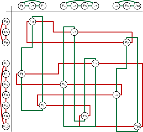
Figure 2: A 4-regular graph with 10 vertices embedded according to the decomposition into disjoint red and green cycles.

Lemma 1

The embedding described above has the following properties:

• no two edges of the same color intersect;

• a vertex lies on an edge if and only if it is incident to the edge;

• no midpoint of an edge coincides with a bend of the edge;

• the embedding fits on a $(2n+2m_{\text{green}})\times(2n+2m_{\text{red}})$ grid.

Proof

Green edges connecting consecutive vertices in the green order of the same cycle $C$ are trivially disjoint. The horizontal segment of the edge connecting the first and the last vertex of $C$ is placed below or above all other edges of $C$. Two different green components are disjoint because the edges of every component are contained inside the vertical strip defined by its first and last vertices and components are ordered along the $x$-axis. The argument for red edges is symmetric.

Since all the vertices have distinct $x$-coordinates, and every green vertical segment has a vertex at one of its ends we can conclude that every vertex is incident to at most two vertical green segments. Every green horizontal segment has odd $y$-coordinate and every vertex has even $y$-coordinate hence a green horizontal segment cannot contain a vertex. The argument for red edges is symmetric.

For arbitrary red and green vertex orders it is possible that the midpoint of an edge coincides with one of its bends. We show that there are red and green vertex orders for which this is not the case. For any edge whose ends are labeled differently we can always place the horizontal segment such that the midpoint of the edge does not coincide with a bend. For edges whose ends have the same label it is easy to see that the midpoint coincides with a bend if and only if the vertical distance and the horizontal distance of its vertices are equal. Apart from the last edge in each green cycle the horizontal distance between any two adjacent vertices $v_{i}$ and $v_{i+1}$ is 2. We claim that the vertical distance between $v_{i}$ and $v_{i+1}$ is larger than 2 since otherwise $v_{i}$ and $v_{i+1}$ are adjacent in a red cycle which contradicts the assumption that the 4-regular graph is simple. Note that this is the reason why different components are spaced by at least 4 units. Finally consider the last edge $(v_{1},v_{k})$ of a cycle $C$ with vertices $v_{1},\dots,v_{k}$. The horizontal distance of $v_{1}$ and $v_{k}$ is $2k-2$. If their vertical distance equals $2k-2$ as well, we cyclically shift the green order of the vertices in $C$ by moving $v_{k}$ to the vertical grid line of $v_{1}$ and shifting each of $v_{1},\dots,v_{k-1}$ two units to the right. Now $(v_{k},v_{k-1})$ is the last edge of $C$. We perform this shifting until the vertices of the last edge no longer have vertical distance $2k-2$. Since every vertex has an exclusive $y$-coordinate there is at least one edge with this property in $C$. The local shifting of $C$ does not influence other parts of the drawing. The argument for red cycles is analogous.

The vertices lie on $(2n+2m_{\text{green}}-4)\times(2n+2m_{\text{red}}-4)$ grid, and each grid line with coordinate $2k$ contains exactly one vertex. The lowest vertex is incident to a green edge with a horizontal segment at the height $-1$; the highest one is incident to a green edge with a horizontal segment at the height $2n+2m_{\text{red}}-3$. One of the green edges connecting the first and last vertices of some cycle can lie one grid line below the height $-1$ or one grid lines above $2n+2m_{\text{red}}-3$.

It remains to lift the 2d drawing described above into three dimensions. We first rotate the drawing by $45^{\circ}$; this expands the grid size to $(4n+4m_{\text{green}})\times(4n+4m_{\text{red}})$. The vertices themselves stay in the plane $z=0$, but we replace each edge by a path in 3d that goes below the plane for the red edges and above the plane for the green edges, eliminating all crossings between red and green edges. The path for a green edge goes upwards along the long diagonals of the diamond lattice cubes until its midpoint, where it has a bend and turns downwards again. The lifted images of the two bends in the underlying 2d edge remain bends in the 3d path and hence we get three bends per edge in total. The red edges are drawn analogously below the plane $z=0$. Since in the original 2d drawing every edge has even length, the midpoint of every edge is a grid point and hence the lifted midpoint is also a grid point of the diamond lattice. By Lemma 1 a midpoint of an edge never coincides with a 2d bend and hence all bend angles as well as the vertex angles are $109.5^{\circ}$ diamond lattice angles. Finally, we remove all the edges we added to make the graph 4-regular. Considering the longest possible red and green edges the total grid size is at most $(4n+4m_{\text{green}})\times(4n+4m_{\text{red}})\times(12n+6m_{\text{green}}+6m_{\text{red}})$. We note that $m_{\text{green}}$, $m_{\text{red}}\leq n/3$ since every component is a cycle. This yields the following theorem.

Theorem 2.1

Any graph $G$ with maximum vertex degree four can be drawn in a 3d grid of size $16n/3\times 16n/3\times 16n$ with angular resolution $109.5^{\circ}$, three bends per edge and no edge crossings.

3 Two-bend drawings of degree-three graphs

The main idea of our algorithm for drawing degree-three graphs with optimal angular resolution and at most two bends per edge is to decompose the graph into a collection of vertex-disjoint cycles. Each cycle of length four or more can be drawn in such a way that the edges incident to the cycle all attach to it via segments that are parallel to the $z$ axis (Lemma 4). By placing the cycles far enough apart in the $z$ direction, these segments can be connected to each other with at most two bends per edge. However, several issues complicate this method:

• Cycles of length three cannot be drawn in the same way, and must be handled differently (Lemma 2).

• Our method for eliminating cycles of length three does not apply to the graph $K_{4}$, for which we need a special-case drawing (Lemma 3).

• Although Petersen’s theorem [2, 17] can be used to decompose any bridgeless cubic graph into cycles and a matching, it is not suitable for our application because some of the matching edges may connect two vertices in a single cycle, a case that our method cannot handle. In addition, we wish to handle graphs that may contain bridges. Therefore, we need to devise a different decomposition algorithm. However, with our decomposition, the complement of the cycles is a forest rather than just a matching, and again we need additional analysis to handle this case.

Figure 3: $\Delta$–Y transformation of a graph $G$ containing a triangle, and undoing the transformation to find a drawing of $G$ (Lemma 2). Top: the contracted vertex has degree three, and is replaced by a hexagon. Bottom: the contracted vertex has degree two, and is replaced by a heptagon.

Lemma 2

Let $G$ be a graph with maximum degree three containing a triangle $uvw$. If $uvw$ is not part of any other triangle, let $G^{\prime}$ be the result of contracting $uvw$ into a single vertex (that is, performing a $\Delta$–Y transformation on $G$). Otherwise, if there is a triangle $vwx$, let $G^{\prime}$ be the result of contracting $uvwx$ into a single vertex. If $G^{\prime}$ can be drawn in 3d with two bends per edge and with angles of at least $120^{\circ}$ between the edges at each vertex or bend, then so can $G$.

Proof

First we consider the case that $G^{\prime}$ is obtained by collapsing $uvw$. The edges incident to the merged vertex $uvw$ must lie in a plane in any drawing of $G^{\prime}$. If $uvw$ has degree zero, one, or three in $G^{\prime}$, or if it has degree two and is drawn with angular resolution exactly $120^{\circ}$, then we may draw $G$ by replacing $uvw$ by a small regular hexagon in the same plane, with at most one bend for each of the three triangle edges (Figure 3, top). If the merged vertex $uvw$ has degree two in $G^{\prime}$ and is drawn with angular resolution greater than $120^{\circ}$, we may replace it by a small heptagon (Figure 3, bottom).

The case that $G^{\prime}$ is obtained by collapsing four vertices $uvwx$ is similar: the collapsed vertex may be replaced by a pair of regular hexagons or irregular heptagons, meeting edge-to-edge. The four vertices $uvwx$ are placed at the points where these two polygons meet the other edges of the drawing and the two endpoints of the edge where they meet each other; the edge $vw$ has no bends and the other edges all have one or two bends.

Lemma 3

The graph $K_{4}$ may be drawn in 3d with all vertices on integer grid points, angular resolution $120^{\circ}$, and at most two bends per edge.

Proof

See Figure 4.

Figure 4: A two-bend drawing of $K_{4}$ with $120^{\circ}$ angular resolution (left) and its two-dimensional projection (right).

Lemma 4

Let $G$ be a graph with maximum degree three, consisting of a cycle $C$ of $n\geq 4$ vertices together with some number of degree-one vertices that are adjacent to some of the vertices in $C$. Suppose also that each degree-one vertex in $G$ is labeled with the number $+1$ or $-1$. Then, there is a drawing of $G$ with the following properties:

• All vertices and bends have angular resolution at least $120^{\circ}$.

• All edges of $C$ have at most two bends.

• All edges attaching the degree-one vertices to $C$ have no bends.

• Every degree-one vertex has the same $x$ and $y$ coordinates as its (unique) neighbor, and its $z$ coordinate differs from its neighbor’s $z$ coordinate by its label. Thus, all edges connecting degree-one vertices to $C$ are parallel to the $z$ axis, all positively labeled vertices are above (in the positive $z$ direction from) their neighbors, and all negatively labeled vertices are below their neighbors.

• No three vertices of $C$ project to collinear points in the $(x,y)$-plane.

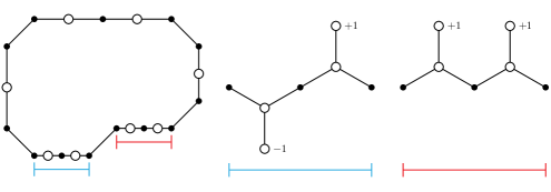
Figure 5: The embedding of a cycle with degree-one neighboring vertices described by Lemma 4. Left: the $xy$-projection of the cycle; cycle vertices are indicated as large hollow circles and bends are indicated as small black disks. Right (at a larger scale): the $xz$-projection of the portions of the embedding corresponding to the two horizontal bottom sides of the $xy$-projected polygon.

Proof

As shown in Figure 5, we draw $C$ in such a way that it projects onto a polygon $P$ in the $xy$-plane, with $135^{\circ}$ angles and with sides parallel to the coordinate axes and at $45^{\circ}$ angles to the axes. There are polygons of this type with a number of sides that can be any even number greater than seven; we choose the number of sides of $P$ so that at least one and at most two vertices of $C$ can be assigned to each axis-parallel side of the polygon. (E. g., when $C$ has from four to eight vertices, $P$ can have eight sides, but when $C$ has more vertices $P$ must be more complex.)

We assign the vertices of $C$ consecutively to the axis-parallel sides of $P$, in such a way that at least one vertex of $C$ and at most two vertices are assigned to each axis-parallel side. If one vertex is assigned to a side, it is placed at the midpoint of that side, and if two vertices are assigned to a side of length $\ell$, then they are placed at distances of $\ell/4$ from one endpoint of the side, as measured in the $xy$ plane, with a bend at the midpoint of the side.

In three dimensions, the diagonal sides of $P$ are placed in the plane $z=0$. For any axis-parallel side of $P$ of length $\ell$ containing $k$ vertices of $C$, we place the vertices with no degree-one neighbor or with a positively labeled neighbor at elevation $z=\ell/(2k\sqrt{3})$, and the vertices with a negatively labeled neighbor at elevation $z=-\ell/(2k\sqrt{3})$, so that the portion of $C$ that projects onto a single side of $P$ forms a polygonal curve with angles of exactly $120^{\circ}$. The degree-one neighbors of the vertices in $C$ are then placed above or below them according to their signs.

With this embedding, each vertex of $C$ gets angular resolution exactly $120^{\circ}$. Any two consecutive vertices of $C$ that are assigned to the same side of $P$ are separated either by zero bends (if their neighbors have opposite signs) or a single bend (if their neighbors have the same signs). Two consecutive vertices of $C$ that belong to two different sides of $P$ are separated by two bends at two of the corners of $P$; these bends have angles of $\arccos(-\sqrt{3/8})\approx 127.8^{\circ}$. By adjusting the lengths of the sides of $P$ appropriately, we may ensure that no three vertices of $C$ project to collinear points in the $xy$-plane.

The main idea of our drawing algorithm is to use Lemma 4, and some simpler cases for individual vertices, to repeatedly extend partial drawings of the given graph $G$ until the entire graph is drawn. We define a vertically extensible partial drawing of a set $S$ of vertices of $G$ to be a drawing of the subgraph $G[S]$ induced in $G$ by $S$, with the following properties:

• The drawing of $G[S]$ has angular resolution $120^{\circ}$ or greater and has at most two bends per edge.

• Each vertex in $S$ has at most one neighbor in $G\setminus S$.

• If a vertex $v$ in $S$ has a neighbor $w$ in $G\setminus S$, then $w$ could be placed anywhere along a ray in the positive $z$-direction from $v$, producing a drawing of $G[S\cup\{w\}]$ that remains non-crossing, continues to have angular resolution $120^{\circ}$ or greater, and has no bends on edge $vw$. We call the ray from $v$ the extension ray for edge $vw$.

• No three extension rays are coplanar.

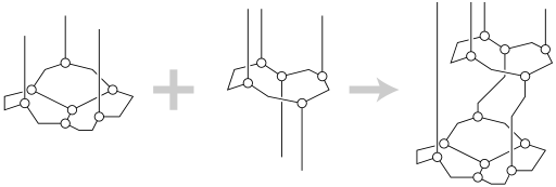
Figure 6: Extending a vertically extensible drawing by adding a cycle.

For instance, if $C$ is a chordless cycle of length four or greater in $G$, then by Lemma 4 there exists a vertically extensible partial drawing of $C$. More, the same lemma may be used to add another cycle to an existing vertically extensible partial drawing (Figure 6):

Lemma 5

For any vertically extensible drawing of a set $S$ of vertices in a graph $G$ of maximum degree three, and any chordless cycle $C$ of length four or more in $G\setminus S$, there exists a vertically extensible drawing of $S\cup C$.

Proof

For each vertex $v$ in $C$ that has a neighbor $w$ in $G$, replace $w$ with a degree-one vertex that has label $-1$ if $w\in S$ and $+1$ if $w\notin S$. Apply Lemma 4 to find a drawing of $C$ that can be connected in the negative $z$-direction to the neighbors of $C$ in $S$, and in the positive $z$-direction for the remaining neighbors of $C$. Translate this drawing of $C$ in the $xy$-plane so that, among the extension rays of $S$ and the vertices of $C$, there are no three points and rays whose projections into the $xy$-plane are collinear and so that, when projected onto the $xy$-plane, the extension rays of $S$ (points in the $xy$-plane) are disjoint from the projection of the drawing of $C$.

For each extension ray of $S$ that connects a vertex $v$ of $S$ to a vertex $w$ in $C$, draw a two-bend path with $120^{\circ}$ bends in the plane containing the extension ray and $w$, such that the final segment of the path has the same $x$ and $y$ coordinates of $w$. By making the transverse section of this path be far enough away from $S$ in the positive $z$ direction, it will not intersect any other features of the existing drawing, and it cannot cross any of the other extension rays due to the requirement that no three of these rays be coplanar. If $C$ is translated in the positive $z$ direction farther than all of the bends in these paths, it can be connected to $S$ to form a vertically extensible drawing of $S\cup C$, as required.

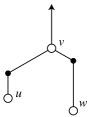
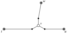
Figure 7: Left: Adding a vertex $v$ with two neighbors $u$ and $w$ in $S$ and one neighbor in $G\setminus S$ to a vertically extensible drawing (shown in the plane of the extension rays of $u$ and $w$). Right: Adding a vertex $v$ with three neighbors $t$, $u$, and $w$ in $S$ (shown in the $xy$-plane). The three segments incident to $v$ are parallel to the $xy$ plane and the three remaining transverse segments form $120^{\circ}$ angles to the extension rays of $t$, $u$, and $w$. The bends where these transverse segments meet their extension rays are shown on top of the three points $t$, $u$, and $w$.

Lemma 6

For any vertically extensible drawing of a set $S$ of vertices in a graph $G$ of maximum degree three, and any vertex $v$ in $G\setminus S$ with at most two neighbors in $S$ and at most one neighbor in $G\setminus S$, there exists a vertically extensible drawing of $S\cup\{v\}$.

Proof

If $v$ has no neighbors in $S$, then $v$ may be placed anywhere on any $z$-parallel line that does not pass through a feature of the existing drawing and is not coplanar with any two existing extension rays. If $v$ has a single neighbor $w$ in $S$, then $v$ may be placed anywhere on the extension ray of $wv$.

In the remaining case, $v$ connects to two extension rays of $S$. Within the plane of these two rays, we may connect $v$ to these two rays by transverse segments at $120^{\circ}$ angles to the rays. By placing $v$ far enough in the positive $z$ direction, these transverse segments can be made to avoid any existing features of the drawing. The extension ray from $v$ can lie on any line parallel to and between the lines of the two incoming extension rays; only finitely many of these lines lead to coplanarities with other extension rays, so it is always possible to place $v$ avoiding any such coplanarity. As shown in Figure 7(left), this construction produces one bend on each edge into $v$.

Lemma 7

If we are given a vertically extensible drawing of a set $S$ of vertices in a graph $G$ of maximum degree three, and a vertex $v$ in $G\setminus S$ that has three neighbors $t$, $u$, and $w$ in $S$, then there exists a vertically extensible drawing of $S\cup\{v\}$.

Proof

Suppose that $tu$ is the longest edge of the triangle formed by the projections of $t$, $u$, and $w$ into the $xy$ plane. Then, as a first approximation to the position of $v$ in the $xy$-plane, let the (two-dimensional) point $v^{\prime}$ be placed on edge $tu$ of this triangle, at the point where $v^{\prime}w$ is perpendicular to $tu$. We adjust this position along edge $tu$, keeping the angle between $v^{\prime}w$ and $tu$ close to $90^{\circ}$ in order to ensure that line segment $v^{\prime}w$ does not pass through the two-dimensional projection of any extension ray. Then, we replace $v^{\prime}$ by three short line segments at $120^{\circ}$ angles to each other meeting the three line segments $v^{\prime}t$, $v^{\prime}u$, and $v^{\prime}w$ at angles of $150^{\circ}$, $150^{\circ}$, and close to $180^{\circ}$. Let $v$ be the point where these three short line segments meet.

This configuration can be lifted into three-dimensional space by placing $v$ and the three edges that attach to it in a plane perpendicular to the $z$ axis, and by replacing the remaining portions of line segments $v^{\prime}t$, $v^{\prime}u$, and $v^{\prime}w$ by transverse segments that make $120^{\circ}$ angles with the extension rays of $t$, $u$, and $w$. There are two bends per edge: one at the point where the extension ray of $t$, $u$, or $w$ meets a transverse segment, and one where a transverse segment meets one of the horizontal segments incident to $v$.

The angles at the bends on the extension rays of $t$, $u$, and $w$ are all exactly $120^{\circ}$, and the angles at the other bends on the paths connecting $t$ and $u$ to $w$ are $\arccos(3/4)\approx 138.6^{\circ}$. As long as segment $v^{\prime}w$ stays within $54^{\circ}$ of perpendicular to $tu$ in the $xy$-plane, the angle at the final remaining bend will be at least $120^{\circ}$.

The construction of Lemma 7 is illustrated in Figure 7(right).

Theorem 3.1

Any graph $G$ of degree three has a drawing with $120^{\circ}$ angular resolution and at most two bends per edge.

Proof

While $G$ contains a triangle, apply Lemma 2 to simplify it, resulting in either $K_{4}$ or a triangle-free graph $G^{\prime}$. If this simplification process leads to $K_{4}$, draw it according to Lemma 3. Otherwise, starting from $S=\emptyset$, we repeatedly grow a vertically extensible drawing of a subset $S$ of $G^{\prime}$ until all of $G^{\prime}$ has been drawn. If $G^{\prime}\setminus S$ contains a vertex with at most one neighbor in $G^{\prime}\setminus S$, then either Lemma 6 or Lemma 7 applies and we can add this vertex to the vertically extensible drawing. Otherwise, all vertices in $G^{\prime}\setminus S$ have two or more neighbors in $G^{\prime}\setminus S$, so $G^{\prime}\setminus S$ contains a cycle. Let $C$ be the shortest cycle in $G^{\prime}\setminus S$; it has length at least four (because we eliminated all triangles) and no chords (because a chord would lead to a shorter cycle) so we may apply Lemma 5 to incorporate it into the vertically extensible drawing. Once we have included all vertices in the vertically extensible drawing, we have drawn all of $G^{\prime}$, and we may reverse the transformations performed according to Lemma 2 to produce a drawing of $G$.

4 Three-bend drawings of degree-three graphs on a grid

In this section we provide an algorithm for embedding a degree-three graph on a grid, using a similar approach to Theorem 3.1 but with up to three instead of two bends per edge. The grid will consist of the face diagonals of the cubes in a regular grid of cubes. First of all, we will make a change of coordinates that allows us an easier description. Define the $xy$-plane to be the plane spanned by the edges $e_{X}=(0,1,1)$ and $e_{Y}=(1,1,0)$ and the $yz$-plane to be the plane spanned by vectors $e_{Y}$ and $e_{Z}=(1,0,1)$. See Figure 8(a).

We will draw the different parts of the drawing in either a horizontal plane (parallel to the $xy$-plane) or in a vertical plane (parallel to the $yz$-plane). The edges we use in the $xy$-plane are parallel to an edge in the set $E_{XY}=\{e_{X},e_{Y},e_{X}-e_{Y}\}$ and they all form angles of $120^{\circ}$. Similarly, in the $yz$-plane, all edges are parallel to an edge in $E_{YZ}=\{e_{Y},e_{Z},e_{Y}-e_{Z}\}$. We will only use integer edge lengths.

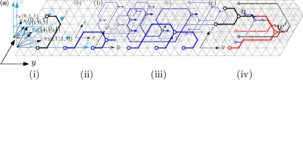
Figure 8: (a) the three base vectors; (b) a cycle in a horizontal plane; (c) the tree structure connecting the extension rays in a set of three neighboring vertical planes (indicated by different colors).

The construction works similarly to the one described in Section 3. In particular, we use exactly the same decomposition of the graph into cycles and trees, and we still draw every cycle in a different horizontal plane and extend the drawing in $z$-direction with every new cycle. However, there are some important differences. First of all, we no longer point the extension rays up (in the $z$-direction), but to the right (the $y$-direction), within the plane in which we draw the cycle. As a result, the drawing of a cycle is completely flat. Then, we draw the trees in vertical planes through the extension rays of the respective vertices. Figure 8(b) and (c) shows the general idea.

Lemma 8

Let $G$ be a graph with maximum degree three, consisting of a cycle $C$ of $n\geq 3$ vertices together with some number of degree-one vertices that are adjacent to some of the vertices in $C$. Let $x_{1},\ldots,x_{n}$ be a set of distinct even integers bounded by $O(n)$. Then, there is a drawing of $G$ in the $xy$-plane with the following properties:

• All vertices and bends have angular resolution $120^{\circ}$.

• All edges of $C$ have at most three bends.

• All edges of $G$ are parallel to an edge in $E_{XY}$.

• For every degree-one vertex $v=(x_{v},y_{v},z_{v})$ and its neighbor $u=(x_{u},y_{u},z_{u})$ we have $x_{v}=x_{u}$, $y_{v}=y_{u}+1$, and $z_{v}=z_{u}$.

• The drawing fits into a grid of size $O(n)\times O(n^{2})$.

• The $x$-coordinate of a vertex $v_{i}$ of $C$ is $x_{i}$, for all $1\leq i\leq n$.

Proof

We embed each cycle in a similar manner as in Section 2. We label each end of each edge of the cycle with a plus or a minus sign such that at every vertex exactly one end is marked with a plus sign and exactly one with a minus sign. We construct this labeling in exactly the same way as in Section 2. Suppose that the $y$-axis of the $xy$-plane points horizontally to the right. We then would like to embed the cycle in the hexagonal grid of the $xy$-plane in such a way that edges labeled with a plus sign enter the vertex from above and edges labeled with a minus sign enter the vertex from below. Moreover, the edge-segment entering a vertex from below is $e_{X}$-parallel and the edge-segment entering a vertex from above is $(e_{X}-e_{Y})$-parallel. With this orientation for the edges, every edge whose ends have identical labels can be embedded with exactly three bends. However, an edge that has opposite signs at its two ends can only be embedded with three bends if its lower end (the end incident to a vertex with smaller $x$-coordinate) is the end labeled with a plus sign. We then embed the edges and vertices as follows.

• We place the vertex $v_{1}$ at some point $(x_{1},y_{1})$ in the $xy$-plane, where $x_{1}$ is its given $x$-coordinate.

• If the cycle contains an odd number of vertices then the first edge $(v_{1},v_{2})$ is labeled with two opposite signs, and is drawn as follows assuming that $v_{1}$ is the lower of the two vertices. From $v_{1}$ we draw an $e_{X}-e_{Y}$-parallel edge segment followed by an $e_{X}$-parallel segment of equal length such that we reach the $e_{Y}$-parallel line at $x=x_{2}$. We place $v_{2}$ at that position.

• If $i>1$ or if $i=1$ and the cycle has an even number of vertices, then edge $v_{i},v_{i+1}$ is labeled with two plus signs or two minus signs. In the case that it is labeled with two plus signs, we start drawing an $e_{X}-e_{Y}$-parallel edge segment from $v_{i}$ followed by an $e_{X}$-parallel segment of equal length until we reach an $e_{Y}$-parallel line that is two units above the higher of the two vertices. If these edge segments intersect any previous part of the drawing we may need to spread the drawing in the $e_{Y}$-direction by a distance of $O(n)$ that is added to the length of an $e_{Y}$-parallel edge. From there we add a unit-length $e_{Y}$-parallel segment and another $e_{X}-e_{Y}$-parallel segment until we reach the $e_{Y}$-parallel line with $x=x_{i+1}$. This is where we place $v_{i+1}$. We proceed symmetrically for any edge marked with two minuses.

• For the edge $(v_{1},v_{n})$ the only difference is that its $e_{Y}$-parallel segment is placed either two units below the lowest point or two units above the highest point of the drawing according to its labels.

Finally, we embed each degree-one vertex one unit to the right of its cycle-neighbor. See Figure 8(b) for an illustration. Note that the size of the grid for drawing $G$ is linear in the $x$-direction but in the worst case quadratic in the $y$-direction.

As in our two-bend non-grid embedding for degree-three graphs, our overall embedding algorithm begins by finding and embedding a chordless cycle of a given graph $G$ and then extends partial drawings of our graph $G$ using Lemma 8 until we obtain the drawing of the entire graph. We define an extensible partial grid-drawing of a set $S$ of vertices of $G$ to be a crossing-free grid-drawing of the subgraph $G[S]$ induced in $G$ by $S$, with the following properties:

• The drawing of $G[S]$ has angular resolution $120^{\circ}$.

• Each vertex in $S$ has at most one neighbor in $G\setminus S$.

• Each vertex in $G\setminus S$ has at most one neighbor in $S$.

• If a vertex $v$ in $S$ has a neighbor $w$ in $G\setminus S$, then we can draw an edge $(v,w)$ with at most three bends of $120^{\circ}$ that starts with an $e_{Y}$-parallel edge segment called the extension ray of $v$. The placement of $(v,w)$ and $w$ is such that the resulting drawing of $G[S\cup\{w\}]$ has angular resolution $120^{\circ}$ and remains extensible and non-crossing.

• For any $x$-coordinate $x_{0}$ there is at most one vertex $v$ in the vertical plane through $x_{0}$ with an active extension ray, i. e., an extension ray that is not yet part of an actual edge $(v,w)$ since $w$ is still a vertex in $G\setminus S$.

• All vertices in $S$ have even $z$-coordinates.

One difference between these properties and the ones used for our two-bend drawings is the requirement that each vertex in $G\setminus S$ have at most one neighbor in $S$. To meet this requirement, when we add a cycle to the drawing, we will also add more vertices until this requirement is met. To formalize this, define the double-adjacency closure of a set of vertices $S$ in a graph $G$ to be the smallest superset $W(S)\supseteq S$ such that every vertex in $G\setminus W(S)$ that is adjacent to $W(S)$ has at least two other neighbors in $G\setminus W(S)$. The double-adjacency closure of $S$ may be obtained by initializing a variable set $W$ to be empty and then repeatedly adding to $W$ any vertex in $G\setminus(S\cup W)$ that has at most one neighbor in $G\setminus(S\cup W)$ until no more such vertices exist; once this process converges, the double-adjacency closure $W(S)$ is $S\cup W$.

Lemma 9

For any extensible grid-drawing of a set $S$ of vertices in a graph $G$ of maximum degree three, and any chordless cycle $C$ in $G\setminus S$, there exists an extensible grid-drawing of $W(S\cup C)$, where $W(S\cup C)$ is the double-adjacency closure of $S\cup C$.

Proof

For each vertex $v$ in $C$ that has a neighbor $w$ in $G$, replace $w$ with a degree-one vertex. We next determine the $x$-coordinate $x_{v}$ for each vertex $v$ of $C$ as follows. If $v$ is adjacent to some vertex $w$ in $S$ or there is a third vertex $u$ in $G\setminus(S\cup C)$ that is adjacent to both $v$ and some vertex $w$ in $S$ then we set $x_{v}$ to be the $x_{w}$ (we can do that because $w$ is unique). The same applies if there is a vertex $u$ in $G\setminus(S\cup C)$ that is adjacent to both $v$ and an already placed vertex $w$ of $C$. Otherwise we set $x_{v}$ to be the smallest even integer which is distinct from $x$-coordinates of all vertices in $S$ and all vertices in $C$ whose $x$-coordinates are already set. There is another special case to deal with: Let $u$ be a degree-three vertex in the double-adjacency closure $W(C)$ that has two neighbors in $W(C)$ and one neighbor $w$ in $S$. Then initially $u$ and all its predecessors in $W(C)$ are assigned a new $x$-coordinate. We need, however, that $u$ and all its predecessors are assigned the $x$-coordinate of $w$.

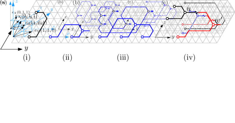
Figure 9: Different cases for connecting $S$ with a new cycle $C$ (from left to right): i) an edge between two different cycles; ii) a vertex connected to two vertices of the same cycle; iii) a vertex connected to three vertices of the same cycle; iv) a vertex $u$ connected to two different cycles and then connected via $w$ to a third cycle involving a switch of vertical planes (indicated by $\sim$).

We will apply Lemma 8 to find a drawing of the double-adjacency closure $W(C)$ with the $x$-coordinates defined above such that $C$ is drawn in a horizontal plane. We place this horizontal plane high enough above the existing drawing of $S$ such that all the connections between $C$ and $S$ can be drawn as 3-bend grid-paths with appropriate angular resolution. Note that since every cycle can spread as much as $O(n^{2})$ in y-direction, we might have to draw the new cycle as far as $O(n^{2})$ away from the existing drawing in z-direction. If there is a vertex $u$ in $W(C)\setminus C$ that is adjacent to two vertices $v,w$ in $C$ then $v$ and $w$ lie in the same vertical plane. We place $u$ in that vertical plane and set its $z$-coordinate to be the next unused even $z$-coordinate above the drawing of $C$. Let $v$ have lower $y$-coordinate than $w$. Then we draw the edge $(v,u)$ in the vertical plane with three bends, where its four segments are $e_{Y}$-parallel, $e_{Z}$-parallel, $e_{Y}$-parallel, and $e_{Y}-e_{Z}$-parallel starting from $v$, see Figure 9(ii). Thus $(v,u)$ connects to $u$ from above. We then draw the edge $(w,u)$ with a single bend connecting to $u$ from below. If required we can place an extension ray for $u$ that is $e_{Y}$-parallel. If there is a vertex $u$ in $W(C)\setminus C$ that is adjacent to three vertices $v,w,t$ in $C$ then by construction all three vertices have the same $x$-coordinate. Let $v,w,t$ be ordered by increasing $y$-coordinate. Then we place $u$ as if it had the two neighbors $v$ and $w$ in $C$. Since $t$ is the rightmost vertex we can connect it with a three-bend edge to the extension ray of $u$ in the vertical plane of $u,v,w,t$, see Figure 9(iii). We note that this drawing of the double-adjacency closure $W(C)$ has indeed at most one active extension ray in each vertical plane.

Now we connect $W(C)$ to $S$. For each vertex $w$ of $S$ that is adjacent to a vertex $v$ in $W(C)$, draw a three-bend grid-path with $120^{\circ}$ bends in the plane containing the extension rays of $v$ and $w$. Since $w$ and $v$ are placed at grid points with the same $x$-coordinates, this plane is parallel to the $yz$-plane and the edge $(v,w)$ follows the grid, see Figure 9(i).

Similarly, if there is a vertex $u$ in $W(S\cup C)$ that is adjacent to a vertex $v$ in $C$ and a vertex $w$ in $S$ we have assigned identical $x$-coordinates to $v$ and $w$ and connect them in a vertical plane with three bends as if there was an edge $(v,w)$. Then, however, we insert the vertex $u$ at the middle bend of the edge, and, if $u$ has degree three, add an $e_{Y}$-parallel extension ray to $u$.

For any vertex $u$ in $W(S\cup C)$ that we introduce we need to check whether $u$ has a common neighbor $w^{\prime}$ in $W(S\cup C)$ together with another vertex $v^{\prime}$ in $S\cup C$. If that is the case we also add $w^{\prime}$ in the vertical plane of $v^{\prime}$ as follows. The $x$-coordinates of $u$ and $v^{\prime}$ do not match. However, since $u$ has an exclusive $z$-coordinate, we can spend two bends in the horizontal plane of $u$ to shift its extension ray to the $x$-coordinate of $v^{\prime}$. Then we add $w^{\prime}$ in the vertical plane of $v^{\prime}$ so that the edge $(u,w^{\prime})$ has three bends and the edge $(v^{\prime},w^{\prime})$ has at most three bends. This is illustrated in Figure 9(iv). We continue this process until all vertices in $W(S\cup C)$ are placed.

Note that we never introduce crossings when drawing edges in vertical planes. As we now show, there is at most one active extension ray in any vertical plane at any time. And since we extend the drawing in the positive $y$-direction this active extension ray is always rightmost in its vertical plane. By construction, this is the case for the existing drawings of $S$ and $W(C)$. Now we consider the combined drawing. It is certainly still true after we assign an unused $x$-coordinate $x_{0}$ to a vertex $v$. We will only assign the $x$-coordinate $x_{0}$ again if a new vertex $w$ connects either directly or via an intermediate vertex $u$ in $W(S\cup C)$ to $v$. In the first case we draw the edge $(v,w)$ and have no more active extension rays. In the second case, we add the vertex $u$, which is then the only vertex with an active extension ray in this plane, and $u$ is to the right of $v$ and $w$. Whenever we use the active extension ray of a vertex $v$ to connect to a new vertex $w$ then the $z$-coordinate of $w$ is larger than the $z$-coordinate of any existing point in that vertical plane. So we connect the rightmost point with the topmost point in the vertical plane, and hence the new edge does not produce crossings.

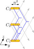
Figure 10: Connections between cycles $C_{i}$ and $C_{j}$ can be forced to immediately move their horizontal planes (because of crossings within that plane), so they have to be spaced enough to make any connection possible. Since one cycle has size $n^{2}$, their spacing is $O(n^{2})$ and the total distance in the $z$-direction is $O(n^{3})$, and the resulting distance in the $y$-direction is therefore also $O(n^{3})$.

The next theorem follows from Lemma 9 and Figure 10.

Theorem 4.1

Any graph $G$ with maximum vertex degree three can be drawn in a 3d grid of size $O(n^{3})\times O(n^{3})\times O(n^{3})$ with angular resolution $120^{\circ}$, three bends per edge and no edge crossings.

Proof

As in our two-bend drawing of the same graphs, we decompose the graph into a sequence of cycles and isolated vertices, where each isolated vertex belongs to the doubly-adjacent closure of the previous cycles. We apply Lemma 9 to extend the drawing for each successive cycle. We start by drawing the first cycle in the $z=0$ plane, and extend the drawing by always adding new cycles above the first one and drawing trees extending into the $y$-direction. Our drawing uses $O(n)$ different $yz$ planes, and therefore has extent $O(n)$ in the $x$ direction of our modified coordinate system. As the analysis in Figure 10 shows, it extends for $O(n^{3})$ units in the other two coordinate directions. This leads to a final drawing of size $O(n)\times O(n^{3})\times O(n^{3})$ in our modified coordinate system.

Finally, if we change the coordinate system back to the more standard Cartesian coordinates, this means that in each dimension the size can be $O(n^{3})$.

5 Conclusions

We have shown how to draw degree-three graphs in three dimensions with optimal angular resolution and two bends per edge, and how to draw degree-four graphs in three dimensions with optimal angular resolution, three bends per edge, integer vertex coordinates, and cubic volume. Multiple questions remain open for investigation, however:

• It does not seem to be possible to draw $K_{4}$ or $K_{5}$ in three dimensions with optimal angular resolution and one bend per edge. Can this be proven rigorously?

• Does every degree-four graph have a drawing in three dimensions with optimal angular resolution and two bends per edge? In particular, is this possible for $K_{5}$?

• How many bends per edge are necessary to draw degree-three graphs with optimal angular resolution in an $O(n)\times O(n)\times O(n)$ grid, with all edges parallel to the face diagonals of the grid?

• It should be possible to draw degree-three and degree-four graphs with optimal angular resolution in an $O(\sqrt{n})\times O(\sqrt{n})\times O(\sqrt{n})$ grid. How many bends per edge are necessary for such a drawing?

Acknowledgments

This research was supported in part by the National Science Foundation under grant 0830403, by the Office of Naval Research under MURI grant N00014-08-1-1015, and by the German Research Foundation (DFG) under grant NO 899/1-1.

References

- [1] P. Angelini, L. Cittadini, G. Di Battista, W. Didimo, F. Frati, M. Kaufmann, and A. Symvonis. On the perspectives opened by right angle crossing drawings. Proc. 17th Int. Symp. Graph Drawing (GD 2009), pp. 21–32. Springer-Verlag, LNCS 5849, 2010, doi:10.1007/978-3-642-11805-0_5.
- [2] T. C. Biedl, P. Bose, E. D. Demaine, and A. Lubiw. Efficient algorithms for Petersen’s matching theorem. Journal of Algorithms 38(1):110–134, 2001, doi:10.1006/jagm.2000.1132.
- [3] T. C. Biedl, T. Thiele, and D. R. Wood. Three-dimensional orthogonal graph drawing with optimal volume. Algorithmica 44(3):233–255, 2006, doi:10.1007/s00453-005-1148-z.
- [4] J. Carlson and D. Eppstein. Trees with convex faces and optimal angles. Proc. 14th Int. Symp. Graph Drawing (GD 2006), pp. 77–88. Springer-Verlag, LNCS 4372, 2007, doi:10.1007/978-3-540-70904-6_9, arXiv:cs.CG/0607113.
- [5] B. W. Clare and D. L. Kepert. The closest packing of equal circles on a sphere. Proc. Roy. Soc. London A 405(1829):329–344, 1986, doi:10.1098/rspa.1986.0056.
- [6] E. D. Demaine. Problem 46: 3D minimum-bend orthogonal graph drawings. The Open Problems Project, 2002, http://maven.smith.edu/~orourke/TOPP/P46.html. Posed by David R. Wood at the CCCG 2002 open-problem session.
- [7] W. Didimo, P. Eades, and G. Liotta. Drawing graphs with right angle crossings. Proc. 11th Int. Symp. Algorithms and Data Structures (WADS 2009), pp. 206–217. Springer-Verlag, LNCS 5664, 2009, doi:10.1007/978-3-642-03367-4_19.
- [8] V. Dujmović, J. Gudmundsson, P. Morin, and T. Wolle. Notes on large angle crossing graphs, arXiv:0908.3545. 2009.
- [9] C. A. Duncan, D. Eppstein, and S. G. Kobourov. The geometric thickness of low degree graphs. Proc. 20th ACM Symp. Computational Geometry (SoCG 2004), pp. 340–346, 2004, doi:10.1145/997817.997868, arXiv:cs.CG/0312056.
- [10] P. Eades, A. Symvonis, and S. Whitesides. Three-dimensional orthogonal graph drawing algorithms. Discrete Applied Mathematics 103(1–3):55–87, 2000, doi:10.1016/S0166-218X(00)00172-4.
- [11] M. Eiglsperger, S. P. Fekete, and G. W. Klau. Orthogonal graph drawing. Drawing Graphs: Methods and Models, pp. 121–171. Springer-Verlag, LNCS 2025, 2001, doi:10.1007/3-540-44969-8_6.
- [12] D. Eppstein. Isometric diamond subgraphs. Proc. 16th Int. Symp. Graph Drawing (GD 2008), pp. 384–389. Springer-Verlag, LNCS 5417, 2009, doi:10.1007/978-3-642-00219-9_37.
- [13] A. Garg and R. Tamassia. Planar drawings and angular resolution: algorithms and bounds. Proc. 2nd Eur. Symp. Algorithms (ESA 1994) (LNCS) 855:12–23, 1994, doi:10.1007/BFb0049393.
- [14] C. Gutwenger and P. Mutzel. Planar polyline drawings with good angular resolution. Proc. 6th Int. Symp. Graph Drawing (GD 1998), pp. 167–182. Springer-Verlag, LNCS 1547, 1998, doi:10.1007/3-540-37623-2_13.
- [15] W. Huang, S.-H. Hong, and P. Eades. Effects of crossing angles. Proc. IEEE Pacific Visualization Symp., pp. 41–46, 2008, doi:10.1109/PACIFICVIS.2008.4475457.
- [16] S. Malitz. On the angular resolution of planar graphs. Proc. 24th ACM Symp. Theory of Computing (STOC 1992), pp. 527–538, 1992, doi:10.1145/129712.129764.
- [17] J. Petersen. Die Theorie der regulären Graphs. Acta Math. 15(1):193–220, 1891, doi:10.1007/BF02392606.
- [18] P. M. L. Tammes. On the origin of the number and arrangement of the places of exit on the surface of pollen grains. Ree. Trav. Bot. Néerl. 27:1–82, 1930.
- [19] D. R. Wood. Optimal three-dimensional orthogonal graph drawing in the general position model. Theoretical Computer Science 299(1-3):151–178, 2003, doi:10.1016/S0304-3975(02)00044-0.