MOIRCS Deep Survey. VIII. Evolution of Star Formation Activity as a Function of Stellar Mass in Galaxies since $z\sim 3$

Abstract

We study the evolution of star formation activity of galaxies at $0.5<z<3.5$ as a function of stellar mass, using very deep NIR data taken with Multi-Object Infrared Camera and Spectrograph (MOIRCS) on the Subaru telescope in the GOODS-North region. The NIR imaging data reach $K\sim$ 23–24 Vega magnitude and they allow us to construct a nearly stellar mass-limited sample down to $\sim 10^{9.5-10}$ M_⊙ even at $z\sim 3$. We estimated star formation rates (SFRs) of the sample with two indicators, namely, the Spitzer/MIPS 24$\mu$m flux and the rest-frame 2800 Å luminosity. The SFR distribution at a fixed M_star shifts to higher values with increasing redshift at $0.5<z<3.5$. More massive galaxies show stronger evolution of SFR at $z\gtrsim 1$. We found galaxies at $2.5<z<3.5$ show a bimodality in their SSFR distribution, which can be divided into two populations by a constant SSFR of $\sim$ 2 Gyr^-1. Galaxies in the low-SSFR group have SSFRs of $\sim$ 0.5–1.0 Gyr^-1, while the high-SSFR population shows $\sim$ 10 Gyr^-1. The cosmic SFRD is dominated by galaxies with M${}_{\rm star}=10^{10-11}$ M_⊙ at $0.5<z<3.5$, while the contribution of massive galaxies with M${}_{\rm star}=10^{11-11.5}$ M_⊙ shows a strong evolution at $z>1$ and becomes significant at $z\sim 3$, especially in the case with the SFR based on MIPS 24 $\mu$m. In galaxies with M${}_{\rm star}=10^{10-11.5}$ M_⊙, those with a relatively narrow range of SSFR ($\lesssim$ 1 dex) dominates the cosmic SFRD at $0.5<z<3.5$. The SSFR of galaxies which dominate the SFRD systematically increases with redshift. At $2.5<z<3.5$, the high-SSFR population, which is relatively small in number, dominates the SFRD. Major star formation in the universe at higher redshift seems to be associated with a more rapid growth of stellar mass of galaxies.

1. Introduction

Determining how galaxies build up their stellar mass is crucial for understanding galaxy formation and evolution. The star formation rate (SFR) and the stellar mass, which is approximately considered as the integral of the past SFR, are the most important physical properties of galaxies to investigate their stellar mass assembly history. Many previous studies measured the comoving cosmic SFR density as a function of redshift, which provides a global picture of star formation history in the universe, using the rest-frame UV luminosity (e.g., Lilly et al., 1996; Madau et al., 1996; Connolly et al., 1997; Madau et al., 1998; Cowie et al., 1999; Steidel et al., 1999; Schiminovich et al., 2005; Bouwens et al., 2007; Reddy et al., 2008), the mid-infrared (MIR) flux (e.g., Le Floc’h et al., 2005; Pérez-González et al., 2005; Babbedge et al., 2006; Caputi et al., 2007; Magnelli et al., 2009), the optical nebular emission lines (Yan et al., 1999; Ly et al., 2007; Geach et al., 2008; Shim et al., 2009; Dale et al., 2010). These studies revealed that the cosmic SFR density increases by an order of magnitude from $z\sim 0$ to $z\sim 1$, and then reaches a peak around $z\sim 2$ and decreases at higher redshift (Hopkins, 2004; Hopkins & Beacom, 2006). On the other hand, recent near-infrared (NIR) surveys enable to measure the average stellar mass density of the universe and several studies based on deep NIR surveys found that a rapid evolution of the cosmic stellar mass density occurred at $1\lesssim z\lesssim 3$ (e.g., Dickinson et al., 2003; Fontana et al., 2006; Kajisawa et al., 2009 and reference therein). These results suggest that a significant fraction of the stellar mass in the present universe had been formed at $z\sim$ 1–3.

The next step to understand how star formation and stellar mass assembly proceeded in galaxies at $1\lesssim z\lesssim 3$ is to investigate the SFR of these galaxies as a function of stellar mass and redshift. Multi-wavelength data from surveys such as COMBO-17, GOODS, COSMOS, UKIDSS, and AEGIS, have been used to measure SFR and stellar mass of galaxies at $1\lesssim z\lesssim 3$ in many studies, where SFRs are estimated from various indicators, namely, the rest-frame UV luminosity (Juneau et al., 2005; Daddi et al., 2007; Feulner et al., 2007; Cowie & Barger, 2008; Drory & Alvarez, 2008; Mobasher et al., 2009; Magdis et al., 2010), the Spitzer/MIPS 24 $\mu$m flux (Papovich et al., 2006; Elbaz et al., 2007; Noeske et al., 2007; Zheng et al., 2007; Santini et al., 2009; Damen et al., 2009a; Damen et al., 2009b), the H$\alpha$ emission line (Erb et al., 2006; Förster Schreiber et al., 2009), and the radio continuum emission (Pannella et al., 2009; Dunne et al., 2009). These studies found that the average SFR or SSFR of star-forming galaxies at a fixed stellar mass increases with redshift strongly. The rate of incline is similar in all stellar mass ranges investigated (Zheng et al., 2007; Damen et al., 2009a; Damen et al., 2009b). The SSFR of star-forming galaxies at $z\sim 2$ is higher than that at $z\sim 1$ by factor of several and that at $z\sim 0$ by factor of several tens (Daddi et al., 2007; Santini et al., 2009; Pannella et al., 2009). In the studies at $z\sim 2$, however, the sample selection is based on relatively shallow NIR/MIR data or deep but optical data, and therefore the sample becomes incomplete at relatively high stellar mass. For example, a depth of 23–24 AB magnitude in the NIR–MIR wavelength corresponds to a limiting stellar mass of $\sim 10^{10-10.5}$ M_⊙ at $z\sim 2$ (e.g., Dunne et al., 2009). On the other hand, the selection in the optical band could preferentially pick up actively star-forming galaxies and could miss objects with relatively low SFR at low mass (e.g., Feulner et al., 2007; Kajisawa & Yamada, 2006). If this is the case, the average SFR at low mass would be overestimated. In order to investigate the mass dependence of star formation activity of galaxies at $z\sim 2$ precisely, the selection based on more deep NIR/MIR data is desirable.

On the other hand, the SFR as a function of stellar mass and redshift enables to estimate the contribution of galaxies in different stellar masses to the cosmic SFR density and its evolution. At $z\lesssim 2$, galaxies with stellar mass of $\sim 10^{10-11}$ M_⊙ dominate the cosmic SFR density, and the decrease of the contribution of these galaxies from $z\sim 2$ to the present seems to result in the evolution of the total SFR density of the universe (Cowie & Barger, 2008; Mobasher et al., 2009; Santini et al., 2009). The evolution of the contribution to the cosmic SFR density is also similar in all mass ranges at $z\lesssim 1$. Several studies suggest that the contribution of massive galaxies with M${}_{\rm star}>10^{11}$ M_⊙ increases with redshift more strongly than lower-mass galaxies at $z>1$, although these massive galaxies do not dominate the total SFR density even at $z\sim 2$ (Juneau et al., 2005; Santini et al., 2009). As mentioned above, however, only galaxies with relatively high stellar mass tend to be sampled in these studies, and therefore the evolution of the contribution of relatively low-mass galaxies is still unclear. Furthermore, the similar analysis for galaxies at $z\sim 3$ has not been performed due to the lack of sufficiently deep NIR/MIR data. Since the cosmic SFRD at $z\sim 3$ is estimated to be similarly high with that at $z\sim$ 1–2 (Hopkins & Beacom, 2006), it is important to study how star formation occurs in galaxies with different stellar masses at $z\sim 3$.

In this paper, we study the SFR as a function of stellar mass for galaxies at $0.5<z<3.5$ in the GOODS-North field, using very deep NIR data from MOIRCS Deep Survey (MODS, Kajisawa et al., 2006; Ichikawa et al., 2007). The MODS data reach $\sim$ 23–24 Vega magnitude ($\sim$ 25–26 AB magnitude) in the $K$ band, and they allow us to construct a stellar mass limited sample down to $\sim 10^{9.5-10}$ M_⊙ even at $z\sim 3$ and to investigate the distribution of the SFR at high redshift without biases for objects with very high SFR (approximately low stellar mass-to-light ratio) at low mass. We use the MODS data and publicly available multi-wavelength data of the GOODS survey to estimate redshift, SFR, and stellar mass of the sample. Section 2 describes the data set and the procedures of source detection and photometry. In Section 3, we construct the stellar mass limited sample. The methods for estimating the SFRs of the sample are presented in Section 4. We show the distribution of the SFR as a function of stellar mass and its evolution in Section 5, and discuss their implication in Section 6. A summary is provided in Section 7.

We use a cosmology with H₀=70 km s^-1 Mpc^-1, $\Omega_{\rm m}=0.3$ and $\Omega_{\rm\Lambda}=0.7$. The Vega-referred magnitude system is used throughout this paper, unless stated otherwise.

Table 1Number of galaxies in each redshift bin

redshift	Wide	Deep	combined	combined
	(103arcmin2 $K<23$)	(28.2arcmin2 $K<24$)		(MIPS 24$\mu$m-detected)
0.5–1.0	1618 (843)	702 (306)	1701 (843)	626
1.0–1.5	1156 (348)	481 (105)	1241 (348)	408
1.5–2.5	1008 (189)	469 (75)	1109 (189)	417
2.5–3.5	307 (65)	234 (47)	370 (66)	84

2. Observational Data and Photometry

We use the $K$-selected sample of the MODS in the GOODS-North region (Kajisawa et al., 2009, hereafter K09), which is based on our deep $JHK_{s}$-bands imaging data taken with MOIRCS (Suzuki et al., 2008) on the Subaru telescope. Four MOIRCS pointings cover $\sim 70$% of the GOODS-North region ($\sim$ 103.3 arcmin², hereafter referred as “wide” field) and the data reach $J=24.2$, $H=23.1$, $K=23.1$ (5$\sigma$, Vega magnitude). One of the four pointings is the ultra-deep field of the MODS ($\sim$ 28.2 arcmin², hereafter “deep” field), where the data reach $J=25.1$, $H=23.7$, $K=24.1$. A full description of the observations, reduction, and quality of the data is presented in a separate paper (Kajisawa et al., 2010).

The source detection was performed in the $K$-band image using the SExtractor image analysis package (Bertin & Arnouts, 1996). At first, we limited the samples to $K<23$ and $K<24$ for the wide and deep fields, where the detection completeness for point sources is more than 90%. Then we measured the optical-to-MIR SEDs of the sample objects, using the publicly available multi-wavelength data in the GOODS field, namely KPNO/MOSAIC ($U$ band, Capak et al., 2004), $HubbleSpaceTelescope$/Advanced Camera for Surveys ($HST$/ACS; $B$, $V$, $i$, $z$ bands, version 2.0 data; M. Giavalisco et al. 2010, in preparation; Giavalisco et al., 2004) and $Spitzer$/IRAC (3.6$\mu$m, 4.5$\mu$m, 5.8$\mu$m, DR1 and DR2; M. Dickinson et al. 2010, in preparation), as well as the MOIRCS $J$- and $H$-bands images. Details of the multi-band aperture photometry are presented in K09. Following K09, we used objects which are detected above 2$\sigma$ level in more than two other bands in addition to the 5$\sigma$ detection in the $K$-band, because it is difficult to estimate the photometric redshift and stellar mass of those detected only in one or two bands. The number of those excluded by this criterion is negligible (21/6402 and 42/3203 for the wide and deep fields, respectively).

3. Sample Selection

K09 estimated the redshift and stellar mass of the $K$-selected galaxies mentioned above and constructed a stellar mass-limited sample to study the evolution of the stellar mass function. We use the same stellar mass-limited sample in this study and describe briefly how the sample was constructed in the following.

In order to estimate the photometric redshift and stellar mass, K09 performed spectral energy distribution (SED) fitting of the multi-band photometry described above ($UBVizJHK$, 3.6$\mu$m, 4.5$\mu$m, and 5.8$\mu$m) with population synthesis models. We here adopt the results with GALAXEV model (Bruzual & Charlot, 2003). We used the model templates with exponentially decaying star formation histories with the decaying timescale $\tau$ ranging between 0.1 and 20 Gyr and Calzetti extinction law (Calzetti et al., 2000) in the range of $E(B-V)=$ 0.0-1.0. Metallicity is changed from 1/50 to 1 solar metallicity. We assume Salpeter IMF (Salpeter, 1955) with lower and upper mass limits of 0.1 and 100 M_⊙ for easy comparison with the results in other studies. If we assume the Chabrier-like IMF (Chabrier, 2003), the stellar mass is reduced by a factor of $\sim$ 1.8. The model age is changed from 50 Myr to the age of the universe at the observed redshifts. The resulting photometric redshifts show a good agreement with spectroscopic redshifts (Figure 1 in K09). If available, we adopted spectroscopic redshifts from the literature (Cohen et al., 2000; Cohen, 2001; Dawson et al., 2001; Wirth et al., 2004; Cowie et al., 2004; Treu et al., 2005; Chapman et al., 2005; Reddy et al., 2006; Barger et al., 2008; Yoshikawa et al., 2010), and performed the SED fitting fixing the redshift to each spectroscopic value for these galaxies. The estimated redshifts and stellar mass-to-luminosity (M/L) ratios from the best-fit templates were used to calculate the stellar mass. The uncertainty of the stellar mass is estimated taking into account of the photometric redshift error for those without spectroscopic redshift, and is discussed in detail in K09.

K09 also investigated how the $K$-band magnitude limit affects the stellar mass distribution of the sample by using the distribution of the rest-frame $U-V$ color, which reflects the stellar M/L ratio well, as a function of stellar mass, and then determined the limiting stellar mass above which more than 90% of objects are expected to be brighter than the $K$-band magnitude limit as a function of redshift (Figure 3 and 4 in K09). The limiting stellar mass is $\sim 1\times 10^{9}$ M_⊙ ($\sim 3\times 10^{8}$ M_⊙) for the wide (deep) sample at $z=0.75$, $\sim 2\times 10^{9}$ M_⊙ ($\sim 8\times 10^{8}$ M_⊙) at $z=1.25$, $\sim 5\times 10^{9}$ M_⊙ ($\sim 2\times 10^{9}$ M_⊙) at $z=2.0$, $\sim 1\times 10^{10}$ M_⊙ ($\sim 3\times 10^{9}$ M_⊙) at $z=3.0$, respectively. We use only objects above this limiting mass in this study. Further details of determining the limiting stellar mass are given in K09.

Table 1 lists the number of objects in each redshift bin. We use the same redshift bins as those used in K09. The bin width is sufficiently larger than the typical photometric errors, and each redshift bin includes a reasonable number of galaxies for studying the SFR as a function of stellar mass statistically. In the following analysis, we basically use “combined” (wide $+$ deep) sample except for the estimates of the comoving number density and SFR density (section 5.2 and 5.3), where we need to calculate V_max separately for the wide and deep samples.

4. Estimate of the SFR

In order to estimate the SFRs associated with the sample galaxies, we use two SFR indicators, namely, rest-frame 2800 Å luminosity and observed 24$\mu$m flux. The rest-frame UV luminosity probes the light from young massive stars, while the IR luminosity measures those photons absorbed and re-emitted by dust. We basically use a combination of the IR and (dust-uncorrected) UV luminosities for objects with Spitzer/MIPS 24$\mu$m detection and adopt dust-corrected UV luminosity for those without the MIPS detection. For comparison, we also check the case where the dust-corrected UV luminosity is used for all galaxies.

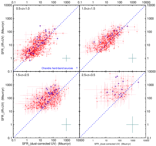
Figure 1.— Comparison between SFR_IR+UV and SFR_corrected-UV for galaxies detected in the MIPS 24$\mu$m image for each redshift bin. Squares represent X-ray sources detected in the Chandra hard-band image. Typical errors of the SFR_IR+UV and SFR_corrected-UV are shown at the bottom right corner of each panel.

4.1. SFR based on MIPS 24$\mu$m flux

Public MIPS 24$\mu$m data for the GOODS-North (DR1+, M. Dickinson et al., in preparation) was used for the MIR photometry. Since this image is very deep and its PSF size is relatively large (FWHM $\sim$ 5.4 arcsec), the source confusion occurs for many objects. Following Le Floc’h et al. (2005), we use the IRAF/DAOPHOT package (Stetson, 1987) in order to deal with these blended sources properly. The DAOPHOT software is based on the PSF fitting technique and allows us to fit blended sources in a crowded region simultaneously and then derive the flux of each object from the scaled fitted PSF. An empirical PSF was constructed from bright isolated point sources. We used the positions of the sample galaxies on the high-resolution MOIRCS $K_{s}$-band image as a prior for the centers of the fitted PSFs in the photometry. The background noise was estimated by measuring sky fluxes at random positions on the image. For sources whose residual of the PSF fitting was significantly larger than the background noise, we added the fitting residual to the photometric error. We set a detection threshold of 5$\sigma$, which corresponds to $\sim 20\mu$Jy in most cases where the residual of the fitting is negligible.

In order to convert the MIPS 24$\mu$m flux to the total IR luminosity (8-1000 $\mu$m), we used SED templates of star-forming galaxies provided by Dale & Helou (2002). The model templates cover a wide range of SED shapes, allowing for different heating levels of the interstellar dust by the radiation field. Following Wuyts et al. (2008) and Damen et al. (2009a), we calculated the total IR luminosity for each object using the all templates with the range from $\alpha=1$ to $\alpha=2.5$. $\alpha$ is defined by $dM(U)\sim U^{-\alpha}dU$, where $M(U)$ represents the dust mass headed by an intensity U of the radiation field (Dale & Helou, 2002). Then we averaged the calculated values for the different $\alpha$ in a logarithmic scale and adopted as a best estimate for the IR luminosity. The variation from the value for $\alpha=1$ to that for $\alpha=2.5$ was taken into account in the computation of the error of the total IR luminosity. For objects without spectroscopic redshift, we also estimated the effect of the uncertainty of the photometric redshift by calculating the IR luminosity over the possible ranges of redshift, and added it to the error.

We converted the derived total IR luminosity to a SFR_IR using the Kennicutt (1998)’s relation

$$SFR_{\rm IR}\ (M_{\odot}\ yr^{-1})=4.5\times 10^{-44}\ L_{\rm IR}(erg\ s^{-1}).$$ (1)

Salpeter IMF with lower and upper mass limits of 0.1 and 100 M_⊙ is assumed. The limiting flux of $\sim 20\mu$Jy mentioned above corresponds to $\sim 7$ M_⊙/yr at $z=1$, $\sim 40$ M_⊙/yr at $z=2$, and $\sim 300$ M_⊙/yr at $z=3$. The number of objects detected in the MIPS 24 $\mu$m image in each redshift bin is 626 at $0.5<z<1.0$, 408 at $1.0<z<1.5$, 417 at $1.5<z<2.5$, and 84 at $2.5<z<3.5$, respectively.

4.2. SFR based on rest-frame 2800 Å  luminosity

The rest-frame 2800 Å luminosity for each object was calculated from the same best-fit SED template as used in the estimate of the photometric redshift and stellar mass. Since our multi-band photometric data cover completely the rest-frame 2800 Å for $0.5<z<3.5$, the estimated rest-frame 2800 Å luminosity is a robust quantity, especially in the case where a galaxy is detected in both bands which straddle the rest-frame 2800 Å. We calculated the confidence interval for it in the SED fitting procedure. In order to derive the dust-corrected UV luminosity, we also used E(B-V) of the same best-fit SED template. Since E(B-V) is often degenerated with other parameters of stellar population such as age and metallicity in the SED fitting, the dust-corrected UV luminosity tends to have larger errors than the dust-uncorrected one. Note that our lower limit of the model age of 50 Myr in the SED fitting affects the estimated E(B-V), thus the dust-corrected UV luminosity and SFR. We will discuss the effect of the age limit on SFR in Section 5.1.

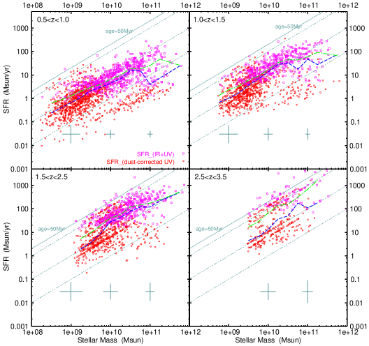
Figure 2.— SFR vs. M_star for our stellar mass limited sample for each redshift bin. Squares show galaxies with SFR_IR+UV derived from the 24 $\mu$m fluxes, while circles represent objects undetected in the MIPS 24 $\mu$m image, with SFR_corrected-UV derived from the dust-corrected rest-frame UV luminosity. Median errors of the SFR and stellar mass at each mass are shown as the crosses at the bottom of each panel. Dotted lines represent SFR/M${}_{\rm star}=$ 1/50 Myr^-1 (see text for details). Double-dotted dashed lines show SFR/M${}_{\rm star}=$ 0.1, 1, 10 Gyr^-1. Blue dashed lines show the median SFR at each stellar mass. Green dotted-dashed lines represent the results of the linear fitting for star-forming galaxies. In the panel of the $2.5<z<3.5$ bin, the lower line shows the result for galaxies with $\log$(SFR/M_star) $>$ -0.5, and upper one shows that for galaxies with $\log$(SFR/M_star) $>$ 0.25.

We converted the dust-uncorrected and dust-corrected rest-frame 2800 Å luminosities into SFRs using the calibration by Kennicutt (1998)

$$SFR_{\rm UV}\ (M_{\odot}\ yr^{-1})=1.4\times 10^{-28}\ L_{\nu}(erg\ s^{-1}\ Hz^{-1}).$$ (2)

The SFR estimated from the dust-uncorrected UV luminosity accounts for the unobscured light from young stars and is added to the SFR_IR estimated from the 24$\mu$m flux for objects detected in the MIPS 24$\mu$m image. We refer to the combined value as SFR_IR+UV in the following. The SFR estimated from the dust-corrected UV luminosity (hereafter SFR_corrected-UV) can be calculated for all the sample.

4.3. Comparison between SFR_IR+UV and SFR_corrected-UV

Figure 1 shows a comparison between SFR_IR+UV and SFR_corrected-UV for galaxies detected in the MIPS 24$\mu$m image. Given the uncertainty, these two estimates agree well with each other especially in low-redshift bins. At low SFR, however, SFR_IR+UV tends to be higher than SFR_corrected-UV, and the systematic offset seems to become larger with redshift. The mean and standard deviation of $\log(SFR_{\rm IR+UV}/SFR_{\rm corrected-UV})$ for all objects with the MIPS 24$\mu$m detection are $0.19\pm 0.39$ at $0.5<z<1.0$, $0.25\pm 0.37$ at $1.0<z<1.5$, $0.37\pm 0.49$ at $1.5<z<2.5$, and $0.63\pm 0.64$ at $2.5<z<3.5$. Franx et al. (2008) reported a similar trend in the comparison between the SFRs derived from the MIPS 24$\mu$m flux and the SED fitting.

In the conversion from the 24$\mu$m flux into the total IR luminosity, we don’t take into account the luminosity-dependent shapes of the IR SED found in local galaxies (e.g., Chary & Elbaz, 2001), following Wuyts et al. (2008) and Damen et al. (2009a). Therefore SFR_IR+UV could be overestimated for galaxies with low IR luminosity (SFR) and underestimated for those with high IR luminosity, if the luminosity-dust temperature (IR color) relation for nearby galaxies holds for galaxies at higher redshift. On the other hand, there are several studies that suggest that high-z active star-forming galaxies do not form such a relation and galaxies with L${}_{\rm IR}>10^{12}$L_⊙ (ULIRGs) at high redshift have cooler average dust temperatures than those in the local universe (e.g., Symeonidis et al., 2009; Muzzin et al., 2010). Furthermore, it is reported that bright 24 $\mu$m sources at $z\sim 2$ have higher polycyclic aromatic hydrocarbon (PAH) luminosity relative to the total IR luminosity than the local ULIRGs with similar IR luminosity (Huang et al., 2009; Murphy et al., 2009). Since the MIPS 24 $\mu$m band samples the PAH emissions in 6-9 $\mu$m region at $z\gtrsim 1.5$, higher L_PAH/L_IR ratios than those for the local ULIRGs could lead to a overestimation of SFR for these high-z galaxies if one converts 24 $\mu$m fluxes into the SFRs using the local luminosity-dust temperature relation.

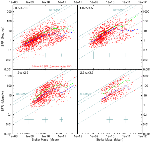
Figure 3.— The same as Figure 2 except that SFR_corrected-UV is used for all the sample.

It should be noted that the MIR flux may also be powered partly by AGN (e.g., Nardini et al., 2008). We showed objects detected in the Chandra hard-band image of the CDF-North (Alexander et al., 2003) as squares in Figure 1. Those objects detected in the hard-band of Chandra have slightly higher SFR_IR+UV/SFR_corrected-UV ratios; the mean and standard deviation of $\log(SFR_{\rm IR+UV}/SFR_{\rm corrected-UV})$ for those objects are $0.31\pm 0.38$ at $0.5<z<1.0$, $0.37\pm 0.35$ at $1.0<z<1.5$, $0.54\pm 0.32$ at $1.5<z<2.5$, and $0.80\pm 0.66$ at $2.5<z<3.5$. SFR_IR+UV for those sources could be overestimated due to the AGN contribution, although SFR_IR+UV tends to be higher than SFR_corrected-UV especially at high redshift even if we exclude the Chandra hard-band sources.

On the other hand, the dust-corrected UV luminosity might be underestimated for heavily obscured galaxies such as ULIRGs at low and high redshifts (e.g., Goldader et al., 2002; Papovich et al., 2006; Reddy et al., 2010). If a galaxy has star-forming regions from which one can detect no UV light at all due to the heavy dust obscuration, only UV light from relatively less-obscured regions contributes the observed SED, which could result in the underestimate of the dust extinction.

Since the calibration by Kennicutt (1998) we used for the conversion from the rest-frame 2800 Å luminosity into SFR is derived assuming that SFR has remained constant over a timescale of $\sim 100$ Myr and that the luminosity is dominated by young O and B stars, SFR could be overestimated for relatively quiescent galaxies. For such galaxies, older stellar population than O and B stars could contribute significantly to the rest-frame 2800 Å luminosity (e.g., Dahlen et al., 2007). Therefore SFR_corrected-UV could be systematically overestimated for galaxies with low SFRs relative to their stellar mass.

Keeping in mind the possible systematic errors, we show both results with SFR_IR+UV for objects detected in the MIPS 24$\mu$m image and SFR_corrected-UV for those without the MIPS detection, and with SFR_corrected-UV for all the sample in the following section.

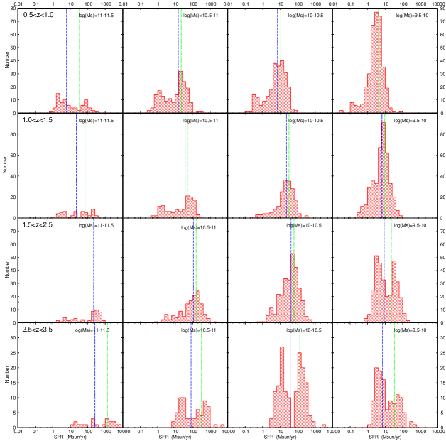
Figure 4.— SFR distribution for galaxies in each stellar mass and redshift bin. SFR_IR+UV is used if a galaxy is detected in the MIPS 24$\mu$m image and SFR_corrected-UV is used for objects without the 24$\mu$m detection. Dashed and dotted-dashed lines show the median and average SFRs for each mass and redshift bin.

5. Results

5.1. SFR as a function of Stellar Mass at $0.5<z<3.5$

Figure 2 and 3 show the SFR as a function of M_star for the stellar mass selected sample in the four redshift bins. Figure 2 represents the case where SFR_IR+UV is used if a galaxy is detected in the MIPS 24$\mu$m image and SFR_corrected-UV is used for those without the 24$\mu$m detection, and Figure 3 represents the case where SFR_corrected-UV is used for all the sample. A dotted line in each redshift panel represents SFR/M${}_{\rm star}=$ 1/50 Myr^-1. In the calculation of the SFR_corrected-UV, both the rest-frame 2800 Å luminosity and the E(B-V) were estimated from the SED fitting. The stellar mass is also based on the same best-fit SED model. Since SFR/M_star of the model SED cannot exceed the inverse of the age for the monotonically decaying SFR models (SFR/M_star roughly equals the inverse of the age for the constant SFR models if one ignores the stellar mass loss due to the super nova or stellar wind), the lower limit of the model age leads to the upper limit for the SFR/M_star. Therefore, the lower limit of age $>$ 50 Myr in the SED fitting mentioned above causes the upper limit of SFR_corrected-UV/M${}_{\rm star}<$ 1/50 Myr^-1 ($=$ 20 Gyr^-1). On the other hand, the SFR_IR+UV is not affected by this limit, because the SFR based on the 24 $\mu$m flux are independent of the result of the SED fitting for the stellar emission. Since there are only a few objects whose SFR_IR+UV significantly exceeds this limit in high-redshift bins in Figure 2, we believe that the lower limit of the model age does not significantly bias the distribution of the SFR_corrected-UV as a function of M_star.

In Figure 2 and 3, we plot the median and average of SFR at each mass as a dashed and dotted-dashed lines, respectively, to examine in detail the stellar mass dependence of the SFR. At M${}_{\rm star}\lesssim 10^{10.5}$ M_⊙, more massive galaxies tend to have higher SFRs in all redshift bins, although there is a substantial scatter at each mass. The median and average SFRs of these galaxies increase with M_star. On the other hand, the trend becomes less clear at M${}_{\rm star}\gtrsim 10^{10.5}$ M_⊙;the median SFR does not significantly increase with M_star, especially in the case with SFR_corrected-UV for all the sample (Figure 3). There are massive galaxies with relatively low SFRs similar with low-mass galaxies, while galaxies with higher SFRs which follow the trend at lower M_star also exist.

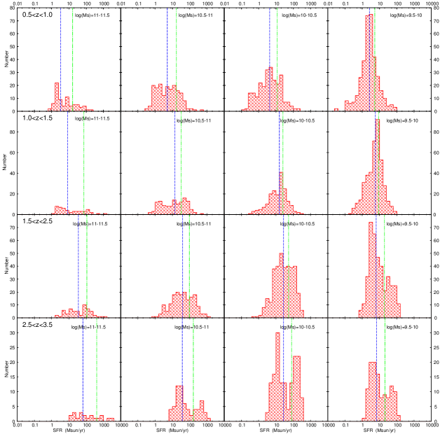
Figure 5.— The same as Figure 4 except that SFR_corrected-UV is used for all the sample.

We note that the SFR distribution at a fixed M_star shifts to higher values with increasing redshift at least at $z<2.5$ in Figure 2 and 3. Figure 4 and 5 show the SFR distribution for each stellar mass and redshift bin. At $z<2.5$, the shift of the SFR distribution with redshift is seen in all mass bins in the both figures, although there are galaxies with relatively wide range of SFR in each mass and redshift bin. Furthermore, it is seen that more massive galaxies show stronger evolution of the SFR in the both cases with different SFR indicators.

At $2.5<z<3.5$, galaxies with $M_{\rm star}=$ 10^9.5–10¹¹ M_⊙ show a bimodality in the SFR, and the SFR distribution does not concentrate around the median or average value (Figure 4 and 5). The SFRs of the both high-SFR and low-SFR groups of the bimodality seem to increase with M_star. Since the bimodality is also seen in the case where the SFR_corrected-UV is used for all the sample, it is not due to the effect of the detection limit of the MIPS 24 $\mu$m data. While the median SFRs of galaxies at $2.5<z<3.5$ are similar with those at $1.5<z<2.5$ in all stellar mass bins, the average SFRs of these galaxies tend to be higher than those at $1.5<z<2.5$ due to galaxies with very high SFRs, especially at high mass.

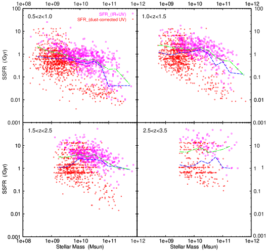
Figure 6.— Specific star formation rate (SFR/M_star) vs M_star for our stellar mass limited sample for each redshift bin. SFR_IR+UV is used if a galaxy is detected in the MIPS 24$\mu$m image and SFR_corrected-UV is used for objects without the 24$\mu$m detection. Symbols are the same as Figure 2.

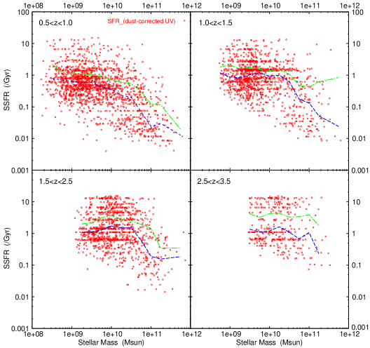
Figure 7.— The same as Figure 6 except that SFR_corrected-UV is used for all the sample.

5.2. SSFR vs M_star

In Figure 6 and 7, we show SSFR vs M_star for our sample in the both cases with the different SFR indicators. At M${}_{\rm star}\lesssim 10^{10.5}$ M_⊙, the median and average of the SSFR are nearly independent of M_star at least at $z>1$, although the median and average values slightly decrease with M_star in the lowest redshift bin. This indicates that the relation between SFR and M_star for galaxies with M${}_{\rm star}\lesssim 10^{10.5}$ M_⊙ has a logarithmic slope of $\sim$ 1 (slightly less than 1 for the lowest redshift bin). On the other hand, the median and average SSFRs decrease with M_star at M${}_{\rm star}\gtrsim 10^{10.5}$ M_⊙, except for the average SSFR in the $2.5<z<3.5$ bin.

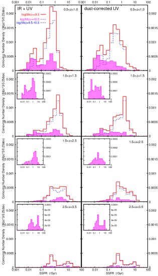
Figure 8.— Distribution of the specific star formation rate (SFR/M_star) for galaxies with M${}_{\rm star}>10^{9.5}$ M_⊙ in each redshift bin. Left panels show the case where SFR_IR+UV is used for galaxies detected at 24 $\mu$m and SFR_corrected-UV for the other objects, while right panels show the case where SFR_corrected-UV is used for all the sample. Long dashed line (Magenta) represents galaxies with M${}_{\rm star}>10^{10.5}$ M_⊙, and short dashed line (blue) shows those with M${}_{\rm star}=10^{9.5-10.5}$ M_⊙. The insets represent the zoom-up of the plots for galaxies with M${}_{\rm star}>10^{10.5}$ M_⊙.

In order to investigate the evolution of the SSFR, we show a distribution of SSFR for the cases with the different SFR indicators in Figure 8. We use the V_max method to calculate the comoving number density. K09 calculated the V_max for the $K$-band magnitude limit ($K=23$ for the wide field or $K=24$ for the deep field) by using the best-fit model template for each object (see Section 3.3 in K09 for details). In the figure, we use only galaxies with M${}_{\rm star}>10^{9.5}$ M_⊙ for a fair comparison among the different redshift bins. We also show galaxies with M${}_{\rm star}=$ 10^9.5-10.5 M_⊙ and with M${}_{\rm star}>10^{10.5}$ M_⊙ separately. It is seen that the distribution of the SSFR shifts to higher values with redshift, while the comoving number density of galaxies decreases.

At $2.5<z<3.5$, the bimodality in the SFR mentioned above is also seen in the SSFR distribution, as a more simple form. There are a group of galaxies with high SSFRs of SFR/M${}_{\rm star}\sim$ 10 Gyr^-1 and that of galaxies with relatively low SSFRs of SFR/M${}_{\rm star}\sim$ 0.6 Gyr^-1. Thus, a constant SSFR of SFR/M${}_{\rm star}\sim$ 2 Gyr^-1 can divide between the two populations independent of M_star in the both cases with the different SFR indicators.

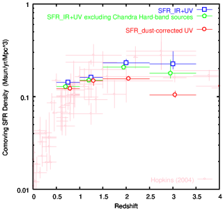
Figure 9.— Evolution of the total cosmic SFR density for our stellar mass limited sample for the cases with the different SFR indicators. The case with SFR_IR+UV where the Chandra hard-band sources are excluded is also shown (the result with SFR_corrected-UV does not change significantly if we exclude the Chandra hard-band sources). Small open circles show the compilation from Hopkins (2004).

5.3. Contribution to the Cosmic SFR Density

Here we examine the contribution to the cosmic SFR density (hereafter, SFRD) of galaxies with different stellar masses. We use the same V_max as used in Section 5.2 to estimate the SFRD. At first, we show the integrated SFRD for our sample and compare it with a compilation by Hopkins (2004) in Figure 9. The integrated SFRD was calculated from the sample limited by the stellar mass which depends on redshift (Section 3) and was not extrapolated down to lower mass. Therefore the SFRD at higher redshift in the figure was integrated only down to the higher stellar mass limit. Since the contribution of galaxies with $M_{\rm star}<10^{10}$ M_⊙ seems to be negligible even at high redshift as we show below, however, the effect of the systematically higher mass limit at high redshift is expected to be small.

In Figure 9, we plot the both results with the different SFR indicators and also show the case with SFR_IR+UV where Chandra hard-band sources are excluded. The integrated SFRDs for our sample increase with redshift up to $z\sim 2$ and are constant or slightly decrease between $z\sim 2$ and $z\sim 3$. They range within the compilation by Hopkins (2004) over $0.5<z<3.5$, except for a lower SFRD at $z>1.5$ in the case with SFR_corrected-UV for all the sample. $SFR_{\rm corrected-UV}$ for galaxies at high redshift might be underestimated due to the heavy obscuration (Section 4.3).

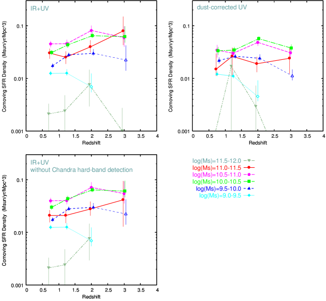
Figure 10.— Contributions of galaxies in different stellar mass ranges to the cosmic SFR density as a function of redshift. Upper left and right panels show the cases with the different SFR indicators. Bottom left panel represents the case with SFR_IR+UV where the Chandra hard-band sources are excluded. Open symbols mean that the incompleteness due to the stellar mass limit could be significant for the redshift bin.

Figure 10 shows the contribution to the cosmic SFRD of galaxies in the different ranges of stellar mass. In the all redshift range, galaxies with M${}_{\rm star}=10^{10-11}$ M_⊙ dominate the cosmic SFRD; their contribution is about 1/2 – 2/3 of the total SFRD. The increase of the cosmic SFRD with redshift up to $z\sim 2$ seems to reflect mainly the evolution of the contribution of galaxies in this mass range.

In the case with SFR_IR+UV, the contribution of massive galaxies with M${}_{\rm star}=10^{11-11.5}$ M_⊙ shows stronger evolution at $z\gtrsim 1.5$ than that of galaxies with M${}_{\rm star}=10^{10-11}$ M_⊙ and continues to increase up to $z\sim 3$. These massive galaxies significantly contribute the cosmic SFRD at $2.5<z<3.5$, while the contribution of these galaxies is relatively small at $z\lesssim 2$. In the case where the Chandra hard-band sources are excluded, the contribution of these massive galaxies is slightly lower and its evolution is milder, although the contribution becomes significant at $z\sim 3$ even in this case. This is because the X-ray AGN is preferentially associated with massive galaxies (e.g., Best et al., 2005) and because the fraction of objects detected at hard X-ray in massive galaxies becomes very high at $z\gtrsim 2$ (Yamada et al., 2009; Brusa et al., 2009). While the SFR_IR+UV of the Chandra hard-band sources could be overestimated due to the contribution of AGN, the exclusion of these galaxies might cause the underestimate of the contribution of massive galaxies to the SFRD if a significant fraction of the IR luminosity of these galaxies arises from star formation activities. In the case where SFR_corrected-UV is used for all the sample, the contribution of these galaxies with M${}_{\rm star}=10^{11-11.5}$ M_⊙ has a large uncertainty even at low redshift and its evolution is less clear. This is partly because the large error of the SFR for heavily obscured galaxies with high SFR. In particular, the contribution at $1.0<z<1.5$ is strongly affected one such object with SFR${}_{\rm corrected-UV}>$ 1000 M_⊙/yr (Figure 3).

The contribution of galaxies with M${}_{\rm star}<10^{10}$ M_⊙ seems to be small at any redshift, although the completeness limit for our sample becomes $\sim 10^{9.5-10}$ M_⊙ at $z\sim 3$. The contribution of galaxies with M${}_{\rm star}=10^{9.5-10}$ M_⊙ is $\sim$ 15% of the total SFRD at $0.5<z<3.5$ and evolves similarly with that for galaxies with M${}_{\rm star}=10^{10-11}$ M_⊙. Galaxies with M${}_{\rm star}>10^{11.5}$ M_⊙ have a negligible contribution, although there are only a few such very massive galaxies in each redshift bin and the uncertainty of the contribution is very large.

6. Discussion

6.1. Comparison with Other Studies at $z<2.5$

We have investigated the distribution of SFR as a function of stellar mass for galaxies at $0.5<z<3.5$, using the stellar mass limited sample based on the very deep NIR imaging data of the MODS. We here compare our results in the MODS field with previous studies mainly at $z<2.5$.

Several studies examined the relation between SFR and stellar mass of star-forming galaxies, and found that more massive galaxies tend to have higher SFRs at $z\sim 1$ (Noeske et al., 2007; Elbaz et al., 2007) and at $z\sim 2$ (Santini et al., 2009; Daddi et al., 2007; Pannella et al., 2009; Dunne et al., 2009). At M${}_{\rm star}\lesssim 10^{10.5}$ M_⊙, we found a similar trend in our sample at $0.5<z<2.5$, and confirmed the same trend at $2.5<z<3.5$ although the SFR distribution shows the bimodality and does not concentrate around the average value. At M${}_{\rm star}\gtrsim 10^{10.5}$ M_⊙, there are massive galaxies with similar SFRs with lower-mass galaxies in our stellar mass-selected sample, while galaxies with higher SFRs which follow the trend at lower M_star also exist. If we excluded galaxies with relatively low SFRs as a quiescent population, we could consider the relation between SFR and stellar mass continues to high mass for star-forming galaxies, which has been reported in other studies.

Our result that the SFR (SSFR) distribution at a fixed M_star shifts to higher values with increasing redshift is also consistent with these previous studies. For example, Pannella et al. (2009) estimated an average SFR as a function of M_star for star-forming BzK galaxies with $K\lesssim$ 21.2 at $z\sim 2$ in the COSMOS field by performing a stacking analysis of 1.4 GHz radio continuum. They pointed out that the SSFR of these star-forming galaxies show a evolution of a factor of $\sim$ 4 between $z=1.4$ and $z=2.3$. Using the stellar mass-selected sample whose limiting mass reaches $\sim$ 10^9.5–10¹⁰ M_⊙ even at $z\sim 3$, we found that more massive galaxies show stronger evolution of the SFR at $z\gtrsim 1$.

We found the median and average SSFRs of galaxies is nearly independent of M_star at M${}_{\rm star}\lesssim 10^{10.5}$ M_⊙ at $z>1$, while they slightly decrease with M_star at $0.5<z<1.0$. This indicates that the logarithmic slope of the relation between SFR and M_star is $n\sim 1$ ($n\lesssim 1$ for $0.5<z<1.0$). Other studies reported the similar slope of the SFR-M_star relation, although there is some variance among the studies in the observed slope and scatter of the relation (Daddi et al., 2007; Santini et al., 2009; Pannella et al., 2009; Elbaz et al., 2007; Noeske et al., 2007). The variance might be explained by differences in the sample selection or the SFR indicators among the studies.

The SSFR independent of M_star at M${}_{\rm star}<10^{10.5}$ M_⊙ means that the stellar mass growth by star formation activities in each galaxy is similar among galaxies with different masses. Using the same sample as this study, K09 investigated the evolution of the galaxy stellar mass function (SMF), and found that the low-mass slope of the SMF becomes steeper with redshift at $1\lesssim z\lesssim 3$. The nearly constant mass growth rate by star formation expected from the slope of n $\sim$ 1 implies that star formation in each galaxy does not significantly change the low-mass slope with time. If such mass-independent SSFR continues down to lower mass than the stellar mass limit of our sample in the high redshift bins, additional mechanisms such as the hierarchical merging, which destroys small galaxies and builds more massive ones, might be needed in order to reproduce the evolution of the low-mass slope (K09).

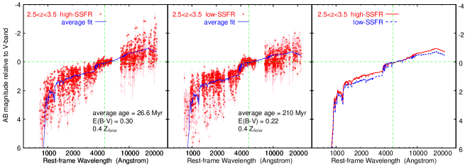
Figure 11.— Rest-frame broad-band SEDs of star-forming galaxies at $2.5<z<3.5$. Left and middle panels show those with $\log$(SFR_IR+UV/M_star) $>$ 0.25 (the high-SSFR population) and those with $\log$(SFR_IR+UV/M_star) $=$ -0.5 – 0.25 (the low-SSFR population). Errorbars represent the 1$\sigma$ photometric uncertainties and arrows indicate the 2$\sigma$ upper limits. Solid line in each panel shows the best-fit SED model for all the data points. Average stellar age, color excess, and metallicity of the best-fit model are also shown in the panels. Right panel shows a comparison between these average SEDs for the high- and low-SSFR populations. If we use the SFR_corrected-UV for all the sample, the best-fit SEDs for the high- and low-SSFR populations are almost the same as seen in this figure.

6.2. Bimodality in SSFR of star-forming galaxies at $2.5<z<3.5$

We found the bimodality in the SSFR distribution of galaxies at $2.5<z<3.5$, which can be divided into two populations by a constant SSFR of $\sim$ 2 Gyr^-1. One population consists of galaxies with SFR/M${}_{\rm star}\sim$ 0.5–1 Gyr^-1, and those with SFR/M${}_{\rm star}\sim$ 10 Gyr^-1 belong to the other population. For the SSFR of galaxies at $z>2.5$, the SFR and M_star of Lyman Break Galaxies (LBGs) have been investigated by several studies. Magdis et al. (2010) reported that LBGs detected in the IRAC 3.6 $\mu$m and 4.5 $\mu$m bands at $z\sim 3$ show the SFR-M_star relation with a slope of n $\sim$ 0.9 and a considerable scatter, and that their median SSFR of $\sim$ 4.5 Gyr^-1 is higher than those at lower redshifts, while several observational studies suggest that the SFR-M_star relation for Lyman Break Galaxies at $4\lesssim z\lesssim 7$ is similar with that at $z\sim 2$ (Daddi et al., 2009; Stark et al., 2009; González et al., 2010). The range of the SSFR of LBGs in Magdis et al. (2010) is similar with galaxies at $2.5<z<3.5$ in our sample, although most of LBGs in their sample have M${}_{\rm star}\gtrsim 10^{10.5}$ M_⊙ probably due to the IRAC selection and the number of galaxies with low SSFR is relatively small.

Dutton et al. (2010) constructed a semi-analytic model for disk galaxies and suggested that the evolution of the normalization of the SFR-M_star relation for these disk galaxies at $z\lesssim 2$ closely follows the evolution in the gas (and dark matter) accretion rate. They predicted that the normalization continues to increase with redshift up to $z>2$, if the SFR follows the gas accretion rate at such high redshift. The SFR of the high-SSFR population at $2.5<z<3.5$ may be related with the evolution of the gas accretion rate at such high redshift, although the SSFR of $\sim$ 10 Gyr^-1 at $z\sim 3$ is higher than the model prediction by Dutton et al. (2010).

Recently, Daddi et al. (2010) reported a bimodality in the SFR relative to the gas mass for star-forming galaxies at low and high redshifts and proposed that the star formation efficiency would be different between disk and starburst galaxies because different modes of star formation work in the two populations. The high-SSFR population at $2.5<z<3.5$ in our sample might correspond to such starburst galaxies. For example, the starburst sequence consists of sub-millimeter galaxies (SMGs) at high redshift as well as local ULIRGs in Daddi et al. (2010) and several studies suggest that high-z SMGs tend to show relatively high SSFRs (e.g., Takagi et al., 2008; Daddi et al., 2009). There are 23 SCUBA sources in the MODS field (Pope et al., 2006), and all but one (GN10, Wang et al., 2007; Wang et al., 2009) have counterparts in the $K$-selected catalog of the MODS. Of 22 sources detected in the $K$-band image, 6 SCUBA sources lie at $2.5<z<3.5$ (3 with spectroscopic redshift and 3 only with photometric redshift), all but one hard X-ray source (GN22, Laird et al., 2010) belong to the high-SSFR population with SFR/M${}_{\rm star}\sim$ 10 Gyr^-1. Figure 11 shows the rest-frame broad-band SEDs of star-forming galaxies at $2.5<z<3.5$ on the high- and low-SSFR populations. We defined the high-SSFR population as galaxies with $\log$(SFR/M_star[Gyr^-1]) $>$ 0.25 and the low-SSFR population as those with $\log$(SFR/M_star) $=$ -0.5–0.25, respectively. The high-SSFR population shows weaker Balmer break feature and redder color at long wavelength, which indicates that these galaxies are younger and dustier, while the overall slope of SEDs and scatters among the objects are similar between the two populations. Those objects in the high-SSFR population might have higher star formation efficiency than ordinary star-forming (disk) galaxies.

6.3. Evolution of Cosmic SFRD and Stellar Mass Assembly of Galaxies

In Section 5.3, we saw that galaxies with M${}_{\rm star}=10^{10-11}$ M_⊙ dominate the cosmic SFRD at $0.5<z<3.5$, and the contribution of galaxies with M${}_{\rm star}=10^{11-11.5}$ M_⊙ increases with redshift even at $z\gtrsim 2$ and becomes significant at $z\sim 3$. On the other hand, K09 investigated the contribution of galaxies in different mass ranges to the cosmic stellar mass density, and found that galaxies with M${}_{\rm star}\sim 10^{10.5-11.5}$ M_⊙ ($10^{10-11.5}$ M_⊙ at $z\sim 3$) dominate the cosmic stellar mass density (Figure 17 in K09). Considering the nearly constant SSFR among (star-forming) galaxies with different stellar masses discussed in Section 6.1, the result that galaxies with $10^{10-11.5}$ M_⊙ dominate the cosmic SFRD is qualitatively consistent with the dominant contribution of these galaxies in the stellar mass density. Major star formation in the universe at $1\lesssim z\lesssim 3$ seems to occur in galaxies with stellar mass which dominates the cosmic stellar mass density or those with slightly lower stellar mass.

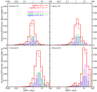
Figure 12.— Contributions of galaxies in different SSFR ranges to the cosmic SFR density in each redshift bin for the case where SFR_IR+UV is used for galaxies detected at 24 $\mu$m and SFR_corrected-UV for the other objects. Only galaxies with M${}_{\rm star}>10^{9.5}$ M_⊙ are used for all the redshift bins. Thick solid line shows galaxies with M${}_{\rm star}>10^{9.5}$ M_⊙ and thin solid line represents galaxies with M${}_{\rm star}=10^{10-11.5}$ M_⊙. Dotted (magenta), long dashed (green), and short dashed (blue) lines represent galaxies with M${}_{\rm star}=10^{11-11.5}$, $10^{10.5-11}$, and $10^{10-10.5}$ M_⊙, respectively.

The cosmic SFRD increases with redshift from $z\sim 0$ up to $z\sim 2$ and is roughly constant or slightly decreases between $z\sim 2$ and $z\sim 3$ (e.g., Hopkins & Beacom, 2006). The evolution of the cosmic SFRD roughly follows that of galaxies with M${}_{\rm star}=10^{10-11}$ M_⊙, which dominate the SFRD (Figure 9 and 10). In Figure 4 and 5, the average SFR per galaxy for those with M${}_{\rm star}=10^{10-11}$ M_⊙ increases with redshift up to $z\sim 3$, but the evolution between $z\sim 2$ and $z\sim 3$ seems to be weaker than that at lower redshift. On the other hand, K09 investigated the evolution of the number density of galaxies in different mass ranges, and showed that the number density of these galaxies decreases gradually with redshift (Figure 16 in K09). At $z\lesssim 2$, the increase in the average SFR per galaxy with redshift overwhelms the decrease in the number density, and therefore the contribution of these galaxies to the total SFRD increases with redshift. At $2\lesssim z\lesssim 3$, the evolution of the SFR per galaxy becomes weaker, while the number density continues to decrease even at such high redshift. Then these two roughly balances, and the SFRD is nearly constant or slightly decreases with redshift. For galaxies with M${}_{\rm star}=10^{11-11.5}$ M_⊙, the average SFR evolves more strongly between $z\sim 2$ and $z\sim 3$ especially in the case with SFR_IR+UV. The strong evolution of the SFR per galaxy for these massive galaxies continues to overwhelm the decrease in the number density up to $z\sim 3$, although the number density of these galaxies also continues to decrease to $z\sim 3$. As a result, the contribution of these galaxies with M${}_{\rm star}=10^{11-11.5}$ M_⊙ to the SFRD increases with redshift even at $z\gtrsim 2$.

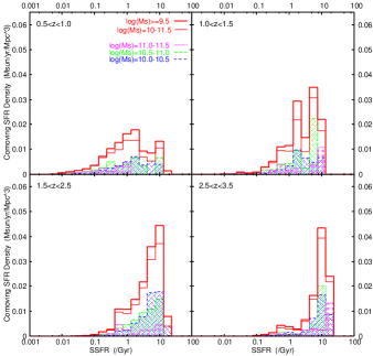
Figure 13.— The same as Figure 12 but for the case where SFR_corrected-UV is used for all the sample.

In other words, the number density of galaxies is relatively small, but the average SFR per galaxy is high at $z\sim 3$. As time goes on, the SFR in each galaxy decreases, while the number density of galaxies at a fixed M_star increases due to the stellar mass growth in galaxies with a wide range of masses. In particular, the SFR in massive galaxies with M${}_{\rm star}=10^{11-11.5}$ M_⊙ decreases rapidly, and a fraction of these galaxies enters into a quiescent phase (massive galaxies with low SSFR in Figure 6 and 7). As a result, the contribution of these galaxies to the SFRD becomes relatively small by $z\sim 2$. At $z\lesssim 2$, the decrease of the SFR in each galaxy with M${}_{\rm star}=10^{10-11}$ M_⊙ overwhelms the increase in the number density, which drives the overall decrease of the cosmic SFRD with time.

In Figure 12 and 13, we show the contribution of galaxies with different SSFRs to the cosmic SFRD in the cases with SFR_IR+UV and SFR_corrected-UV, respectively. It is seen that in galaxies with M${}_{\rm star}=10^{10-11.5}$ M_⊙, those with a relatively narrow range of SSFR ($\lesssim 1$ dex) dominate the cosmic SFRD, especially in the case with SFR_IR+UV. Furthermore, the SSFR of galaxies which dominate the SFRD systematically increases with redshift. In this context, major star formation in the universe at higher redshift seems to be associated with a more rapid growth of stellar mass of galaxies. At $2.5<z<3.5$, in particular, the high-SSFR population with SFR/M${}_{\rm star}\sim$ 10 Gyr^-1, which are relatively small in number (Figure 8), dominate the SFRD. If these objects would be the ’starburst’ galaxies with distinctively higher star formation efficiency than ordinary disk galaxies as discussed in the previous section, these galaxies are expected to grow their stellar mass rapidly and could cause the increase of the number density of massive galaxies at $1\lesssim z\lesssim 3$. There might be a transition in the dominant component of the star formation in the universe between $z\sim 3$ and $z\sim 1$; from starburst in relatively small number of galaxies at $z\sim 3$, which drives a rapid growth of stellar mass, to star formation in many disk galaxies at $z\sim 1$, which leads to a more gradual growth of stellar mass.

7. Summary

We studied SFR as a function of M_star for galaxies at $0.5<z<3.5$ in the GOODS-North field, using the $K$-selected sample from the MODS. The very deep NIR data of the MODS allow us to construct the stellar mass limited sample down to 10^9.5-10 M_⊙ even at $z\sim 3$. The rest-frame 2800 Å luminosity and the MIPS 24 $\mu$m flux were used to estimate the SFRs of the sample galaxies. Using these SFR indicators, we showed the two cases of the results, namely, one case where SFR_IR+UV is used if a galaxy is detected in the MIPS 24$\mu$m image and SFR_corrected-UV is used for those without the 24$\mu$m detection, and the other case where SFR_corrected-UV is used for all the sample.

Main results in this study are as follows.

• More massive galaxies tend to have higher SFRs at M${}_{\rm star}\lesssim 10^{10.5}$ M_⊙ in all redshift ranges. At M${}_{\rm star}\gtrsim 10^{10.5}$ M_⊙, there are galaxies with relatively low SFRs similar with low-mass galaxies, while galaxies with higher SFRs which follow the trend at lower M_star also exist.

• The median and average SSFRs of galaxies is nearly independent of M_star at M${}_{\rm star}\lesssim 10^{10.5}$ M_⊙ at $z>1$, while they slightly decrease with M_star at $0.5<z<1.0$. At M${}_{\rm star}\gtrsim 10^{10.5}$ M_⊙, the median and average SSFRs decrease with M_star.

• The SFR (SSFR) distribution at a fixed M_star shifts to higher values with increasing redshift. More massive galaxies show the stronger evolution of SFR at $z\gtrsim 1$.

• At $2.5<z<3.5$, the bimodality in the SFR and SSFR distributions at each mass is seen. The bimodality is the more simple form in SSFR and can be divided into the two populations by a constant SSFR of $\sim$ 2 Gyr^-1. One population consists of galaxies with SFR/M${}_{\rm star}\sim$ 0.5–1 Gyr^-1, and the other population is the high-SSFR population, to which galaxies with SFR/M${}_{\rm star}\sim$ 10 Gyr^-1 belong. These high- and low-SSFR populations might have different modes of star formation, namely, starburst and more continuous star formation in disks.

• Galaxies with M${}_{\rm star}=10^{10-11}$ M_⊙ dominate the cosmic SFRD at $0.5<z<3.5$. The evolution of these galaxies seems to drive the evolution of the cosmic SFRD, especially at $z\lesssim 2.5$. The contribution of galaxies with M${}_{\rm star}=10^{11-11.5}$ M_⊙ increases strongly with redshift at $z>1.5$ and becomes significant at $z\sim 3$. The contribution of galaxies with M${}_{\rm star}<10^{10}$ M_⊙ is relatively small at any redshift.

• In galaxies with M${}_{\rm star}=10^{10-11.5}$ M_star, those with a relatively narrow range of SSFR ($\lesssim$ 1 dex) dominate the cosmic SFR at $0.5<z<3.5$ especially in the case with SFR_IR+UV. The SSFR of galaxies which dominate the SFRD systematically increases with redshift. At $2.5<z<3.5$, the high-SSFR population dominates the cosmic SFRD. Major star formation in the universe at higher redshift seems to be associated with a more rapid growth of stellar mass of galaxies.

Systematic errors in the SFRs estimated from the 24 $\mu$m flux and the optical-NIR broad-band SED (Section 4.3) could affect some of the above results. More precise measurements of SFR are essential to conclusively confirm the results in this study and to reveal the stellar mass assembly histories of galaxies at $1\lesssim z\lesssim 3$. For example, NIR spectroscopic surveys with sufficiently large sample for the stacking analysis and/or long exposure time enable to estimate directly the dust extinction for the nebular emission lines from the Balmer decrement, and to determine the dust-corrected H$\alpha$ luminosity of star-forming galaxies at that epoch with high accuracy. The forthcoming Herschel and ALMA observations will also provide strong constraints on the shape of the far-IR SED of these galaxies, which allows us to determine the total IR luminosity more precisely.

References

- Alexander et al. (2003) Alexander, D. M., et al. 2003, AJ, 126, 539
- Babbedge et al. (2006) Babbedge, T. S. R., et al. 2006, MNRAS, 370, 1159
- Barger et al. (2008) Barger, A. J., Cowie, L. L., & Wang, W.-H. 2008, ApJ, 689, 687
- Bertin & Arnouts (1996) Bertin E., Arnouts S., 1996, A&AS, 117, 393
- Best et al. (2005) Best, P. N., Kauffmann, G., Heckman, T. M., Brinchmann, J., Charlot, S., Ivezić, Ž., & White, S. D. M. 2005, MNRAS, 362, 25
- Bouché et al. (2010) Bouché, N., et al. 2010, ApJ, 718, 1001
- Bouwens et al. (2007) Bouwens, R. J., Illingworth, G. D., Franx, M., & Ford, H. 2007, ApJ, 670, 928
- Brusa et al. (2009) Brusa, M., et al. 2009, A&A, 507, 1277
- Bruzual & Charlot (2003) Bruzual G., Charlot S., 2003, MNRAS, 344, 1000
- Calzetti et al. (2000) Calzetti, D., Armus, L., Bohlin, R. C., Kinney, A. L., Koornneef, J., & Storchi-Bergmann, T. 2000, ApJ, 533, 682
- Capak et al. (2004) Capak, P., et al. 2004, AJ, 127, 180
- Caputi et al. (2007) Caputi, K. I., et al. 2007, ApJ, 660, 97
- Chabrier (2003) Chabrier, G. 2003, PASP, 115, 763
- Chapman et al. (2005) Chapman, S. C., Blain, A. W., Smail, I., & Ivison, R. J. 2005, ApJ, 622, 772
- Chary & Elbaz (2001) Chary, R., & Elbaz, D. 2001, ApJ, 556, 562
- Cohen (2001) Cohen, J. G. 2001, AJ, 121, 2895
- Cohen et al. (2000) Cohen, J. G., Hogg, D. W., Blandford, R., Cowie, L. L., Hu, E., Songaila, A., Shopbell, P., & Richberg, K. 2000, ApJ, 538, 29
- Connolly et al. (1997) Connolly, A. J., Szalay, A. S., Dickinson, M., Subbarao, M. U., & Brunner, R. J. 1997, ApJ, 486, L11
- Cowie et al. (1999) Cowie, L. L., Songaila, A., & Barger, A. J. 1999, AJ, 118, 603
- Cowie et al. (2004) Cowie, L. L., Barger, A. J., Hu, E. M., Capak, P., & Songaila, A. 2004, AJ, 127, 3137
- Cowie & Barger (2008) Cowie, L. L., & Barger, A. J. 2008, ApJ, 686, 72
- Daddi et al. (2007) Daddi, E., et al. 2007, ApJ, 670, 156
- Daddi et al. (2009) Daddi, E., et al. 2009, ApJ, 694, 1517
- Daddi et al. (2010) Daddi, E., et al. 2010, ApJ, 714, L118
- Dahlen et al. (2007) Dahlen, T., Mobasher, B., Dickinson, M., Ferguson, H. C., Giavalisco, M., Kretchmer, C., & Ravindranath, S. 2007, ApJ, 654, 172
- Dale & Helou (2002) Dale, D. A., & Helou, G. 2002, ApJ, 576, 159
- Dale et al. (2010) Dale, D. A., et al. 2010, ApJ, 712, L189
- Damen et al. (2009a) Damen, M., Labbé, I., Franx, M., van Dokkum, P. G., Taylor, E. N., & Gawiser, E. J. 2009a, ApJ, 690, 937
- Damen et al. (2009b) Damen, M., Förster Schreiber, N. M., Franx, M., Labbé, I., Toft, S., van Dokkum, P. G., & Wuyts, S. 2009b, ApJ, 705, 617
- Dawson et al. (2001) Dawson, S., Stern, D., Bunker, A. J., Spinrad, H., & Dey, A. 2001, AJ, 122, 598
- Dickinson et al. (2003) Dickinson, M., Papovich, C., Ferguson, H. C., & Budavári, T. 2003, ApJ, 587, 25
- Drory & Alvarez (2008) Drory, N., & Alvarez, M. 2008, ApJ, 680, 41
- Dunne et al. (2009) Dunne, L., et al. 2009, MNRAS, 394, 3
- Dutton et al. (2010) Dutton, A. A., van den Bosch, F. C., & Dekel, A. 2010, MNRAS, 405, 1690
- Elbaz et al. (2007) Elbaz, D., et al. 2007, A&A, 468, 33
- Erb et al. (2006) Erb, D. K., Steidel, C. C., Shapley, A. E., Pettini, M., Reddy, N. A., & Adelberger, K. L. 2006, ApJ, 647, 128
- Feulner et al. (2007) Feulner, G., Goranova, Y., Hopp, U., Gabasch, A., Bender, R., Botzler, C. S., & Drory, N. 2007, MNRAS, 378, 429
- Fontana et al. (2006) Fontana, A., et al. 2006, A&A, 459, 745
- Förster Schreiber et al. (2009) Förster Schreiber, N. M., et al. 2009, ApJ, 706, 1364
- Franx et al. (2008) Franx, M., van Dokkum, P. G., Schreiber, N. M. F., Wuyts, S., Labbé, I., & Toft, S. 2008, ApJ, 688, 770
- Geach et al. (2008) Geach, J. E., Smail, I., Best, P. N., Kurk, J., Casali, M., Ivison, R. J., & Coppin, K. 2008, MNRAS, 388, 1473
- Giavalisco et al. (2004) Giavalisco M., et al., 2004, ApJ, 600, L93
- Goldader et al. (2002) Goldader, J. D., Meurer, G., Heckman, T. M., Seibert, M., Sanders, D. B., Calzetti, D., & Steidel, C. C. 2002, ApJ, 568, 651
- González et al. (2010) González, V., Labbé, I., Bouwens, R. J., Illingworth, G., Franx, M., Kriek, M., & Brammer, G. B. 2010, ApJ, 713, 115
- Hopkins (2004) Hopkins, A. M. 2004, ApJ, 615, 209
- Hopkins & Beacom (2006) Hopkins, A. M., & Beacom, J. F. 2006, ApJ, 651, 142
- Huang et al. (2009) Huang, J.-S., et al. 2009, ApJ, 700, 183
- Ichikawa et al. (2007) Ichikawa, T., et al. 2007, PASJ, 59, 1081
- Juneau et al. (2005) Juneau, S., et al. 2005, ApJ, 619, L135
- Kajisawa et al. (2006) Kajisawa, M., et al. 2006, PASJ, 58, 951
- Kajisawa & Yamada (2006) Kajisawa M., Yamada T., 2006, ApJ, 650, 12
- Kajisawa et al. (2009) Kajisawa, M., et al. 2009, ApJ, 702, 1393 (K09)
- Kajisawa et al. (2010) Kajisawa, M., et al. 2010, PASJ, submitted
- Kang et al. (2010) Kang, X., Lin, W. P., Skibba, R., & Chen, D. N. 2010, ApJ, 713, 1301
- Kennicutt (1998) Kennicutt, R. C., Jr. 1998, ARA&A, 36, 189
- Kereš et al. (2005) Kereš, D., Katz, N., Weinberg, D. H., & Davé, R. 2005, MNRAS, 363, 2
- Khochfar & Silk (2009) Khochfar, S., & Silk, J. 2009, ApJ, 700, L21
- Laird et al. (2010) Laird, E. S., Nandra, K., Pope, A., & Scott, D. 2010, MNRAS, 401, 2763
- Le Floc’h et al. (2005) Le Floc’h, E., et al. 2005, ApJ, 632, 169
- Lilly et al. (1996) Lilly, S. J., Le Fevre, O., Hammer, F., & Crampton, D. 1996, ApJ, 460, L1
- Ly et al. (2007) Ly, C., et al. 2007, ApJ, 657, 738
- Madau et al. (1996) Madau, P., Ferguson, H. C., Dickinson, M. E., Giavalisco, M., Steidel, C. C., & Fruchter, A. 1996, MNRAS, 283, 1388
- Madau et al. (1998) Madau, P., Pozzetti, L., & Dickinson, M. 1998, ApJ, 498, 106
- Magdis et al. (2010) Magdis, G. E., Rigopoulou, D., Huang, J.-S., & Fazio, G. G. 2010, MNRAS, 401, 1521
- Magnelli et al. (2009) Magnelli, B., Elbaz, D., Chary, R. R., Dickinson, M., Le Borgne, D., Frayer, D. T., & Willmer, C. N. A. 2009, A&A, 496, 57
- Mannucci et al. (2009) Mannucci, F., et al. 2009, MNRAS, 398, 1915
- Mobasher et al. (2009) Mobasher, B., et al. 2009, ApJ, 690, 1074
- Murphy et al. (2009) Murphy, E. J., Chary, R.-R., Alexander, D. M., Dickinson, M., Magnelli, B., Morrison, G., Pope, A., & Teplitz, H. I. 2009, ApJ, 698, 1380
- Muzzin et al. (2010) Muzzin, A., van Dokkum, P., Kriek, M., Labbe, I., Cury, I., Marchesini, D., & Franx, M. 2010, arXiv:1003.3479
- Nardini et al. (2008) Nardini, E., Risaliti, G., Salvati, M., Sani, E., Imanishi, M., Marconi, A., & Maiolino, R. 2008, MNRAS, 385, L130
- Noeske et al. (2007) Noeske, K. G., et al. 2007, ApJ, 660, L43
- Pannella et al. (2009) Pannella, M., et al. 2009, ApJ, 698, L116
- Papovich et al. (2006) Papovich C., et al., 2006, ApJ, 640, 92
- Pérez-González et al. (2005) Pérez-González, P. G., et al. 2005, ApJ, 630, 82
- Pope et al. (2006) Pope, A., et al. 2006, MNRAS, 370, 1185
- Reddy et al. (2006) Reddy, N. A., Steidel, C. C., Erb, D. K., Shapley, A. E., & Pettini, M. 2006a, ApJ, 653, 1004
- Reddy et al. (2008) Reddy, N. A., Steidel, C. C., Pettini, M., Adelberger, K. L., Shapley, A. E., Erb, D. K., & Dickinson, M. 2008, ApJS, 175, 48
- Reddy et al. (2010) Reddy, N. A., Erb, D. K., Pettini, M., Steidel, C. C., & Shapley, A. E. 2010, ApJ, 712, 1070
- Salpeter (1955) Salpeter, E. E. 1955, ApJ, 121, 161
- Santini et al. (2009) Santini, P., et al. 2009, A&A, 504, 751
- Schiminovich et al. (2005) Schiminovich, D., et al. 2005, ApJ, 619, L47
- Shim et al. (2009) Shim, H., Colbert, J., Teplitz, H., Henry, A., Malkan, M., McCarthy, P., & Yan, L. 2009, ApJ, 696, 785
- Stark et al. (2009) Stark, D. P., Ellis, R. S., Bunker, A., Bundy, K., Targett, T., Benson, A., & Lacy, M. 2009, ApJ, 697, 1493
- Steidel et al. (1999) Steidel, C. C., Adelberger, K. L., Giavalisco, M., Dickinson, M., & Pettini, M. 1999, ApJ, 519, 1
- Stetson (1987) Stetson, P. B. 1987, PASP, 99, 191
- Suzuki et al. (2008) Suzuki, R., et al. 2008, PASJ, 60, 1347
- Symeonidis et al. (2009) Symeonidis, M., Page, M. J., Seymour, N., Dwelly, T., Coppin, K., McHardy, I., Rieke, G. H., & Huynh, M. 2009, MNRAS, 397, 1728
- Takagi et al. (2008) Takagi, T., Ono, Y., Shimasaku, K., & Hanami, H. 2008, MNRAS, 389, 775
- Treu et al. (2005) Treu, T., Ellis, R. S., Liao, T. X., & van Dokkum, P. G. 2005, ApJ, 622, L5
- Wang et al. (2007) Wang, W.-H., Cowie, L. L., van Saders, J., Barger, A. J., & Williams, J. P. 2007, ApJ, 670, L89
- Wang et al. (2009) Wang, W.-H., Barger, A. J., & Cowie, L. L. 2009, ApJ, 690, 319
- Wirth et al. (2004) Wirth, G. D., et al. 2004, AJ, 127, 3121
- Wuyts et al. (2008) Wuyts, S., Labbé, I., Schreiber, N. M. F., Franx, M., Rudnick, G., Brammer, G. B., & van Dokkum, P. G. 2008, ApJ, 682, 985
- Yamada et al. (2009) Yamada, T., et al. 2009, ApJ, 699, 1354
- Yan et al. (1999) Yan, L., McCarthy, P. J., Freudling, W., Teplitz, H. I., Malumuth, E. M., Weymann, R. J., & Malkan, M. A. 1999, ApJ, 519, L47
- Yoshikawa et al. (2010) Yoshikawa, T., et al. 2010, ApJ, 718, 112
- Zheng et al. (2007) Zheng, X. Z., Bell, E. F., Papovich, C., Wolf, C., Meisenheimer, K., Rix, H.-W., Rieke, G. H., & Somerville, R. 2007, ApJ, 661, L41