Two–sided combinatorial volume bounds for non–obtuse hyperbolic polyhedra

Abstract.

We give a method for computing upper and lower bounds for the volume of a non–obtuse hyperbolic polyhedron in terms of the combinatorics of the $1$–skeleton. We introduce an algorithm that detects the geometric decomposition of good $3$–orbifolds with planar singular locus and underlying manifold $S^{3}$. The volume bounds follow from techniques related to the proof of Thurston’s Orbifold Theorem, Schläfli’s formula, and previous results of the author giving volume bounds for right–angled hyperbolic polyhedra.

1. Introduction

Andreev’s theorem gives a complete characterization of non–obtuse hyperbolic polyhedra of finite volume in terms of the combinatorics of their $1$–skeleta labeled by dihedral angles [2, 3]. Andreev’s theorem also states that there is at most one hyperbolic polyhedron having prescribed $1$–skeleton with a given labeling by dihedral angles, up to isometry. Hence the volume of a non–obtuse hyperbolic polyhedron is determined completely by its $1$–skeleton labeled by dihedral angles. Computing the exact volume of such a polyhedron in terms of its combinatorics is a difficult problem. Milnor [26], Vinberg [28], Cho and Kim [8], Murakami and Yano [17], Derevnin and Mednykh [12], and Ushijima [27] have given formulas that compute the volume of various families of hyperbolic tetrahedra in terms of their dihedral angles. Kellerhals [16] gave formulas that compute the volume of certain cubes and truncated tetrahedra. More in the spirit of this paper, Sleator, Tarjan, and W. Thurston showed that a certain infinite family of obtuse ideal hyperbolic polyhedra obtained by subdividing the faces of an icosahedron into triangles has volume equal to $2N\cdot~{}V_{3}~{}-~{}O(\log(N))$, where $N$ is the number of vertices and $V_{3}\approx 1.01494$ is the volume of the regular ideal hyperbolic tetrahedron [24].

The main result of this paper is a technique that gives a two–sided combinatorial volume bound for all hyperbolic polyhedra with non–obtuse dihedral angles in terms of their $1$–skeleta. A weak form of our main result is the following theorem:

Theorem 1.1.

Let $\mathcal{P}$ be a non–obtuse hyperbolic polyhedron containing no prismatic $4$–circuits, $N_{4}$ degree $4$ vertices, and $N_{3}$ degree $3$ vertices. Then

$$\frac{4N_{4}+N_{3}-8}{32}\cdot V_{8}<\mathrm{Vol}(\mathcal{P})<\frac{2N_{4}+3N_{3}-2}{4}\cdot V_{8}+\frac{15N_{3}+20N_{4}}{16}\cdot V_{3}.$$

The constant $V_{8}$ is the volume of the right–angled ideal hyperbolic octahedron and is approximately $3.66386.$ The constant $V_{3}$ is the volume of the regular ideal hyperbolic tetrahedron and is approximately $1.01494.$ A prismatic $k$–circuit is a simple closed curve in the dual graph of the $1$-skeleton of $\mathcal{P}$ composed of $k$ distinct edges such that no two of the edges are contained in a common face. The upper bound holds for all non–obtuse hyperbolic polyhedra. It should be noted that it follows from Andreev’s theorem that all finite volume hyperbolic polyhedra with non–obtuse dihedral angles have only degree $3$ and degree $4$ vertices. The main result in this paper is a technique that gives a lower volume bound in the general case where prismatic $4$ circuits are allowed.

The following corollary follows from Theorem 1.1 by making the compromises necessary to write the bounds in terms of the total number of vertices.

Corollary 1.2.

Let $\mathcal{P}$ be a non–obtuse hyperbolic polyhedron containing no prismatic $4$–circuits and $N$ vertices. Then

$$\frac{N-8}{32}\cdot V_{8}<\mathrm{Vol}(\mathcal{P})<4.0166N-1.8319.$$

We also characterize the smallest–volume Coxeter $n$–prism for each $n\geq 4$. An $n$–prism is a polyhedron having $1$–skeleton that is the combinatorial type of an $n$–gon crossed with an interval. In some sense, this is the extreme opposite case to Theorem 1.1 in that $n$–prisms contain “many” prismatic $4$-circuits.

Theorem 1.3.

Suppose that $\mathcal{P}$ is a non–obtuse hyperbolic $n$–prism with no dihedral angles in the interval $(\pi/3,\pi/2)$. Then

$$(n-3)\cdot\mathrm{Vol}(C_{1}(\pi/3))<\mathrm{Vol}(\mathcal{P})<\frac{3n-4}{2}\cdot V_{8}.$$

The proof for this theorem is given in Section 6. The constant $\mathrm{Vol}(C_{1}(\pi/3))$ is the volume of the Lambert cube with essential angles equal to $\pi/3$. Its value is approximately $.324423.$ See Section 6.2 for more details. The restrictions on the dihedral angles in this theorem are necessary. If the angles are not bounded away from $\pi/2$, there exist examples of hyperbolic $n$–prisms with arbitrarily small volume.

The main technique used in this paper is to use Schläfli’s formula to control how the volume of a hyperbolic polyhedron changes as its dihedral angles are varied. Schläfli’s formula implies that the volume of a hyperbolic polyhedron varies inversely with changes in dihedral angles. Both the lower and upper bounds are applications of results of the author from [4] that gives two–sided combinatorial volume bounds for right–angled hyperbolic polyhedra.

For the lower bound, the main idea is to attempt to increase the dihedral angles of a given hyperbolic Coxeter polyhedron until they are all $\pi/2$. For a generic hyperbolic polyhedron, such a deformation is not possible. To get around this, the spherical suborbifold decomposition of Petronio and the Euclidean suborbifold decomposition of Bonahon–Siebenmann will be used to decompose the polyhedron into components that either do admit a deformation to a right–angled hyperbolic polyhedron or that correspond to orbifold Seifert–fiber spaces that can be obtained as a reflection orbifold [18, 7]. We describe an algorithm that produces the suborbifolds provided by the decomposition theorems of Petronio and Bonahon-Siebenmann. For the components that admit a deformation to a right–angled hyperbolic polyhedron, we apply theorems from [4]. For the orbifold Seifert–fiber space case, we classify such polyhedra completely give a lower bound for their volume.

The upper bound is an application of the upper bounds in [4]. We exhibit an angle–nonincreasing deformation from any non–obtuse hyperbolic polyhedron to one with all right angles. The resulting polyhedron is obtained from the original by truncating all finite vertices that are adjacent to at least one other finite vertex.

The paper is organized as follows: In Section 2, we state Andreev’s theorem and a generalization. We describe our methods for decomposing polyhedra in Sections 3 and 4. In Section 5 we prove the lower bound in Theorem 1.1 by applying the decompositions from Section 4. In Section 6, Theorem 1.3 is proved and the techniques to strengthen Theorem 1.1 are introduced. Section 7 proves the upper bounds in Theorems 1.1 and 1.3 via a stronger theorem. In the concluding Section 8 the techniques for computing our bounds on any non–obtuse hyperbolic polyhedron are summarized and an example is given.

2. Polyhedra and Andreev’s theorem

In this section, we introduce the relevant terminology pertaining to polyhedra. We also state Andreev’s theorem and a generalization. These theorems classify non–obtuse hyperbolic polyhedra in terms of the combinatorics of their $1$–skeleta.

An abstract polyhedron is a cell complex on $S^{2}$ that can be realized by a convex Euclidean polyhedron. A theorem of Steinitz says that realizability as a convex Euclidean polyhedron is equivalent to the $1$–skeleton of the cell complex being $3$–connected [25]. A graph is $3$–connected if the removal of any $2$ vertices along with their incident open edges leaves the complement connected. Define a labeling of an abstract polyhedron $P$ to be a function

$$\Theta:\text{Edges}(P)\to(0,\pi).$$

A non–obtuse labeling is one where $\text{Image}(\Theta)\subset(0,\pi/2]$. A pair $(P,\Theta)$ where $P$ is an abstract polyhedron and $\Theta$ is a labeling of $P$ is a labeled abstract polyhedron. A labeled abstract polyhedron where the image of $\Theta$ is contained in the set $\{\pi/n\,\mid\,n\in\mathbb{Z},\,n\geq 2\}$ is an abstract Coxeter polyhedron. An abstract Coxeter polyhedron $P$ gives rise to an orientable $3$-orbifold $\mathcal{Q}_{P}$ with base space $S^{3}$ and singular locus consisting of a planar embedding of $P^{(1)}$.

A hyperbolic polyhedron is the closure of a non–empty intersection of finitely many open hyperbolic half–spaces. There is a minimal collection of half–spaces that determine the polyhedron. The geodesic planes in this minimal collection that bound the half–spaces are the defining planes. Note that this definition allows for polyhedra of infinite volume.

In the projective model of $\mathbb{H}^{3}$, the defining planes extend to affine planes in $\mathbb{R}^{3}\subset\mathbb{R}\mathbb{P}^{3}$. A vertex of the polyhedron is a point that is the intersection of $3$ or more of the extended defining planes that lies in the intersection of the extended half–spaces in $\mathbb{R}\mathbb{P}^{3}$. A vertex is said to be finite if it lies in $\mathbb{H}^{3}$, ideal if it lies in $S^{2}_{\infty}:=\overline{\mathbb{H}}^{3}\setminus\mathbb{H}^{3}$, and hyperideal if it lies outside of $\overline{\mathbb{H}}^{3}$. A compact polyhedron has all finite vertices. A polyhedron with all ideal vertices is an ideal polyhedron. A hyperideal polyhedron is a polyhedron that has at least one hyperideal vertex. A generalized polyhedron is one where the vertices may be finite, ideal, or hyperideal.

A labeled abstract polyhedron $(P,\Theta)$ is said to be realized by $\mathcal{P}$ if $\mathcal{P}$ is a generalized hyperbolic polyhedron such that there is a label–preserving cellular map between $(P,\Theta)$ and $\mathcal{P}^{(1)}$, labeled by dihedral angles. A simple closed curve consisting of $k$ edges of $P^{*}$ is a $k$–circuit, where $P^{*}$ is the dual graph to $P$. If no two edges in $P^{*}$ traversed by a $k$–circuit $\gamma$ are edges of a common face of $P^{*}$, then $\gamma$ is a prismatic $k$–circuit.

Andreev’s theorem gives necessary and sufficient conditions for a labeled abstract polyhedron to be realizable as a hyperbolic polyhedron [2, 3]. An error in Andreev’s proof was corrected by Roeder, Hubbard, and Dunbar [22]. Hodgson also showed how Andreev’s theorem can be deduced from Rivin’s characterization of convex hyperbolic polyhedra [15, 21].

Theorem 2.1 (Andreev’s theorem).

A non–obtuse labeled abstract polyhedron $(P,\Theta)$ that has more than $4$ vertices is realizable as a finite volume hyperbolic polyhedron if and only if the following hold:

1. Each vertex meets $3$ or $4$ edges.

2. If $e_{i},$ $e_{j},$ and $e_{k}$ share a vertex then $\Theta(e_{i})+\Theta(e_{j})+\Theta(e_{k})\geq\pi$.

3. If $e_{i},$ $e_{j},$ $e_{k},$ and $e_{l}$ share a vertex then $\Theta(e_{i})+\Theta(e_{j})+\Theta(e_{k})+\Theta(e_{l})=2\pi$.

4. If $e_{i},$ $e_{j},$ and $e_{k}$ form a prismatic $3$–circuit, then $\Theta(e_{i})+\Theta(e_{j})+\Theta(e_{k})<\pi.$

5. If $e_{i},$ $e_{j},$ $e_{k},$ and $e_{l}$ form a prismatic $4$–circuit, then $\Theta(e_{i})+\Theta(e_{j})+\Theta(e_{k})+\Theta(e_{l})<2\pi.$

6. If $P$ has the combinatorial type of a triangular prism with edges $e_{i},$ $e_{j},$ $e_{k},$ $e_{p},$ $e_{q},$ $e_{r}$ along the triangular faces, then $\Theta(e_{i})+\Theta(e_{j})+\Theta(e_{k})+\Theta(e_{p})+\Theta(e_{q})+\Theta(e_{r})<3\pi.$

7. If faces $F_{i}$ and $F_{j}$ meet along an edge $e_{ij}$, faces $F_{j}$ and $F_{k}$ meet along an edge $e_{jk}$, and $F_{i}$ and $F_{k}$ intersect in exactly one ideal vertex distinct from the endpoints of $e_{jk}$ and $e_{ij}$, then $\Theta(e_{ij})+\Theta(e_{jk})<\pi$.

Up to isometry, the realization of an abstract polyhedron is unique. The ideal vertices of the realization are exactly those degree $3$ vertices for which there is equality in condition (2) and the degree $4$ vertices.

From this point forward, we assume that all vertices of abstract polyhedra are of degree $3$ or $4$ unless we indicate otherwise.

The following is a generalization of Andreev’s theorem that characterizes generalized hyperbolic polyhedra.

Theorem 2.2.

Suppose that $(P,\Theta)$ is a non–obtuse labeled abstract polyhedron that has more than $4$ vertices and is not a triangular prism. Then $(P,\Theta)$ is realizable as a generalized hyperbolic polyhedron $\mathcal{P}$ if and only if the following conditions hold:

1. If $e_{i},e_{j},$ and $e_{k}$ form a prismatic $3$–circuit, then $\Theta(e_{i})+\Theta(e_{j})+\Theta(e_{k})<\pi$,

2. If $e_{i},e_{j},e_{k},$ and $e_{l}$ form a prismatic $4$–circuit, then $\Theta(e_{i})+\Theta(e_{j})+\Theta(e_{k})+\Theta(e_{l})<2\pi$, and

3. If faces $F_{i}$ and $F_{j}$ meet along an edge $e_{ij}$, faces $F_{j}$ and $F_{k}$ meet along an edge $e_{jk}$, and $F_{i}$ and $F_{k}$ intersect in exactly one ideal vertex distinct from the endpoints of $e_{jk}$ and $e_{ij}$, then $\Theta(e_{ij})+\Theta(e_{jk})<\pi$.

Moreover, a vertex of $\mathcal{P}$ is finite, ideal or hyperideal if the link of the vertex is spherical, Euclidean or hyperbolic respectively. The polyhedron $\mathcal{P}$ has finite volume if and only there are no hyperideal vertices.

This theorem is a slight strengthening of Bao–Bonahon’s characterization of hyperideal polyhedra [5] that is weaker than Andreev’s theorem for finite volume non–obtuse polyhedron.

3. Algorithm detecting the geometric decomposition of polyhedral orbifolds

Throughout this section, $(P,\Theta)$ will be a abstract Coxeter polyhedron such that $P$ is trivalent and the sum of the labels given by $\Theta$ to any three edges that share a vertex is greater than $\pi$. Let $\mathcal{Q}_{P}$ be the compact orientable orbifold with base space equal to $S^{3}$ and singular locus a planar embedding of $P$ with cone angles along edges of $P$ equal to twice the labeling given by $\Theta$. The angle sum condition on $\Theta$ ensures that $\mathcal{Q}_{P}$ is a compact orbifold. A labeling of the edges of the dual graph, $P^{*},$ is induced by labeling an edge of $P^{*}$ by the same label as the corresponding edge in $P$.

The following theorem follows from a theorem of Petronio that applies to general $3$-orbifolds [18]. We will give a simple proof in the case of polyhedral orbifolds.

Theorem 3.1 (Petronio).

Let $P$ be an abstract Coxeter polyhedron. Then there exists a unique spherical 2-suborbifold $\mathcal{S}$ of $\mathcal{Q}_{P}$ such that each component of $\mathcal{Q}_{P}\setminus\mathcal{S}$ with spherical boundary components capped off by orbifold balls is orbifold-irreducible.

After decomposing into orbifold-irreducible components, we will show how to decompose along Euclidean $2$-suborbifolds into orbifold atoroidal pieces. The existence of such a decomposition is implied by the splitting theorem of Bonahon–Siebenmann [7]. We we give a constructive proof of their theorem in the setting of polyhedral orbifolds.

Theorem 3.2 (Bonahon-Siebenmann).

Let $P$ be an abstract Coxeter polyhedron such that $\mathcal{Q}_{P}$ is an orbifold-irreducible polyhedral orbifold. Then there exists a Euclidean $2$-suborbifold $\mathcal{T}$ of $\mathcal{Q}_{P}$ such that each component of $\mathcal{Q}_{P}\setminus\!\!\setminus\mathcal{T}$ is either an orbifold Seifert fiber space or is orbifold atoroidal. Furthermore, the set of atoroidal components of $\mathcal{Q}_{P}\setminus\!\!\setminus\mathcal{T}$ is canonical.

An orbifold Seifert fiber space is a $3$-orbifold that fibers over a $2$-dimensional orbifold such that each fiber has a neighborhood modeled on $(D^{2}\times S^{1})/G$ where $G$ is a finite group that preserves both factors of the product. In the case of polyhedral orbifolds, Proposition 3.4 which is proved in Section 3.4 characterizes orbifold Seifert fiber spaces.

Combining our proofs of Theorems 3.1 and 3.2 gives a finite–time algorithm that produces the geometric decomposition of any polyhedral orbifold in terms of the singular locus $P$ alone.

It should be noted that the techniques used in this section can be used to find the geometric decomposition of any good $3$-orbifold with base space $S^{3}$ and planar singular locus. Any such singular locus must be $2$-connected with the property that any pair of edges are labeled by the same cone angle if there exists a simple closed curve in the plane that intersects the singular locus in exactly those two edges. Such a simple closed curve corresponds to a prismatic $2$-circuit and each such circuit corresponds to an incompressible spherical $2$-suborbifold with two cone points of the same order. It follows from a theorem of Cunningham-Edmonds and the fact that the singular locus is a trivalent graph that there exists a sequence of decompositions along prismatic $2$–circuits into abstract polyhedra and bonds [10]. A bond is a graph that consists of a pair of vertices joined by some number of edges. If the decomposition is applied to a trivalent graph with a Coxeter labeling, each bond will be a pair of vertices joined by $3$ edges with angle sum greater than $\pi.$ Each of these components is a spherical $3$-orbifold. Theorem 3.1 holds without modification for non–compact polyhedral orbifolds. The proof of Theorem 3.2 may also be modified to work for non–compact polyhedral orbifolds by adding a search for $(2,2,\infty)$ turnovers to the algorithm.

3.1. Definitions

A prismatic $3$-circuit $\gamma$ is said to be hyperbolic, Euclidean, or spherical if sum of the labels along the edges traversed by $\gamma$ is less than, equal to, or greater than $\pi$ respectively. Similarly a prismatic $4$-circuit $\gamma$ is said to be hyperbolic or Euclidean if the sum of the labels along the edges traversed by $\gamma$ is less than $2\pi$ or equal to $2\pi$, respectively. This terminology reflects the fact that each prismatic $k$-circuit determines a $2$-suborbifold of $\mathcal{Q}_{P}$ with the specified geometry.

If $\gamma$ is a prismatic $3$ or $4$-circuit in $P^{*}$, define $P^{*}$ split along $\gamma$, denoted $P^{*}\setminus\!\!\setminus\gamma$, as follows (see Figure 1): First, form two new graphs $P^{*}_{\text{int}}$ and $P^{*}_{\text{ext}}$ where $P^{*}_{\text{int}}$ consists of $\gamma$ along with all edges and vertices interior to $\gamma$ with respect to a planar embedding of $P^{*}$ and $P^{*}_{\text{ext}}$ consists of $\gamma$ along with all edges and vertices exterior to $\gamma$. Let $\overline{P^{*}_{\text{int}}}$ be the graph obtained by coning off the vertices of $\gamma$ in $P^{*}_{\text{int}}$ to a vertex chosen to lie in the unbounded region of $\mathbb{R}^{2}\setminus\gamma$ and $\overline{P^{*}_{\text{ext}}}$ to be the graph obtained by coning off the $4$ vertices of $\gamma$ in $P^{*}_{\text{ext}}$ to a vertex chosen to lie in the bounded region of $\mathbb{R}^{2}\setminus\gamma$. Then $P^{*}\setminus\!\!\setminus\gamma$ consists of the disjoint union of $\overline{P^{*}_{\text{int}}}$ and $\overline{P^{*}_{\text{ext}}}$. Note that $P^{*}\setminus\!\!\setminus\gamma$ is the union of the dual graphs of the components of $\mathcal{Q}_{P}\setminus\!\!\setminus\mathcal{R}(\gamma),$ where $\mathcal{R}(\gamma)$ is a $2$–suborbifold realizing $\gamma$ and $\mathcal{Q}_{P}\setminus\!\!\setminus\mathcal{R}(\gamma)$ denotes the closure of the complement of $\mathcal{R}(\gamma)$ in $\mathcal{Q}_{P}$. If $P$ is a polyhedral graph labeled by $\theta$, then $P^{*}\setminus\!\!\setminus\gamma$ inherits a labeling that agrees with $\theta$ on the original edges and equals $\pi/2$ on the edges introduced by the splitting process. The reader should note that this procedure does not depend on the chosen planar embedding of $P^{*}$.

2pt $\delta$ [b] at 33 51 $\amalg$ at 140 31 $\amalg$ at 271 31 $P^{*}_{\text{ext}}$ [t] at 113 2 $P^{*}_{\text{int}}$ [t] at 170 2 $\overline{P^{*}_{\text{ext}}}$ [t] at 247 2 $\overline{P^{*}_{\text{int}}}$ [t] at 301 2 $\gamma$ [b] at 19 111 $\amalg$ at 140 113 $\amalg$ at 269 113 $P^{*}_{\text{ext}}$ [t] at 113 84 $P^{*}_{\text{int}}$ [t] at 170 84 $\overline{P^{*}_{\text{ext}}}$ [t] at 247 84 $\overline{P^{*}_{\text{int}}}$ [t] at 301 84

Figure 1. Schematic of splitting along a prismatic $3$-circuit $\gamma$ and a prismatic $4$-circuit $\delta$

3.2. Spherical decomposition

A turnover is a $2$-orbifold of the form $S^{2}(p,q,r)$. The notation $S^{2}(p,q,r)$ indicates that the base space is $S^{2}$ and that the singular locus consists of three cone points with cone angles $2\pi/p$, $2\pi/q$ and $2\pi/r$. A $2$-suborbifold $S$ of a $3$-orbifold $\mathcal{Q}$ is incompressible if either $\chi(S)>0$ and it does not bound an orbifold ball in $\mathcal{Q}$ or $\chi(S)\leq 0$ and any $1$-suborbifold on $S$ that bounds an orbifold disk in $\mathcal{Q}\setminus S$ bounds an orbifold disk in $S$. A $3$-orbifold $\mathcal{Q}$ is said to be orbifold irreducible if every spherical $2$-suborbifold bounds an orbifold ball.

Lemma 3.3.

Every incompressible spherical $2$–suborbifold of $\mathcal{Q}_{P}$ is a spherical turnover that intersects $\Sigma(\mathcal{Q}_{P})$ transversely in three edges with mutually disjoint endpoints.

Proof.

The fact that $S^{3}$ contains no incompressible spherical $2$–suborbifolds implies that any such suborbifold $S$ must intersect the singular locus of $\mathcal{Q}_{P}$. All spherical $2$–orbifolds have base space $S^{2}$ and either $0$, $2$, or $3$ cone points. The graph $P$ is $3$–connected, so any such suborbifold must have $3$ cone points. It also follows from $3$–connectedness that any $2$–suborbifold $S$ that intersects $2$ edges sharing a vertex $v$ also must intersect the third edge entering $v$. Such a $2$–suborbifold is compressible. $\Box$

Proof of Theorem 3.1.

Any two prismatic $3$-circuits may be realized by disjoint $2$-suborbifolds of $\mathcal{Q}_{P}$. Therefore, to construct $\mathcal{S}$, it suffices to take the collection of spherical $2$-suborbifolds corresponding to the set of all spherical prismatic $3$-circuits. After capping off the boundary components of $\mathcal{Q}_{P}\setminus\mathcal{S}$, there are no spherical prismatic $3$-circuits. This set is clearly unique. $\Box$

3.3. Definitions concerning $4$-circuits

Let $\gamma$ be a Euclidean prismatic $4$-circuit with vertices labeled cyclically by $v_{1},$ $v_{2},$ $v_{3},$ and $v_{4}$. Define the $1$-neighborhood of $\gamma$, $N_{1}(\gamma)$, to be the set of Euclidean prismatic $4$-circuits that share vertices $v_{1}$ and $v_{3}$ with $\gamma$. Similarly, define the $2$-neighborhood of $\gamma$, $N_{2}(\gamma)$, to be the set of Euclidean prismatic $4$-circuits that share vertices $v_{2}$ and $v_{4}$ with $\gamma$. Note that $N_{1}(\gamma)\cap N_{2}(\gamma)=\gamma$.

The support of $N_{i}(\gamma)$ is the union of vertices and edges traversed by elements of $N_{i}(\gamma)$. Define the boundary of $N_{i}(\gamma)$, denoted $\partial N_{i}(\gamma),$ to be the set of $\delta\in N_{i}(\gamma)$ such that either $P^{*}\setminus\!\!\setminus\delta$ has a component containing either no vertices of $\mbox{Supp}(N_{i}(\gamma))$ other than those that are contained in $\delta$ or $P^{*}\setminus\!\!\setminus\delta$ has a component containing exactly one vertex of $\mbox{Supp}(N_{i}(\gamma))$ that shares an edge with each vertex of $\delta$ and consists of at least $5$ triangles of $P^{*}$.

A set $\{\gamma_{1},\gamma_{2},\dots,\gamma_{n}\}\subset N_{i}(\gamma)$ is said to be admissible if for each $i\neq j$, $\gamma_{i}$ is contained completely in a single component of $P^{*}\setminus\!\!\setminus\gamma_{j}$. A prismatic $4$-circuit $\gamma$ is said to be trivial if at least one component of $\mathbb{R}^{2}\setminus\gamma$ contains exactly $1$ vertex of $P^{*}$. A prism is an abstract polyhedron that is graph isomorphic to the $1$–skeleton of a polygon crossed with a closed interval.

3.4. Seifert fibered polyhedral orbifolds

In this section, we provide a complete classification of Seifert-fibered polyhedral orbifolds.

Theorem 3.4.

Suppose that $\mathcal{Q}_{P}$ is a compact irreducible polyhedral orbifold. Then $\mathcal{Q}_{P}$ is orbifold Seifert-fibered if and only if $P$ is a non-hyperbolic tetrahedron or a prism with labels $\pi/2$ along the horizontal faces.

Proof.

If $P$ is a non-hyperbolic tetrahedron, necessity is immediate. If $P$ is a prism with labels $\pi/2$ along the horizontal faces, then it is a product of a spherical, Euclidean, or hyperbolic polygon with an interval.

Suppose that $\mathcal{Q}_{P}$ is Seifert-fibered which implies that that $P$ is not hyperbolic. We will use the conditions in Andreev’s theorem to show that the singular locus of $\mathcal{Q}_{P}$ must be as in the conclusion of the theorem. The fact that $\mathcal{Q}_{P}$ is irreducible implies that $P$ contains no spherical prismatic $3$-circuits. Suppose $P$ contains a Euclidean or hyperbolic prismatic $3$-circuit $\gamma.$ Then at least $2$ of the edges traversed by $\gamma$ will have labels strictly less than $\pi/2$. By proposition 2.41 of [9], these edges must actually be fibers of the Seifert fibration. The 2-suborbifold $C$ bounded by $\gamma$ is incompressible, so must be either horizontal or vertical (See for example Chapter 2 of [14]). Since $C$ is transverse to the fibers corresponding to the edges, $C$ must actually be horizontal. This implies that the third edge traversed by $\gamma$ is also a fiber. Each face of $P$ containing a vertical fiber is covered by an incompressible $2$-suborbifold in $\mathcal{Q}_{P}$ that is vertical with respect to the Seifert fibration. Each vertical face is foliated by fibers, so must actually be a quadrilateral face with the top and bottom edges labeled $\pi/2$. It follows that $P$ must actually be a triangular prism with top and bottom edges labeled $\pi/2$.

If $P$ contains no spherical or Euclidean prismatic $3$ circuits and is not a triangular prism, then $P$ must contain at least one Euclidean prismatic $4$-circuit in order to violate Andreev’s theorem. Each prismatic $4$-circuit may be realized as a topological rectangle embedded in $P$. Let $R$ be the collection of all such rectangles, up to isotopy. The rectangles in $R$ may be isotoped so that pairwise they intersect transversely in arcs. Let $\mathcal{N}(R)$ be the union of a closed regular neighborhood of the collection $R$ with any region of $P\setminus\!\!\setminus R$ that intersects no edges of $P$. Define $\partial\mathcal{N}(R)$ to be the $2$–suborbifold of $\mathcal{N}(R)$ that is covered by the orbifold boundary of the double cover of $\mathcal{N}(R)$ in $\mathcal{Q}_{P}$.

Suppose first that $r_{1}$, $r_{2}$, and $r_{3}$ are three rectangles in $R$ such that $r_{1}\cap r_{2}\cap r_{3}$ is non-empty and such that no isotopy of $r_{1}$, $r_{2}$, or $r_{3}$ leaves the intersection empty. The rectangles then may be further isotoped so that $r_{1}\cap r_{2}\cap r_{3}$ is a single point. The boundary of $\mathcal{N}(r_{1}\cup r_{2}\cup r_{3})$, viewed as a suborbifold, is the disjoint union of eight right-angled triangles. Because $\mathcal{Q}_{P}$ is irreducible, each of these triangles must actually bound orbifold balls in $\mathcal{Q}_{P}$, which implies that $R=r_{1}\cup r_{2}\cup r_{3}$ and that $\mathcal{Q}_{P}$ is a Euclidean rectangular prism doubled along its boundary.

Now suppose that there are no triple points in $R$. If $R$ contains $k$ rectangles, then the boundary of $\mathcal{N}(R)$ consists of $2k$ rectangles. The remainder of the proof consists of proving that each complementary region of $\mathcal{N}(R)$ in $P$ has the combinatorics of a triangular prism with vertical rectangular faces, as asserted by the conclusion of the proposition.

Let $C$ be a component of $P\setminus\mathcal{N}(R).$ We may think of $C$ as a polyhedron with a rectangular face coming from $\partial{\mathcal{N}(R)}$. If $C$ has $5$ faces, then $C$ is a triangular prism and is either oriented as desired, or rotated by a quarter turn. If $C$ is the latter, this leads to a contradiction for then $\Sigma(\mathcal{Q}_{P})$ would contain a spherical prismatic $3$-circuit. The polyhedron $C$ is not hyperbolic, for this would contradict the assumption that $\mathcal{Q}_{P}$ is Seifert fibered.

However, $C$ is not a tetrahedron, contains no prismatic $3$-circuits, and contains no prismatic $4$-circuits. Hence for $C$ to violate Andreev’s theorem, it must actually be a prism with the edges of the triangular faces labeled $\pi/2$. This completes the proof.

$\Box$

The following lemma indicates how to recognize prisms in terms of prismatic $4$-circuits and their neighborhoods.

Lemma 3.5.

If every vertex of $P^{*}$ is contained in $N_{1}(\gamma)$ for some $\gamma$, then $P^{*}$ is dual to a prism.

Proof.

If the assumption is satisfied, then $P^{*}$ consists of the vertices and edges of $N_{1}(\gamma)$, along with the additional cycle of edges shown in Figure 2. $\Box$

2pt $\dots$ at 96 46.5

Figure 2. The dual graph to a prism

3.5. The algorithm

If $P^{*}$ is the dual of an abstract polyhedron for $1\leq i\leq k$, define the prismatic complexity to be the $\mathbb{N}$-valued function $c$ that assigns to $P^{*}$ the cardinality of the set

$$\mathcal{K}(P^{*})=\{\delta\,\mid\,\delta\in\partial N(\gamma),\text{ for some Euclidean prismatic }4\text{-circuit }\gamma\}.$$

If $P_{1}^{*},\dots,\,P_{k}^{*}$ are disjoint, extend $c$ by $c(\amalg_{i}P_{i}^{*})=\sum_{i}c(P_{i}^{*})$.

We may assume that $P^{*}$ contains no spherical prismatic $3$-circuits by Theorem 3.1. We also may assume that all Euclidean prismatic $3$–circuits are trivial by splitting $P^{*}$ along all such $3$–circuits.

The decomposition algorithm goes as follows:

1. Set $P^{*}_{0}=P^{*}$.

2. While $c(P_{k}^{*})>0$,

   1. If $P^{*}_{k}$ contains a nontrivial Euclidean prismatic $4$-circuit $\gamma$:

      1. If every vertex of the component $Q$ of $P^{*}_{k}$ containing $\gamma$ is contained in one of $N_{1}(\gamma)$ or $N_{2}(\gamma):$

         1. Set $P^{*}_{k+1}=P^{*}_{k}\setminus Q$ and record $Q$ in $\mathcal{C}_{SF}$.

      2. Else, set $P^{*}_{k+1}=P^{*}_{k}\setminus\!\!\setminus\mathcal{D}$ where $\mathcal{D}$ is a maximal admissible subset of $\partial N_{1}(\gamma)\cup\partial N_{2}(\gamma)$.

   1. Else, if $P_{k}^{*}$ contains no nontrivial Euclidean prismatic $4$-circuits:

      1. If a component $Q$ of $P_{k}^{*}$ contains a trivial Euclidean prismatic $4$-circuit $\gamma$ and all vertices of $Q$ are contained $\mbox{Supp}(N_{1}(\gamma))$ or $\mbox{Supp}(N_{2}(\gamma))$:

         1. set $P^{*}_{k+1}=P_{k}^{*}\setminus Q$ and record $Q$ in $\mathcal{C}_{SF}$.

      2. Else, if $P_{k}^{*}$ contains no nontrivial Euclidean prismatic $4$-circuits and each component of $P^{*}_{k}$ contains a vertex not contained in the support of a neighborhood of a trivial Euclidean prismatic $4$-circuit:

         1. set $\mathcal{C}_{AT}$ equal to the disjoint union of the components of $P^{*}_{k}$.

3. Return $\mathcal{C}_{SF}$ and $\mathcal{C}_{AT}$

Lemma 3.6.

If $P^{*}$ is an abstract polyhedron containing no prismatic $3$–circuits and a nontrivial Euclidean prismatic $4$-circuit $\delta\in\partial N_{i}(\gamma)$ for some $\gamma$ and $i=1$ or $2$, then $c(P^{*})>c(P^{*}\setminus\!\!\setminus\delta)$.

Proof.

Suppose $\delta\in\mathcal{K}(P^{*})$ is in $\partial N_{i}(\gamma)$ for some $\gamma$ and $i=1$ or $2$. By definition, at least one component of $P^{*}\setminus\!\!\setminus\delta$ contains either no vertices of $\mbox{Supp}(N_{i}(\gamma))$ or exactly one vertex of $\mbox{Supp}(N_{i}(\gamma))$ that shares an edge with each vertex of $\delta$ and is composed of at least $5$ triangles of $P^{*}$. Let $Q^{*}$ be such a component. We will show that $\mathcal{K}(Q^{*})\subseteq\mathcal{K}(P^{*})$.

If $\varepsilon\in\mathcal{K}(Q^{*})\setminus\mathcal{K}(P^{*})$, then $\varepsilon$ and $\delta$ do not form an admissible pair of prismatic $4$–circuits in $Q^{*}$. This implies that $Q^{*}$ must be a component of $P^{*}\setminus\!\!\setminus\delta$ that contains at least one vertex, $v_{5}$. By construction, we may choose $v_{5}$ to share an edge with each vertex, $v_{1}$, $v_{2}$, $v_{3}$, and $v_{4}$ of $\delta.$ Also, non–admissibility of the pair $(\delta,\varepsilon)$ implies that $\varepsilon$ passes through $v_{5}$. The fact that $P^{*}\setminus\!\!\setminus\delta$ contains at least $5$ triangles of $P^{*}$ implies that at least one of the triangles formed by $v_{i}$, $v_{i+1(\mbox{mod}\ 4)}$, and $v_{5}$ for $i\in\{1,2,3,4\}$ is a prismatic $3$–circuit. This leads to a contradiction to irreducibility of $\mathcal{Q}_{P}$ because at least two edges of each of these triangles is labeled $2$. This completes the proof.

$\Box$

Corollary 3.7.

The algorithm terminates.

Proof.

At each stage of the algorithm, the $\mathbb{N}$-valued function $c$ decreases. $\Box$

The following lemma follows trivially from the construction.

Lemma 3.8.

Every Euclidean prismatic $4$–circuit in every component of $\mathcal{C}_{AT}$ is trivial.

The following proposition proves the final claim in Theorem 3.2 that the atoroidal components of the decomposition are canonical. It is not the case that $\mathcal{C}_{SF}$ is independent of the choices made.

Proposition 3.9.

The set $\mathcal{C}_{AT}$ is independent of the choices made in the algorithm.

Proof.

If $\delta\neq\delta^{\prime}$ are an admissible pair, then it is clear that splitting along $\delta$ and splitting along $\delta^{\prime}$ are commuting operations

$$(P^{*}\setminus\!\!\setminus\delta)\setminus\!\!\setminus\delta^{\prime}=(P^{*}\setminus\!\!\setminus\delta^{\prime})\setminus\!\!\setminus\delta.$$

If two prismatic $4$-circuits $\delta$ and $\delta^{\prime}$ in $\partial N_{1}(\gamma)$ for some $\gamma$ are inadmissible as a pair then they each must bound a region of the plane that contains exactly one vertex of $N_{1}(\gamma)$. If necessary, choose a new embedding of $P^{*}$ into the plane so that both of these regions are bounded. Then, the configuration of $\delta$ and $\delta^{\prime}$ must be as in the topmost diagram in Figure 3. With labels as in the figure, if $\delta$ and $\delta^{\prime}$ form an inadmissible pair, then $u$ and $w$ must be joined by the edge and the embedding may be chosen so that region bounded by the $4$-circuit passing through $u$, $v_{1}$, $v_{3}$ and $w$ must contain at least one vertex that is in $P^{*}\setminus N_{1}(\gamma)$. The other two bounded regions contain no vertices of $N_{1}(\gamma)$ but can be otherwise arbitrarily chosen.

2pt $\approx$ at 207 25 $\amalg$ at 133 196 $\amalg$ at 299 196 $\amalg$ at 66 111 $\amalg$ at 137 111 $\amalg$ at 288 111 $\amalg$ at 360 111 $\amalg$ at 66 25 $\amalg$ at 133 25 $\amalg$ at 293 25 $\amalg$ at 358 25 $\delta$ [br] at 190 306 $\delta^{\prime}$ [bl] at 226 306 $\setminus\!\!\setminus\delta$ [br] at 156 250 $\setminus\!\!\setminus\delta^{\prime}$ [bl] at 263 250 $u$ [t] at 194 283 $w$ [t] at 223 283 $v_{1}$ [b] at 209 329 $v_{3}$ [t] at 209 244

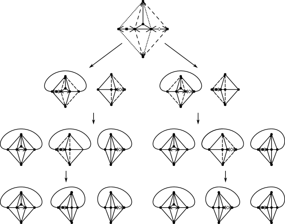
Figure 3. In the topmost figure, the short–dashed circuit is $\delta$ and the long–dashed circuit is $\delta^{\prime}$. After the first splitting, the algorithm says to split successively along the dashed curves in the second and third rows. The bottommost diagrams are graph isomorphic. The Seifert fiber components that are produced are not shown in this figure

The remainder of Figure 3 shows that choice of splitting first along $\delta$ yields the same atoroidal components as first splitting along $\delta^{\prime}$. The reader should note that the Seifert fiber components produced do not agree. $\Box$

4. A decomposition for non–obtuse hyperbolic polyhedra

In this section, we show how to apply the decompositions of Petronio and Bonahon-Siebenmann described in the previous section to decompose a non-obtuse hyperbolic polyhedron into components that remain hyperbolic upon being relabeled by $\pi/2$ and the complement of these components. The complementary pieces will generally be hyperbolic cone manifolds with non–geodesic boundary. These components will be discussed more thoroughly in Section 6.

Suppose that $\mathcal{P}$ is a non–obtuse hyperbolic polyhedron that realizes a labeled abstract polyhedron $(P,\Theta)$. Let $\mathcal{Q}_{\mathcal{P}}$ be the cone manifold obtained by doubling $\mathcal{P}$ along its boundary. In the case where $\mathcal{P}$ is a Coxeter polyhedron, $\mathcal{Q}_{\mathcal{P}}$ is an orbifold with fundamental group equal to the index–$2$ orientation preserving subgroup of the reflection group generated by $\mathcal{P}$. It will be useful to consider the associated compact topological orbifold $\mathcal{Q}_{\mathcal{P}}^{\perp}$ that is obtained from $\mathcal{Q}_{\mathcal{P}}$ by changing all cone angles to $\pi$ and capping off each of the punctures in $S^{3}$ that correspond to degree $4$ ideal vertices with pillowcases and each of the punctures that correspond to degree $3$ ideal vertices with orbifold balls. These pillowcases are then part of the boundary of $\mathcal{Q}_{\mathcal{P}}^{\perp}$. Equivalently one can consider the topological closure of the non–compact orbifold. This procedure is analogous to passing from a finite volume hyperbolic manifold, $M,$ to a compact topological manifold $\overline{M}$ by truncating the cusps or forming the closure of $M$.

4.1. Turnover decomposition

The results in this section are a constructive version of a theorem of Dunbar that imply that a non–obtuse hyperbolic polyhedron may be decomposed along a disjoint union of hyperbolic turnovers into components that contain no nontrivial prismatic $3$-circuits [13]. In the case of hyperbolic polyhedral orbifolds, the collection of turnovers produced by Dunbar’s theorem corresponds to the collection of turnovers that pass through the same edges of $\mathcal{P}$ as the spherical turnovers produced by Theorem 3.1 applied to $\mathcal{Q}_{\mathcal{P}}^{\perp}$.

We generalize our earlier definition of turnovers to allow for cone–manifold type singularities. That is, we define a turnover to be a $2$–dimensional cone manifold obtained by doubling a triangle with angles $\alpha,$ $\beta,$ and $\gamma$ along its boundary. A turnover is hyperbolic, Euclidean, or spherical if $\alpha+\beta+\gamma$ is less than, equal to, or greater than $\pi$, respectively.

For each of turnover $s_{i}$ in the collection $\mathcal{S}$ produced by Theorem 3.1 applied to $\mathcal{Q}_{\mathcal{P}}^{\perp}$, there is an associated turnover $t_{i}$ in $\mathcal{Q}_{\mathcal{P}}$ that intersects the same three edges of the singular locus that $s_{i}$ intersects. The rest of this section will show that the collection of turnovers in $\mathcal{S}$ can be constructed directly from the abstract polyhedron $P$ and that there is a geodesic representative in the isotopy class of each $t_{i}$ associated to an $s_{i}\in\mathcal{S}$.

In the projective model of $\mathbb{H}^{3}$, a geodesic plane is the intersection of the open unit ball with an affine plane in $\mathbb{R}\mathbb{P}^{3}$. Suppose that $v\in\mathbb{R}\mathbb{P}^{3}$ is a point not contained in $\overline{\mathbb{H}}^{3}$. Consider the set of affine lines that pass through $v$ and are tangent to $\partial_{\infty}\mathbb{H}^{3}$. The intersection of this set of lines with the boundary of $\mathbb{H}^{3}$ is a circle. The intersection of the plane containing this circle with $\mathbb{H}^{3}$ is the polar hyperplane of $v$. Any hyperbolic geodesic that extends to a line passing though $v$ is orthogonal to the polar hyperplane of $v$.

The following lemma says that to find embedded turnovers in $\mathcal{Q}_{\mathcal{P}}$, it suffices to find prismatic $3$–circuits in $P$.

Lemma 4.1.

If $\gamma\subset P^{*}$ is a prismatic $3$–circuit, then there exists a unique hyperbolic turnover $t$ embedded in $\mathcal{Q}_{\mathcal{P}}$ that meets the faces of $\mathcal{P}$ through which $\gamma$ passes orthogonally.

Proof.

We will work in the projective model of $\mathbb{H}^{3}$. Consider the three defining planes $\Pi_{1},$ $\Pi_{2}$, and $\Pi_{3}$ in which the faces of $\mathcal{P}$ corresponding to the vertices of $\gamma$ lie. By Andreev’s theorem $\Theta(e_{12})+\Theta(e_{23})+\Theta(e_{13})<\pi$ where $e_{ij}=\Pi_{i}\cap\Pi_{j},$ so $\Pi_{1}\cap\Pi_{2}\cap\Pi_{3}=v$ is a point in $\mathbb{R}\mathbb{P}^{3}\setminus\overline{\mathbb{H}}^{3}$. The polar hyperplane, $\Pi_{v}$, of $v$ is orthogonal to $e_{12},$ $e_{23},$ and $e_{13}$, hence is orthogonal to $\Pi_{1},$ $\Pi_{2}$, and $\Pi_{3}$. Since $\mathcal{P}$ is non–obtuse, the intersection of $\Pi_{v}$ with the three half spaces determined by the $\Pi_{i}$ that contain $\mathcal{P}$ is actually contained in $\mathcal{P}$. Therefore, the double of $\Pi_{v}\cap\mathcal{P}$ is the desired hyperbolic turnover, $t$. $\Box$

Lemma 4.2.

If $\gamma_{1}\neq\gamma_{2}$ are prismatic $3$–circuits, then the associated turnovers $t_{1}$ and $t_{2}$ provided by Lemma 4.1 are disjoint.

Proof.

Suppose for contradiction that $t_{1}\cap t_{2}\neq\emptyset.$ If $t_{1}\cap t_{2}$ is a single point, $p$, then $p$ must lie in an edge of the polyhedron $\mathcal{P}$. By the previous lemma, both $t_{1}$ and $t_{2}$ intersect the $1$–skeleton of the polyhedron orthogonally. Hence the two turnovers actually coincide. The only other possibility is that $t_{1}\cap t_{2}$ is $1$–dimensional. Both turnovers are geodesic, so in $\mathcal{Q}_{\mathcal{P}}$ the intersection is a closed geodesic. This is a contradiction as hyperbolic turnovers contain no closed geodesics. $\Box$

A polyhedron is said to be turnover reduced if every prismatic $3$-circuit is trivial. If $\mathcal{P}$ is a turnover reduced hyperbolic polyhedron, then $\mathcal{Q}_{\mathcal{P}}^{\perp}$ is orbifold irreducible. The following is a corollary of Theorem 3.1 and Lemmas 4.1 and 4.2.

Corollary 4.3.

For any non–obtuse hyperbolic polyhedron $\mathcal{P}$, there exists a finite collection $\mathcal{S}$ of disjoint, embedded, nonparallel turnovers such that the closure of each component of $\mathcal{P}\setminus\mathcal{S}$ is a turnover reduced non–obtuse hyperbolic polyhedron.

4.2. Atoroidal components of quadrilateral decomposition

In this section we show that the components of $\mathcal{P}$ that correspond to atoroidal components of $\mathcal{Q}_{\mathcal{P}}^{\perp}$ coming from the decomposition of Theorem 3.2 have hyperbolic interiors. We first explain more explicitly the connection between the prismatic $4$–circuits produced by Theorem 3.2 and the $2$–suborbifolds along which $\mathcal{Q}_{\mathcal{P}}^{\perp}$ is decomposed.

A incompressible suborbifold of the form $S^{2}(2,2,2,2)$ embedded in $\mathcal{Q}_{\mathcal{P}}^{\perp}$ is a topological sphere embedded in the base space of $\mathcal{Q}_{\mathcal{P}}^{\perp}$ that intersects the singular locus in four edges that form a prismatic $4$–circuit. The singular locus, $\Sigma(\mathcal{Q}_{\mathcal{P}}^{\perp})$, is contained in a $2$–sphere, topologically embedded in the base space. We may assume that $S^{2}(2,2,2,2)$ has been isotoped so that it intersects this $2$–sphere transversely. The $3$–orbifold $\mathcal{Q}_{\mathcal{P}}^{\perp}$ admits an order–two self–homeomorphism that fixes the $2$–sphere in which $\Sigma(\mathcal{Q}_{\mathcal{P}}^{\perp})$ is embedded and swaps the complementary components. Let $\mathcal{P}^{\perp}$ be the quotient of $\mathcal{Q}_{\mathcal{P}}^{\perp}$ by the action of this symmetry. The quotient, $\mathcal{P}^{\perp}$, is a non–orientable $3$–orbifold with boundary consisting of the quadrilaterals that come from the quotient of the bounding pillowcases of $\mathcal{Q}_{\mathcal{P}}^{\perp}$ by the action. The incompressible $S^{2}(2,2,2,2)$ suborbifolds descend to embedded quadrilaterals in $\mathcal{P}^{\perp}$. Theorem 3.2 then leads to a decomposition of $\mathcal{P}^{\perp}$ by quadrilaterals into components that correspond to the atoroidal and Seifert–fibered components of the double cover. The decomposition of $\mathcal{P}^{\perp}$ by quadrilaterals leads to a decomposition of the original hyperbolic polyhedron $\mathcal{P}$ by quadrilaterals. The boundary of a component of the decomposition of $\mathcal{P}^{\perp}$ is the union of the decomposition quadrilaterals that it meets.

The following proposition says that the atoroidal components coming from the quadrilateral decomposition admit hyperbolic structures.

Proposition 4.4.

Let $Q$ be a component of the decomposition of $\mathcal{P}$ corresponding to an atoroidal component of the decomposition of $\mathcal{P}^{\perp}$. Let $R$ be the abstract polyhedron with a quadrilateral or triangular face for each quadrilateral or triangular boundary component of $Q$. Then $(R,\Theta)$ is realizable as a hyperbolic polyhedron where $\Theta$ is the labeling which agrees with the dihedral angles of $\mathcal{P}$ and assigns $\pi/2$ to each of the introduced edges.

Proof.

The proof consists of showing that $(R,\Theta)$ satisfies the conditions of Andreev’s theorem. The link of each introduced vertex will be spherical because each such vertex meets at least two edges with dihedral angle $\pi/2.$

Suppose that the introduction of a quadrilateral face, $q$, created a prismatic $3$–circuit $\gamma$ that passes through edges $e_{1}$ and $e_{2}$ of $q$ along with an edge $e_{3}$ not in $q$. By assumption, $Q$ is turnover–reduced, so $\gamma$ must be parallel to a triangular face. This is a contradiction because in $\mathcal{Q}_{\mathcal{P}}^{\perp},$ the $4$–circuit corresponding to $q$ would not be prismatic.

No prismatic $4$–circuits pass through any of the introduced faces, for this would contradict the fact that $Q$ corresponds to an atoroidal component of the decomposition. $\Box$

We use the following theorem of Agol, Storm, and W. Thurston to show that the procedure in Proposition 4.4 does not increase the volume of the atoroidal components [1].

Theorem 4.5 (Agol–Storm–W. Thurston).

Let $\overline{M}$ be a compact manifold with interior M, a hyperbolic $3$–manifold of finite volume. Let $\overline{\Sigma}$ be an incompressible surface in $\overline{M}$. Then

$$\mathrm{Vol}(M)\geq\frac{1}{2}V_{3}||D(M\setminus\!\!\setminus\Sigma)||,$$

where $D(M\setminus\!\!\setminus\Sigma)$ denotes the double of $M\setminus\!\!\setminus\Sigma$ along $\Sigma$ and $||\cdot||$ denotes the Gromov invariant.

In the case where $\Sigma$ is separating and each component of $M\setminus\!\!\setminus\Sigma$ is hyperbolic, this theorem says that the sum of the volumes of the rehyperbolized components of $M\setminus\!\!\setminus\Sigma$ is no more than the volume of $M$.

The following shows that the volume of an atoroidal component of the Bonahon–Siebenmann decomposition of $\mathcal{Q}_{\mathcal{P}}^{\perp}$ is no less than that of the corresponding component with totally geodesic boundary, as described in Proposition 4.4.

Proposition 4.6.

Let $Q$ be a component of the decomposition of $\mathcal{P}$ corresponding to an atoroidal component of the decomposition of $\mathcal{Q}_{\mathcal{P}}^{\perp}$ and let $\mathcal{R}$ be the realization of $(R,\Theta)$ as described in Proposition 4.4. Then $\mathrm{Vol}(\mathcal{R})\leq\mathrm{Vol}(Q)$.

Proof.

Consider the double, $D(\mathcal{Q}_{Q})$ of the orbifold $\mathcal{Q}_{Q}$ along its boundary. The orbifold, $D(\mathcal{Q}_{Q})$, admits a finite volume hyperbolic structure. By Selberg’s lemma, there exists a finite index manifold cover $M_{Q}$ of $D(\mathcal{Q}_{Q})$. The preimage of $\partial(D(\mathcal{Q}_{Q}))$ in $M_{Q}$ is an incompressible surface $\Sigma$. If the index of the cover is $n$, then $\mathrm{Vol}(M_{Q})=n\mathrm{Vol}(D(\mathcal{Q}_{Q}))=4n\mathrm{Vol}(Q).$ Then Theorem 4.5 implies

$$4n\mathrm{Vol}(Q)=\mathrm{Vol}(M_{Q})\geq\frac{1}{2}V_{3}||D(M\setminus\!\!\setminus\Sigma)||=4n\mathrm{Vol}(\mathcal{R}).$$

$\Box$

5. Deformations of polyhedra and volume change

Suppose that $P$ is an abstract polyhedron with $E$ edges. Labelings of $P$ are given by points in $\mathbb{R}^{E}$. Throughout, we consider only non–obtuse labelings. Define

$$\Omega(P)=\left\{\Theta\in(0,\pi/2]^{E}\,\left|\,\begin{array}[]{c}(P,\Theta)\text{ is realizable as a finite volume}\\ \text{hyperbolic polyhedron}\end{array}\right.\right\}.$$

This set is in one–to–one correspondence with the set of isometry classes of non–obtuse hyperbolic polyhedra of finite volume with $1$–skeleton isomorphic to $P$. For convenience will pass from labelings to polyhedra without comment.

If $\Omega(P)$ is non–empty, Andreev’s theorem implies that the closure of $\Omega(P)$ is a convex polytope in $\mathbb{R}^{E}$. Define $\widehat{\Omega}(P)$ similarly as the set of non–obtuse labelings that yield a hyperbolic polyhedron of finite or infinite volume. Theorem 2.2 implies that the closure of $\widehat{\Omega}(P)$ is also a convex polytope in $\mathbb{R}^{E}$.

Suppose that $\mathcal{P}(\Theta_{0})$ and $\mathcal{P}(\Theta_{1})$ are hyperbolic realizations of labeled abstract polyhedra $(P,\Theta_{0})$ and $(P,\Theta_{1})$. A smooth deformation from $\mathcal{P}(\Theta_{0})$ to $\mathcal{P}(\Theta_{1})$ is a piecewise–smooth map

$$\Phi:[0,1]\longrightarrow\widehat{\Omega}(P)$$

such that $\Phi(0)=\mathcal{P}(\Theta_{0})$ and $\Phi(1)=\mathcal{P}(\Theta_{1}).$ A deformation $\Phi$ is said to be angle–nondecreasing or angle–nonincreasing if the projection to each coordinate of the target space composed with $\Phi$ is a nondecreasing or nonincreasing function, respectively.

The following proposition says that there exists an angle–nondecreasing deformation from any generalized hyperbolic Coxeter polyhedron with no prismatic $3$–circuits to a finite volume hyperbolic polyhedron with all dihedral angles $\pi/2$ or $\pi/3$.

Proposition 5.1.

Suppose $P$ is an abstract polyhedron with at least $6$ faces containing no prismatic $3$–circuits and $\Theta\in\widehat{\Omega}(P)$ is of the form $\Theta(e_{i})=\pi/n_{i},$ where each $n_{i}\geq 2$ is an integer. Then there exists $\Theta^{\prime}\in\Omega(P)$ of the form $\Theta^{\prime}(e_{i})=\pi/m_{i},$ where each $m_{i}\in\{2,3\}$ and $m_{i}\leq n_{i}.$

Proof.

Define $\Theta^{\prime}$ as follows:

(1) $$\Theta^{\prime}(e_{i})=\begin{cases}\pi/n_{i}&\text{if }n_{i}=2\text{ or }3\\ \pi/3&\text{if }n_{i}>3.\end{cases}$$

It suffices to check that $\Theta^{\prime}$ satisfies the conditions Andreev’s theorem (Theorem 2.1). By assumption, conditions (1), (2), (3), (4), and (6) are satisfied. The labeling $\Theta$ satisfies condition (2) of the hyperideal version of Andreev’s theorem (Theorem 2.2), so for any prismatic $4$–circuit formed by edges $e_{p}$, $e_{q}$, $e_{r}$, and $e_{s}$, $\Theta(e_{i})\leq\pi/3$ for at least one $i\in\{p,q,r,s\}$. For such an $i$, $\Theta^{\prime}(e_{i})=\pi/3$. Hence $\Theta^{\prime}(e_{p})+\Theta^{\prime}(e_{q})+\Theta^{\prime}(e_{r})+\Theta^{\prime}(e_{s})<2\pi$, so $\Theta^{\prime}$ satisfies condition (5). The argument is similar to show that $\Theta^{\prime}$ satisfies condition (7). $\Box$

Schläfli’s formula describes how the volume of a polyhedron changes as it is deformed. The following generalization of Schläfli’s formula is due to Milnor. Rivin supplies a proof in [20].

Theorem 5.2 (Schläfli’s formula).

Let $\mathcal{P}$ be a non–obtuse hyperbolic polyhedron with vertices $v_{1},\dots,v_{n},$ where $v_{i}$ is ideal for $i>m.$ Let $H_{m+1},\dots,H_{n}$ be a collection of horospheres such that $H_{i}$ is centered at $v_{i}$. Further if there is an edge $e_{ij}$ between $v_{i}$ and $v_{j}$, then $l_{ij}$ is the distance between $v_{i}$ and $v_{j}$ if $i,j\leq m$, the signed distance between $H_{i}$ and $H_{j}$ (negative if the corresponding horoballs intersect) if $i,j>m$ and the signed distance between $H_{i}$ and $v_{j}$ if $i\leq m$ and $j>m.$ Then

$$d\mathrm{Vol}(\mathcal{P})=-\frac{1}{2}\sum_{\text{edges }e_{ij}}l_{ij}d\theta_{ij},$$

where $\theta_{ij}$ is the dihedral angle along the edge $e_{ij}.$

The perhaps surprising fact that the right–hand side does not depend on the choice of horoballs follows from the fact that the link of an ideal vertex is a Euclidean polygon.

One consequence of Schläfli’s formula is that angle–increasing deformations of polyhedra are volume–decreasing. In particular, it implies that the deformation given in Proposition 5.1 is volume–nonincreasing.

Corollary 5.3.

Suppose that $P$ is an abstract polyhedron with no prismatic $3$–circuits. Let $\Theta,\Theta^{\prime}\in\Omega(P)$ be as in Proposition 5.1. If $\mathcal{P}$ and $\mathcal{P}^{\prime}$ are the hyperbolic realizations of $(P,\Theta)$ and $(P,\Theta^{\prime})$ respectively, then $\mathrm{Vol}(\mathcal{P})\geq\mathrm{Vol}(\mathcal{P}^{\prime})$ with equality if and only if $\Theta=\Theta^{\prime}$.

Proof.

By Theorem 2.1, $\Omega(P)$ is a convex polytope in $\mathbb{R}^{E}$. Hence the line segment

$$s(t)=(1-t)\Theta+t\Theta^{\prime}$$

is contained in $\Omega(P)$. Let $\mathcal{P}_{t}$ be the hyperbolic realization of $(P,s(t))$ for $t\in[0,1]$. By definition of $\Theta^{\prime},$ the labeling $s(t)$ restricted to each edge is nondecreasing in $t$. Schläfli’s formula then implies that $\mathrm{Vol}(\mathcal{P})\geq\mathrm{Vol}(\mathcal{P}^{\prime}).$ Since the volume is nonincreasing along $s(t)$, $\Theta=\Theta^{\prime}$ if and only if $ds=0$, in which case, the volume is constant. $\Box$

We will now describe how to deal with turnover reduced polyhedra, that is, polyhedra in which every prismatic $3$–circuit is trivial. Suppose $\mathcal{P}$ is a generalized hyperbolic polyhedron. Define the truncation of $\mathcal{P}$, denoted $\mathcal{P}^{\vee}$, to be the polyhedron defined by the same planes as $\mathcal{P}$ along with the polar hyperplanes of any hyperideal vertices. If $\mathcal{P}$ has no hyperideal vertices, then $\mathcal{P}^{\vee}=\mathcal{P}$. If $\Theta$ is a labeling of an abstract polyhedron $P$ realized by $(\mathcal{P},\Theta)$, then $P^{\vee}$ has an induced labeling $\Theta^{\vee}$ defined by keeping all edge labels the same and labeling the introduced edges $\pi/2$.

Suppose that $P$ is an abstract polyhedron that contains a prismatic $3$–circuit that is parallel to a triangular face $T$. The extension of $P$, denoted $\widetilde{P}$, is obtained by replacing all triangular faces of $P$ that are parallel to prismatic $3$–circuits by vertices. The three edges that formed the prismatic $3$–circuit in $P$ are incident to the new vertex in $\widetilde{P}$. Geometrically, extension is roughly inverse to truncation. More explicitly, suppose that $\Theta\in\Omega(P)$, $\widetilde{\Theta}$ is the restriction of $\Theta$ to $\widetilde{P}$ and $\mathcal{P}$ and $\widetilde{\mathcal{P}}$ are the hyperbolic realizations of $(P,\Theta)$ and $(\widetilde{P},\widetilde{\Theta})$ respectively. If $\Theta$ assigns $\pi/2$ to each of the edges of a triangular face $T$, then $\mathcal{P}=\widetilde{\mathcal{P}}^{\vee}$. If $\Theta$ assigns an angle of less than $\pi/2$ to any of the edges in $T$, then $\mathcal{P}$ contains a polyhedron $\mathcal{Q}$ that differs from $\mathcal{P}$ by a collection of triangular prisms or tetrahedra such that $\mathcal{Q}=\widetilde{\mathcal{Q}}^{\vee}.$ Note that if a polyhedron has the property that any prismatic $3$–circuit is parallel to a face, then the extension of such a polyhedron has no prismatic $3$–circuits whatsoever.

A deformation with face degenerations is a deformation of a polyhedron in which a face degenerates to a vertex of any type. In the case of a polyhedron with a triangular face that is parallel to a prismatic $3$–circuit, face degeneration occurs as the angle sum along the prismatic $3$–circuit approaches and possibly exceeds $\pi$.

Corollary 5.4.

If $\mathcal{P}$ is a turnover reduced hyperbolic polyhedron realizing $(P,\Theta)$ with $\Theta(e)\leq\pi/3$ for any edge $e$ that is not an edge of a triangular face, then there exists an angle–nondecreasing deformation with face degenerations to a $\pi/3$–equiangular ideal polyhedron $\mathcal{P}^{\prime}$.

Proof.

First note that $\widetilde{\mathcal{P}}^{(1)}$ is graph isomorphic to the graph $P^{\prime}$, obtained from $P$ by replacing all triangular faces that are parallel to prismatic $3$–circuits by vertices. The fact that $\Theta\in\Omega(P)$ implies that $\widetilde{\Theta}\in\widehat{\Omega}(P^{\prime}).$ An application of Proposition 5.1 yields the desired labeling of $P^{\prime}$. $\Box$

A polyhedron is atoroidal if every prismatic $4$–circuit is parallel to a face.

Corollary 5.5.

If $\mathcal{P}$ is a turnover reduced and atoroidal hyperbolic polyhedron realizing $(P,\Theta)$ with $\Theta(e)=\pi/2$ for any edge $e$ that is part of a triangular or rectangular face with all degree $3$ vertices, then there exists an angle–nondecreasing deformation with face degenerations to a right-angled polyhedron $\mathcal{P}^{\prime}$.

Proof.

The argument is similar to the previous corollary. $\Box$

For an abstract polyhedron $P$, define

$$V\colon\widehat{\Omega}(P)\to\mathbb{R}$$

by $V(\mathcal{P},\Theta)=\mathrm{Vol}_{\mathbb{H}^{3}}(\mathcal{P}^{\vee},\Theta^{\vee}).$ A generalization of Milnor’s continuity conjecture by Rivin implies that $V$ is continuous on $\widehat{\Omega}(\mathcal{P})$ [19]. Hence by Schläfli’s formula, the deformations in Corollaries 5.4 and 5.5 are volume nonincreasing.

A proof of the lower bound in Theorem 1.1 follows from Corollary 5.5 and a theorem from [4] that we restate here for convenience:

Theorem 5.6 ([4]).

If $\mathcal{P}$ is a right–angled hyperbolic polyhedron, $N_{\infty}$ ideal vertices and $N_{F}$ finite vertices, then

$$\mathrm{Vol}(\mathcal{P})\geq\frac{4N_{\infty}+N_{F}-8}{32}\cdot V_{8}.$$

The following corollary is a better lower bound than that in Theorem 1.1, that follows by disregarding the contributions of the prismatic $3$-circuits.

Corollary 5.7.

Let $\mathcal{P}$ be a non–obtuse hyperbolic polyhedron containing no prismatic $4$–circuits, $N_{4}$ degree $4$ vertices, $N_{3}$ degree $3$ vertices, and $M_{3}$ prismatic $3$–circuits. Then

$$\mathrm{Vol}(\mathcal{P})>\frac{4N_{4}+(N_{3}+M_{3})-8}{32}\cdot V_{8}.$$

Proof.

If $\mathcal{P}$ contains no prismatic $4$-circuits, then by Corollary 5.5, there exists a volume–decreasing deformation from $\mathcal{P}$ to a right–angled polyhedron with $N_{4}$ degree–$4$ vertices and $N_{3}+M_{3}$ degree $3$ vertices. Theorem 2.4 in [4] gives the conclusion. $\Box$

6. On hyperbolic prisms and their volumes

In this section a lower bound on the volume of a hyperbolic Coxeter prism is produced by exhibiting the minimal volume Coxeter $n$–prism for each $n\geq 5$. This lower bound does not extend to the full non–obtuse case, but provides a lower bound for any non–obtuse prism having no dihedral angles in the interval $(\pi/3,\pi/2)$. The final subsection in this section gives a lower bound on the volume of the components of a hyperbolic Coxeter polyhedron $\mathcal{P}$ that correspond to the Seifert–fibered components coming from the decomposition of $\mathcal{Q}_{\mathcal{P}}^{\perp}$ given by Theorems 3.1 and 3.2. Again, the results of the final subsection extend to the case of non–obtuse prisms with no dihedral angles in the interval $(\pi/3,\pi/2)$.

An $n$–prism is a non–obtuse hyperbolic polyhedron consisting of $2$ disjoint $n$–gon faces and $n$ quadrilateral faces as shown in Figure 4. Label the edges of one of the $n$–gon faces cyclically by $a_{1},a_{2}\dots a_{n}$ and the edges of the other $n$–gon by $b_{1},b_{2}\dots b_{n}$ so that $a_{i}$ and $b_{i}$ are edges of the same quadrilateral face. Label the remaining $n$ edges by $c_{1},c_{2}\dots c_{n}$ so that $c_{i}$ is an edge of the quadrilateral faces containing $a_{i}$ and $a_{i+1}$, where the labeling is taken modulo $n$. See Figure 4. Label the dihedral angles along the edges $a_{i}$, $b_{i}$ and $c_{i}$ by $\alpha_{i}$, $\beta_{i}$ and $\gamma_{i}$, respectively.

2pt $a_{1}$ [br] at 48 130 $a_{2}$ [bl] at 27 91 $a_{3}$ [b] at 84 61 $a_{4}$ [br] at 155 69 $a_{5}$ [l] at 183 111 $a_{6}$ [b] at 128 142 $b_{1}$ [tl] at 54 85 $b_{2}$ [tr] at 24 45 $b_{3}$ [t] at 80 12 $b_{4}$ [tl] at 163 23 $b_{5}$ [tr] at 182 64 $b_{6}$ [t] at 122 93 $c_{1}$ [r] at 14 87 $c_{2}$ [l] at 38 43 $c_{3}$ [r] at 126 32 $c_{4}$ [l] at 194 64 $c_{5}$ [r] at 171 109 $c_{6}$ [l] at 82 122

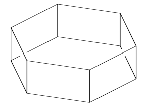
Figure 4. The $1$–skeleton of a hyperbolic $6$–prism

Define $D_{n}$ to be the abstract $n$–prism. By Andreev’s theorem, the space $\Omega(D_{n})$ is naturally parameterized as a convex polytope in $\mathbb{R}^{3n}$ with coordinates given by dihedral angles. Define $O(D_{n})\subset\Omega(D_{n})$ to be the set of labelings of the abstract $n$–prism for which all dihedral angles are of the form $\pi/p$ for $p\in\mathbb{Z}$. The elements of $\mathrm{O}(D_{n})$ are realized by polyhedra that give discrete reflection groups, so correspond to hyperbolic $3$–orbifolds and will be referred to as Coxeter $n$–prisms.

6.1. Basic prisms

Coxeter prisms were described completely by Derevnin and Kim in Theorem 5 of [11]. The following lemma was discovered independently.

Lemma 6.1.

For any prism $\mathcal{D}\in O(D_{n})$, $n\geq 5$, there exists an angle–nondecreasing deformation through prisms $\mathcal{D}_{t}\in\Omega(D_{n})$ with dihedral angles $\alpha_{i}(t),\,\beta_{i}(t),$ and $\gamma_{i}(t)$ from $\mathcal{D}=\mathcal{D}_{0}$ to $\mathcal{D}_{1}\in O(D_{n})$ with dihedral angles satisfying the following properties, up to cyclic permutation of the indices:

1. $\gamma_{1}(1)=\gamma_{2}(1)=\dots=\gamma_{n}(1)=\pi/2$

2. $\alpha_{1}(1)=\beta_{1}(1)=\alpha_{2}(1)=\beta_{2}(1)=\pi/2$

3. For each $i$, $3\leq i\leq n$, $(\alpha_{i}(1),\beta_{i}(1))=(\pi/2,\pi/3)$ or $(\alpha_{i}(1),\beta_{i}(1))=(\pi/3,\pi/2).$

Furthermore, $\mathrm{Vol}(\mathcal{D}_{0})\geq\mathrm{Vol}(\mathcal{D}_{1})$.

Proof.

Let $\mathcal{D}\in O(D_{n})$, $n>4$ with dihedral angles $\alpha_{i},\beta_{i}$, and $\gamma_{i}$ as above. There are no prismatic $3$–circuits in $\mathcal{D}$, so the only restrictions placed on $\mathcal{D}$ by Andreev’s theorem, are that link of each vertex of $\mathcal{D}$ is either a Euclidean or spherical triangle and for each pair $(i,j)$ with $1\leq i\neq j\leq n$ with $i\neq j\pm 1$, modulo $n$, $\alpha_{i}+\alpha_{j}+\beta_{i}+\beta_{j}<2\pi$. Condition (1) of the lemma follows since increasing the $\gamma_{i}$ to $\pi/2$ will increase the angle sum of the link of each vertex, so will satisfy Andreev’s theorem throughout the deformation.

By the fifth condition of Andreev’s theorem, there are at most two pairs $(\alpha_{i},\beta_{i})=(\pi/2,\pi/2)$. If there are two such pairs, they must be adjacent, so without loss of generality, we may assume $(\alpha_{1},\beta_{1})=(\alpha_{2},\beta_{2})=(\pi/2,\pi/2).$ If there is only one such pair, we may assume that it is $(\alpha_{1},\beta_{1})$. Then, $(\alpha_{2},\beta_{2})$ may be deformed to $(\pi/2,\pi/2)$. If there are no such pairs, then $(\alpha_{1},\beta_{1})$ and $(\alpha_{2},\beta_{2})$ may be deformed to $(\pi/2,\pi/2)$. This gives condition (2).

After completing the deformations to satisfy (1) and (2), for each $i=3,\dots n$, at most $1$ of $\alpha_{i}$ and $\beta_{i}$ is $\pi/2$. If one of $\alpha_{i}$ or $\beta_{i}$ is $\pi/2$, then the other is less than or equal to $\pi/3$, so may be increased to $\pi/3$. If neither $\alpha_{i}$ nor $\beta_{i}$ is $\pi/2$, then the pair can be increased to $(\pi/2,\pi/3)$. This yields $\mathcal{D}_{1}$ as described.

The deformations are all angle–increasing, so by Schläfli’s formula, $\mathrm{Vol}(\mathcal{D}_{0})\geq\mathrm{Vol}(\mathcal{D}_{1}).$ $\Box$

An $n$–prism that satisfies the conclusion of Lemma 6.1 will be referred to as a basic $n$–prism. Define an alternating $n$–prism to be a basic $n$–prism for which $\alpha_{3}=\beta_{4}=\alpha_{5}=\dots=\alpha_{n}$ or $\beta_{n}$ if $n$ is odd or even, respectively. Note that for each $n$, there is only one alternating $n$–prism in $O(D_{n})$ up to isometry. It will be shown in Section 6.3 that the alternating $n$–prism is the Coxeter $n$–prism of smallest volume.

6.2. Cubes

In this section, we analyze the geometry of two types of $4$–prisms into which any basic prism may be decomposed. We prove three technical lemmas that will be used to identify the $n$–prism of minimal volume.

For $\mu\in[0,\pi/2)$, define $C_{1}(\mu)$ to be the $4$–prism with $\alpha_{3}=\beta_{4}=\pi/3$, $\gamma_{1}=\mu$, and all other dihedral angles equal to $\pi/2$. A cube such as $C_{1}$ where all dihedral angles are $\pi/2$ except for $\alpha_{3}$, $\beta_{4}$, and $\gamma_{1}$ is known as a Lambert cube. The angles $\alpha_{3}$, $\beta_{4}$, and $\gamma_{1}$ are the essential angles of the Lambert cube. Define $C_{2}(\mu)$ to be the $4$–prism with $\alpha_{3}=\alpha_{4}=\pi/3$, $\gamma_{1}=\mu$, and all other dihedral angles equal to $\pi/2$. For $i=1,2$, let $\rho_{i}(\mu)$ be the hyperbolic length of the edge having dihedral angle $\mu$. See Figure 5. Define $V_{i}(\mu)=\mathrm{Vol}(C_{i}(\mu))$.

2 pt $\frac{\pi}{3}$ [b] at 95 62 $\frac{\pi}{3}$ [tl] at 149 25 $\frac{\pi}{3}$ [b] at 328 62 $\frac{\pi}{3}$ [br] at 378 83 $\rho_{1}(\mu)$ [r] at 3 95 $\rho_{2}(\mu)$ [r] at 235 95 $\mu$ [l] at 26 93 $\mu$ [l] at 258 93 $C_{1}(\mu)$ [t] at 93 -10 $C_{2}(\mu)$ [t] at 331 -10

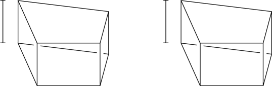
Figure 5. $C_{1}(\mu)$ and $C_{2}(\mu)$

The following lemma shows that $\rho_{i}(\mu)$ is determined by $\mu$.

Lemma 6.2.

Let $\mu\in[0,\pi/2)$. Then,

$$\cosh(\rho_{1}(\mu))=\sqrt{\frac{1+24\cos^{2}{\mu}+\sqrt{1+48\cos^{2}{\mu}}}{32\cos^{2}{\mu}}},$$

and

$$\cosh(\rho_{2}(\mu))=\sqrt{\frac{3\cos{\mu}+1}{4\cos{\mu}}}.$$

Proof.

We will work in the Lobachevsky model of $\mathbb{H}^{3}$ in this proof. Consider the Gram matrix $G(C_{1}(\mu))$ for $C_{1}(\mu)$. Recall that for a polyhedron $\mathcal{P}$,

$$G(\mathcal{P})=\left[w_{i}\cdot w_{j}\right],$$

where $i,\,j\in\{1,\,\dots,\,|\text{Faces}(\mathcal{P})|\}$, $w_{i}$ is the outward unit normal vector to the face $F_{i}$ of $\mathcal{P}$ and the inner product is defined by

(2) $$w_{i}\cdot w_{j}=\begin{cases}1&\text{if }i=j,\\ -\cos{\theta_{ij}}&\text{if }F_{i}\text{ and }F_{j}\text{ meet with dihedral angle }\theta_{ij},\text{ or}\\ -\cosh{d(F_{i},F_{k})}&\text{if }F_{i}\cap F_{j}=\emptyset.\end{cases}$$

Let $F_{1}$ be the face bounded by the edges $a_{i}$, $i=1,\,\dots,\,4$, $F_{2}$ the face bounded by $b_{i}$, $i=1,\,\dots,\,4$, $F_{3}$ and $F_{4}$ the faces containing the edge $c_{1}$, and $F_{5}$ and $F_{6}$ the remaining faces chosen so that $F_{3}\cap F_{5}=\emptyset$ and $F_{4}\cap F_{6}=\emptyset$. Set $x_{1}=-\cosh{d(F_{1},F_{2})},$ $x_{2}=-\cosh{d(F_{3},F_{5})}$, $x_{3}=-\cosh{d(F_{4},F_{6})},$ and $m=-\cos{\mu}$. Note that $x_{1}=-\cosh(\rho_{1}(\mu))$. The Gram matrix for $C_{1}(\mu)$ then is given by

$$G(C_{1}(\mu))=\left[\begin{array}[]{cccccc}1&x_{1}&0&-\frac{1}{2}&0&0\\ x_{1}&1&0&0&-\frac{1}{2}&0\\ 0&0&1&0&x_{2}&m\\ -\frac{1}{2}&0&0&1&0&x_{3}\\ 0&-\frac{1}{2}&x_{2}&0&1&0\\ 0&0&m&x_{3}&0&1\end{array}\right].$$

Since the vectors $w_{i}$ are in $\mathbb{R}^{3,1}$, this matrix can have at most rank $4$. Hence, deleting any row and column leaves a $5$ by $5$ matrix with determinant equal to $0$. Deleting the second row and column gives the equation

$$x_{2}^{2}x_{3}^{2}-x_{2}^{2}-\frac{3}{4}x_{3}^{2}+\frac{3}{4}(1-m^{2})=0.$$

Repeating for the fifth row and column and for the sixth row and column yields

$$x_{1}^{2}x_{3}^{2}+(m^{2}-1)x_{1}^{2}-x_{3}^{2}+\frac{3}{4}(1-m^{2})=0$$

and

$$x_{1}^{2}x_{2}^{2}-x_{1}^{2}-\frac{3}{4}x_{2}^{2}+\frac{9}{16}=0.$$

This system of equations is guaranteed a unique solution with $x_{1},\,x_{2},\,x_{3}<0$ by Andreev’s theorem. A computation shows that there is such a solution with

$$x_{1}=-\sqrt{\frac{24\cos^{2}{\mu}+1+\sqrt{1+48\cos^{2}{\mu}}}{32\cos^{2}{\mu}}},$$

which completes the proof of the first half of the lemma. The second claim of the lemma is proved via identical methods. $\Box$

The next lemma exhibits the relationship between the volume of $C_{1}(\mu)$ and $C_{2}(\mu)$.

Lemma 6.3.

For all $\mu\in[0,\pi/2)$, $V_{1}(\mu)<V_{2}(\mu)$.

Proof.

For $i=1,2$, let $\Phi_{i}:[0,\mu]\to O(D_{4})$ be a smooth deformation from $C_{i}(0)$ to $C_{i}(\mu)$ so that $\gamma_{1}(t)=t$. Then, by Schläfli’s formula,

$$V_{i}(\mu)-V_{i}(0)=-\frac{1}{2}\int_{0}^{\mu}\rho_{i}(t)\,dt,$$

for $i=1,2$. Subtracting $V_{1}(\mu)$ from $V_{2}(\mu)$ gives

$$V_{2}(\mu)-V_{1}(\mu)=(V_{2}(0)-V_{1}(0))+\frac{1}{2}\int_{0}^{\mu}(\rho_{1}(t)-\rho_{2}(t))\,dt.$$

To show that $V_{1}(\mu)<V_{2}(\mu)$, it suffices to show that $V_{1}(0)<V_{2}(0)$ and that $\rho_{2}(t)\leq\rho_{1}(t)$ for all $t\in[0,\mu]$.

If $C$ is a $4$–prism with $0\leq\alpha_{3}<\pi/2$, $0\leq\beta_{4}<\pi/2$, $\gamma_{1}=0$, and all other dihedral angles $\pi/2$, then a special case of a result of Kellerhals in [16] gives

$$\mathrm{Vol}(C)=\frac{1}{4}\bigg{(}\Lambda(\alpha_{3}+\theta)-\Lambda(\alpha_{3}-\theta)+\Lambda(\beta_{4}+\theta)-\Lambda(\beta_{4}-\theta)+4\Lambda\left(\frac{\pi}{2}-\theta\right)\bigg{)},$$

where

$$0<\theta=\arctan{\frac{\sqrt{1-\sin^{2}{\alpha_{3}}\sin^{2}{\beta_{4}}}}{\cos{\alpha_{3}}\cos{\beta_{4}}}},$$

and $\Lambda$ is the Lobachevsky function. Recall that the Lobachevsky function is defined by

$$\Lambda(\theta)=-\int_{0}^{\theta}\log|2\sin t|\,dt.$$

Using this formula, $V_{1}(0)$ can be calculated and is approximately $.44446$.

In the upper half–space model for $\mathbb{H}^{3}$, $C_{2}(0)$ may be obtained by gluing together two copies of the polyhedron bounded by the planes $x=0$, $y=0$, $x=\sqrt{2}/2$, $y=1/2$ and bounded below by the unit hemisphere centered at the origin. By explicitly calculating the integral of the hyperbolic volume form over this polyhedron, it is seen that $V_{2}(0)$ is approximately $.50192$. Hence, $V_{1}(0)<V_{2}(0)$.

Using the formulas derived in Lemma 6.2, a direct calculation shows that $\rho_{1}(t)\geq\rho_{2}(t)$ for all $t\in[0,\pi/2)$, which completes the proof. $\Box$

Finally, we show that the function $V_{1}$ is convex.

Lemma 6.4.

The function $V_{1}(t)=\mathrm{Vol}(C_{1}(t))$ is convex for $t\in[0,\pi/2]$.

Proof.

By the Schläfli differential formula, it suffices to show that

$$\frac{d}{dt}\rho_{1}(t)>0$$

for $t\in[0,\pi/2]$ where

$$\cosh(\rho_{1}(t))=\sqrt{\frac{24\cos^{2}{t}+1+\sqrt{1+48\cos^{2}{t}}}{32\cos^{2}{t}}}.$$

One can check that $\frac{d}{dt}{\cosh^{2}(\rho_{1}(t)})>0$ for $t\in[0,\pi/2]$ by differentiating. Therefore, since $\frac{d}{dx}{x^{2}}>0$ and $\frac{d}{dx}{\cosh(x)}>0$, it follows from the chain rule that $\frac{d}{dt}\rho_{1}(t)>0$ as well. $\Box$

6.3. Alternating prism is minimal volume

In this section, we apply the preceding lemmas to show that the alternating prism is of minimal volume and prove the lower bound in Theorem 1.3.

This lemma describes a decomposition of basic prisms into cubes of the form $C_{1}(\mu)$ and $C_{2}(\nu)$. It is a special case of Theorem 4 in [11] and was independently discovered by the author.

Lemma 6.5.

Suppose that $\mathcal{D}$ is a basic $n$–prism. Then $\mathcal{D}$ can be decomposed into $r$ copies of $C_{1}(\mu)$ and $s=n-r-3$ copies of $C_{2}(\nu)$ where $r\mu+s\nu=\pi/2$.

Proof.

Label the quadrilateral face bounded by $a_{i},b_{i},c_{i},$ and $c_{i-1}$ by $F_{i}$. For each $F_{i}$, $4\leq i\leq n-1,$ there is a unique geodesic plane that contains $c_{1}$ and meets $F_{i}$ orthogonally. Decomposing along these planes gives the desired decomposition into copies of $C_{1}$ and $C_{2}$. The fact that the determining angles of each copy of $C_{i}$, $i=1,2$, are equal follows from the fact that the length of $c_{1}$ determines the dihedral angle $\mu$ by Lemma 6.2. $\Box$

Note that Lemma 6.5 gives a decomposition of the alternating $n$–prism into $n-3$ copies of $C_{1}\left(\frac{\pi}{2(n-3)}\right)$.

Theorem 6.6.

The alternating $n$–prism is the minimal volume prism in $O(D_{n})$.

Proof.

If $\mathcal{D}\in O(D_{n})$ is not a basic prism, then by Lemma 6.1, there is a basic prism with volume smaller than $\mathcal{D}$. Therefore the it suffices to show that the alternating $n$–prism is the smallest volume basic $n$–prism.

By Lemma 6.5, it is enough to show that

$$rV_{1}(\mu)+sV_{2}(\nu)>(r+s)V_{1}\left(\frac{\pi}{2(r+s)}\right),$$

where $r\mu+s\nu=\pi/2$. Setting $t=\frac{r}{r+s}$, the inequality becomes

$$tV_{1}(\mu)+(1-t)V_{2}(\nu)>V_{1}(t\mu+(1-t)\nu).$$

This inequality follows immediately from the fact that $V_{2}>V_{1}$ and the convexity of $V_{1}$. $\Box$

Lemma 6.5 can be used to express the volume of any basic prism in terms of the volume of $C_{1}$ and $C_{2}$. In particular, the volume of the alternating prisms can be calculated explicitly:

Corollary 6.7.

The volume of the alternating $n$–prism $A_{n}$ is given by

$$\mathrm{Vol}(A_{n})=(n-3)\mathrm{Vol}\left(C_{1}\left(\frac{\pi}{2(n-3)}\right)\right).$$

The quantity $\mathrm{Vol}(C_{1}(\frac{\pi}{2(n-3)}))$ can be calculated using a theorem of Kellerhals that we restate here [16]. Suppose that $C$ is a Lambert cube with essential angles $\alpha_{3},$ $\beta_{4}$, and $\gamma_{1}$. The principal parameter, $\theta$, of $C$ is defined by

$$\theta=\arctan{\frac{\sqrt{\cosh^{2}{\rho(\gamma_{1})}-\sin^{2}{\alpha_{3}}\sin^{2}{\beta_{4}}}}{\cos{\alpha_{3}}\cos{\beta_{4}}}},$$

where $\rho(\gamma_{1})$ is the length of the edge $c_{1}$. The volume of the Lambert cube is then given by the following theorem.

Theorem 6.8 (Kellerhals).

Let $C$ be a Lambert cube with essential angles $0\leq\alpha_{3},\,\beta_{4},\,\gamma_{1}\leq\pi/2$. Then the volume of $C$ is given by

$$\mathrm{Vol}(C)=\frac{1}{4}\bigg{(} \Lambda(\alpha_{3}+\theta)-\Lambda(\alpha_{3}-\theta)+\Lambda(\beta_{4}+\theta)-\Lambda(\beta_{4}-\theta)$$

$$+\Lambda(\gamma_{1}+\theta)-\Lambda(\gamma_{1}-\theta)-\Lambda(2\theta)+2\Lambda\left(\frac{\pi}{2}-\theta\right)\bigg{)}.$$

Corollary 6.7 only needs the case where $\alpha_{3}=\beta_{4}=\pi/3$. To find the principal parameter, Lemma 6.2 can be used to compute that

$$\cosh{\rho(\gamma_{1})}=\sqrt{\frac{1+24\cos^{2}{\gamma_{1}}+\sqrt{1+48\cos^{2}{\gamma_{1}}}}{32\cos^{2}{\gamma_{1}}}}.$$

A program such as Mathematica easily computes the volume of Lambert cubes using Kellerhals’ formula.

Finally, it should be noted that for all $n\geq 5$, by Schläfli’s formula

$$\mathrm{Vol}\left(C_{1}\left(\frac{\pi}{2(n-3)}\right)\right)>\mathrm{Vol}\left(C_{1}\left(\frac{\pi}{3}\right)\right)\approx.324423,$$

so we have the following corollary to Corollary 6.7 that bounds the volume of the $n$–prism from below linearly in $n$. This proves the lower bound in Theorem 1.3.

Corollary 6.9.

For any Coxeter $n$–prism $D$,

$$\mathrm{Vol}(D)>(n-3)\cdot\mathrm{Vol}\left(C_{1}\left(\frac{\pi}{3}\right)\right).$$

6.4. Prism regions in non–obtuse polyhedra

For a turnover–reduced non–obtuse polyhedron $\mathcal{P}$, Theorem 3.2 applied to $\mathcal{Q}_{\mathcal{P}}^{\perp}$ gives a collection, $\mathcal{T}$, of topological quadrilaterals along which $\mathcal{P}$ may be decomposed into atoroidal components and prisms. We have already shown how to bound below the volume of the atoroidal components. In this section, we will show how to obtain a lower volume bound on the components of the complement of $\mathcal{T}$ in $\mathcal{P}$ that correspond to the Seifert–fibered components in the splitting of $\mathcal{Q}_{\mathcal{P}}^{\perp}$. We may assume that $\mathcal{P}$ has all dihedral angles equal to $\pi/2$ or $\pi/3$ because by Proposition 5.1, there exists a volume–nonincreasing deformation from any turnover–reduced Coxeter polyhedron to one with all dihedral angles $\pi/2$ or $\pi/3$.

Let $\mathcal{T}^{\prime}\subset\mathcal{T}$ consist of the quadrilaterals in $\mathcal{T}$ that meet both a prism and an atoroidal component of the complement of $\mathcal{T}$. Denote by $\mathcal{P}\setminus\!\!\setminus\mathcal{T}^{\prime}$ the disjoint union of the closures of the components of $\mathcal{P}\setminus\mathcal{T}^{\prime}$. Each component of $\mathcal{P}\setminus\!\!\setminus\mathcal{T}^{\prime}$ is either a collection of atoroidal components glued along $\mathcal{T}\setminus\mathcal{T}^{\prime}$ or a collection of prisms glued along $\mathcal{T}\setminus\mathcal{T}^{\prime}$. Denote the components of $\mathcal{P}\setminus\!\!\setminus\mathcal{T}^{\prime}$ that consist of prisms glued to one another by $\mathcal{G}_{1},\mathcal{G}_{2},\dots\mathcal{G}_{N}$. For each $\mathcal{G}_{i}$, the associated orbifold $\mathcal{Q}_{\mathcal{G}_{i}}^{\perp}$ is a graph orbifold. The boundary of $\mathcal{G}_{i}$, denoted $\partial{G_{i}}$, is $\mathcal{G}_{i}\cap\mathcal{T}^{\prime}$. Each edge of $\mathcal{G}_{i}$ that is intersected by a quadrilateral in $\mathcal{T}\setminus\mathcal{T}^{\prime}$ is a shared edge, in that it is an edge of two prisms that have been glued together. Note that, in general, $\mathcal{G}_{i}$ is not a hyperbolic polyhedron because the boundary of $\mathcal{G}_{i}$ will only be geodesic in special cases. See Figure 6 for an example of a possible $\mathcal{G}_{i}$.

2pt $e_{1}$ [bl] at 261 471 $e_{2}$ [tr] at 290 495 $e_{3}$ [tl] at 290 428 $e_{4}$ [tl] at 260 397

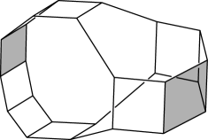
Figure 6. A possible $\mathcal{G}_{i}$. The shaded faces comprise $\partial{\mathcal{G}_{i}}$. The edges $e_{1},$ $e_{2}$, $e_{3}$, and $e_{4}$ are shared edges

To bound the volume from below, we first decompose each $\mathcal{G}_{i}$ further into its constituent prisms by considering the components $\mathcal{D}_{i}^{j}$ of $\mathcal{G}_{i}\setminus\!\!\setminus(\mathcal{T}\setminus\mathcal{T}^{\prime})$. Again, the $\mathcal{D}_{i}^{j}$ are not hyperbolic polyhedra, in general. We label the edges as before, whether or not they are actual geodesic edges as in Figure 7. Label the face bounded by $a_{i},b_{i},c_{i},$ and $c_{i-1}$ by $F_{i}$. The non–geodesic edges will be referred to as virtual edges. The order of $\mathcal{D}_{i}^{j}$ is $n$ if $\mathcal{D}_{i}^{j}$ has $n+2$ total faces, including the non–geodesic faces.

Recall that Lemma 6.1, which follows from Andreev’s theorem, says that there exists a volume–nonincreasing deformation from any Coxeter prism to one where all dihedral angles are $\pi/2$ or $\pi/3$ such that all of the edges $c_{l}$ have dihedral angle $\pi/2$, two adjacent quadrilateral faces have all dihedral angles $\pi/2$ and each other quadrilateral face has exactly one dihedral angle of $\pi/3$. A similar statement is true for the $\mathcal{D}_{i}^{j}$.

2pt $a_{1}$ [br] at 22 84 $a_{2}$ [bl] at 8 56 $a_{3}$ [b] at 47 37 $a_{4}$ [br] at 97 43 $a_{5}$ [l] at 116 71 $a_{6}$ [b] at 77 93 $b_{1}$ [tl] at 27 56 $b_{2}$ [tr] at 7 29 $b_{3}$ [t] at 45 5 $b_{4}$ [tl] at 101 11 $b_{5}$ [tr] at 116 43 $b_{6}$ [t] at 74 62 $c_{1}$ [r] at 0 56 $c_{2}$ [l] at 16 25 $c_{3}$ [r] at 77 17 $c_{4}$ [l] at 122 40 $c_{5}$ [r] at 107 71 $c_{6}$ [l] at 47 81 $\frac{a_{1}}{b_{1}}$ [br] at 191 85 $\frac{a_{2}}{b_{2}}$ [r] at 171 48 $\frac{a_{3}}{b_{3}}$ [tr] at 191 11 $\frac{a_{4}}{b_{4}}$ [tl] at 237 14 $\frac{a_{5}}{b_{5}}$ [l] at 254 47 $\frac{a_{6}}{b_{6}}$ [bl] at 233 85

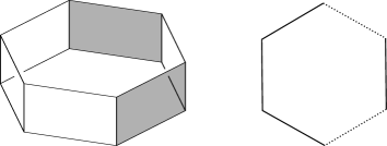
Figure 7. Edge labels for a component $\mathcal{D}_{i}^{j}$ with boundary faces shaded. The figure on the right is a useful schematic for representing such a prism region

Lemma 6.10.

Suppose $\mathcal{P}$ is a hyperbolic Coxeter polyhedron. Then there exists a volume–nonincreasing deformation of $\mathcal{P}$ through hyperbolic polyhedra so that each $\mathcal{D}_{i}^{j}$ in the decomposition described above of the resulting polyhedron has the dihedral angles satisfying the following conditions, up to cyclic relabeling:

1. $\alpha_{1}=\beta_{1}=\pi/2$

2. $\gamma_{k}=\pi/2$ if $c_{k}$ is not a virtual edge.

3. If $a_{2}$ and $b_{2}$ are not virtual edges, then either $(\alpha_{2},\beta_{2})=(\pi/2,\pi/2)$, $(\alpha_{2},\beta_{2})=(\pi/3,\pi/2)$, $(\alpha_{2},\beta_{2})=(\pi/2,\pi/3),$ or $(\alpha_{2},\beta_{2})=(\pi/3,\pi/3).$

4. For each $k$, $3\leq k\leq n$, such that $a_{k}$ and $b_{k}$ are not virtual edges, $(\alpha_{k},\beta_{k})=(\pi/2,\pi/3)$, $(\alpha_{k},\beta_{k})=(\pi/3,\pi/2),$ or $(\alpha_{2},\beta_{2})=(\pi/3,\pi/3).$

Proof.

The proof here is essentially the same as the proof of Lemma 6.1. The first two conditions preclude the existence of any prismatic $4$–circuits passing through all edges with dihedral angles $\pi/2$. By Proposition 5.1, it is certainly the case that all other dihedral angles in each prism region that are less than $\pi/3$ can be deformed to be $\pi/3$. After this deformation, any pair of edges, $(a_{k},b_{k})$, that are not shared edges with $\alpha_{k}=\beta_{k}=\pi/3$ can have either $\alpha_{k}$ or $\beta_{k}$ deformed to $\pi/2$. Figure 8 shows an example where the dihedral angles along a shared edge pair must both remain $\pi/3$. $\Box$

2 pt $\frac{\pi}{2}$ [r] at 0 75 $\frac{\pi}{2}$ [r] at 21 124 $\frac{\pi}{2}$ [l] at 258 68 $\frac{\pi}{2}$ [l] at 278 117 $\frac{\pi}{3}$ [t] at 152 157 $\frac{\pi}{3}$ [t] at 126 103 $\frac{\pi}{2}$ [tl] at 178 19 $\frac{\pi}{2}$ [tl] at 217 89

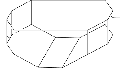
Figure 8. An example where a shared edge pair must both have dihedral angle of $\pi/3$

From now on we will assume that $\mathcal{P}$ satisfies the conclusion of Lemma 6.10. In what follows, we give a decomposition of the prism regions contained in $\mathcal{P}$ and show how this decomposition leads to a lower bound on the volume. The decompositions that follow should be thought of taking place in $\mathcal{P}$ with the previous decomposition into prisms used only as a mental crutch to understand different “regions” within $\mathcal{P}$.

A (topological) quadrilateral $T$ embedded in $\mathcal{P}$ is cylindrical if there exists a prismatic $4$–circuit in $\mathcal{P}\setminus\!\!\setminus T$ that intersects two edges of the boundary component of $\mathcal{P}\setminus\!\!\setminus T$ corresponding to $T$ and two edges with dihedral angle $\pi/2$. See Figure 9. A quadrilateral is acylindrical if it is not cylindrical.

2 pt $T$ [bl] at 151 75 $\frac{\pi}{2}$ [br] at 58 128 $\frac{\pi}{2}$ [br] at 58 46

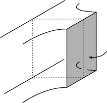
Figure 9. The shaded quadrilateral $T$ is cylindrical

Lemma 6.11.

If $T$ is an acylindrical quadrilateral in a hyperbolic Coxeter polyhedron $\mathcal{P}$, then each component, $\mathcal{P}_{i}$, $i\in\{1,2\}$, of $\mathcal{P}\setminus\!\!\setminus T$ admits a structure as a hyperbolic polyhedron with dihedral angles along the edges of $T\cap\mathcal{P}_{i}$ equal to $\pi/2$. Furthermore,

$$\mathrm{Vol}(\mathcal{P})\geq\mathrm{Vol}(\mathcal{P}_{1})+\mathrm{Vol}(\mathcal{P}_{2}).$$

To prove this lemma, we again apply the theorem of Agol, Storm, and W. Thurston [1].

Proof.

For the first claim, it suffices to show that each $\mathcal{P}_{i}$ satisfies the conditions of Andreev’s theorem (Theorem 2.1) when each of the edges of $T\cap\mathcal{P}_{i}$ are given dihedral angle $\pi/2$. The argument to show this is the same as the argument used to prove Proposition 4.4.

To prove the second claim, we use Theorem 4.5. By Selberg’s Lemma, there exists a $n$–sheeted regular cover $M$ of $\mathbb{H}^{3}/\Gamma(\mathcal{P})$ that is a hyperbolic $3$–manifold [23]. The acylindrical quadrilateral, $T$, lifts to a orientable, incompressible surface $\Sigma$ embedded in $M$. The components, $M_{1}$ and $M_{2}$, of $M\setminus\!\!\setminus\Sigma$ are index $n$ covers of $\mathbb{H}^{3}/\Gamma(\mathcal{P}_{1})$ and $\mathbb{H}^{3}/\Gamma(\mathcal{P}_{2})$ with covering maps induced by the covering map of $M$ to $\mathcal{P}$. Being finite regular covers of hyperbolic orbifolds with geodesic boundary, each of the $M_{i}$ are hyperbolic manifolds with geodesic boundary. Hence, $\mathrm{Vol}(M)=n\mathrm{Vol}(\mathcal{P})$ and $\mathrm{Vol}(M_{i})=n\mathrm{Vol}(\mathcal{P}_{i})$ for $i=1,2$. Then, by Theorem 4.5 and the fact that $\frac{1}{2}V_{3}||D(M_{i})||=\mathrm{Vol}(M_{i})$,

$$n\mathrm{Vol}(\mathcal{P}) =\mathrm{Vol}(M)\geq\frac{1}{2}V_{3}||D({M}\setminus\!\!\setminus\Sigma)||=\frac{1}{2}V_{3}\left(||D(M_{1})||+||D(M_{2})||\right)$$

$$=\mathrm{Vol}(M_{1})+\mathrm{Vol}(M_{2})=n\mathrm{Vol}(\mathcal{P}_{1})+n\mathrm{Vol}(\mathcal{P}_{2}).$$

$\Box$

The following lemma is the basis for the decomposition of the graph orbifold regions that will lead to to the lower bound.

Lemma 6.12.

Let $\mathcal{D}_{i}^{j}$ be a prism region with degree $n\geq 5$.

1. If $\alpha_{1}=\beta_{1}=\alpha_{2}=\beta_{2}=\pi/2$, then for each $k$, $4\leq k\leq n-1$, such that $a_{k}$ and $b_{k}$ are not virtual edges, there exists a geodesic quadrilateral containing $c_{1}$ and intersecting the face $F_{k}$ orthogonally.

2. If $\alpha_{1}=\beta_{1}=\pi/2$ and $\alpha_{2}=\pi/3$ or $\beta_{2}=\pi/3$, then for each $k$, $3\leq k\leq n-1$, there exists an acylindrical quadrilateral that intersects the faces $F_{1}$ and $F_{k}$.

Proof.

1. For each $k\in\{4,\,\dots,\,n-1\}$ such that $a_{k}$ and $b_{k}$ are not virtual edges, let $\Pi_{k}$ be the defining plane of the face of $\mathcal{D}_{i}^{j}$ containing $a_{k}$ and $b_{k}$. Also, let $g_{1}=\Pi_{1}\cap\Pi_{2}$ be the geodesic in which $c_{1}$ is contained. It follows from the fact that $\Pi_{1}$ and $\Pi_{2}$ are disjoint from $\Pi_{k}$ that $g_{1}$ and $\Pi_{k}$ are disjoint. See, for example, Lemma 4.4 of [4]. Hence there exists a geodesic plane, $\Pi,$ that contains $g_{1}$ and intersects $\Pi_{k}$ orthogonally. That $\Pi$ intersects $\mathcal{D}_{i}^{j}$ in a quadrilateral orthogonal to $F_{k}$ is a consequence of the fact that all dihedral angles in $\mathcal{P}$ are no more than $\pi/2$. For the case where $k=4$ or $n-1$ and $a_{k}$ and $b_{k}$ are not virtual, the quadrilaterals coincide with the faces $F_{1}$ and $F_{2}$.

2. Let $k\in\{3,\,\dots,\,n-1\}$. Let $T_{k}$ be a quadrilateral that meets $F_{1}$ and $F_{k}$. If $T_{k}$ were cylindrical, the prismatic $4$–circuit realizing the cylindricity, $\sigma$ must pass through two virtual edges contained of $\mathcal{D}_{i}^{j}$ because for all other pairs of non–virtual edges, $a_{l}$, $b_{l},$ at least one of the dihedral angles is $\pi/3$. Suppose that the two edges of $\sigma$ not in $T_{k}$ are $a$ and $b$. Then there is a prismatic $4$–circuit, $\sigma^{\prime}$, passing through the edges $a$, $b$, $a_{1}$ and $b_{1}$, all of which have dihedral angle $\pi/2$. See Figure 10. This contradicts Andreev’s theorem, so $T_{k}$ must actually be acylindrical.

   2 pt $T_{k}$ [t] at 199 0 $\partial{\mathcal{D}_{i}^{j}}$ [t] at 105 31 $\sigma^{\prime}$ [r] at 0 120 $\sigma$ [r] at 6 129 $a$ [tl] at 8 96 $b$ [tl] at 8 50 $a_{1}$ [t] at 232 73 $b_{1}$ [t] at 232 27

   

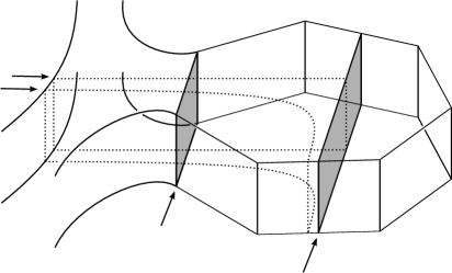
   Figure 10. This illustrates part 2 of the proof of Lemma 6.12

$\Box$

We can now prove the lower bound on the volume of a prism region of $\mathcal{P}$.

Theorem 6.13.

Suppose that $\mathcal{D}_{i}^{j}$ is a prism region of $\mathcal{P}$ that contains $V\geq 2$ vertices of $\mathcal{P}$. Then, except for in the cases shown in Figure 11,

(3) $$\mathrm{Vol}(\mathcal{D}_{i}^{j})>\begin{cases}\left(\frac{V}{2}-3\right)\cdot\mathrm{Vol}\left(C_{1}\left(\lambda\right)\right),&\text{if }V\geq 8\\ C_{1}(\lambda),&\text{if }V=2,\,4\text{ or }6,\end{cases}$$

where $\lambda\in(0,\pi/2)$ depends on $\mathcal{D}_{i}^{j}$. Moreover, if $V\geq 10$, then

$$\mathrm{Vol}(\mathcal{D}_{i}^{j})>\left(\frac{V}{2}-3\right)\cdot\mathrm{Vol}\left(C_{1}\left(\frac{\pi}{3}\right)\right),$$

where the value of $\mathrm{Vol}\left(C_{1}\left(\frac{\pi}{3}\right)\right)$ is approximately $.324423$.

2 pt $\dots$ at 218 92 $\frac{2}{2}$ [tr] at 164 64 $\frac{2}{2}$ [t] at 218 32 $\frac{2}{2}$ [br] at 340 103 $\frac{2}{2}$ [bl] at 404 103 … at 11 43 … at 115 43 $\frac{2}{2}$ [bl] at 96 103 $\dots$ at 374 0

Figure 11. Theorem 6.13 does not provide a lower bound on the volume in these examples. The ellipses may be replaced with any odd number of edges that alternate between dotted and solid and begin with a dotted edge. Recall that these diagrams are explained in Figure 7

Proof.

In each case, we will give a lower bound on the number of cubes of the form $C_{1}$ or $C_{2}$ into which $\mathcal{D}_{i}^{j}$ can be decomposed. The proof finishes in each case by applying the convexity argument used to prove Theorem 6.6.

First suppose that $V\geq 8$, $\alpha_{1}=\alpha_{2}=\beta_{1}=\beta_{2}=\pi/2$, and that $\mathcal{D}_{i}^{j}$ is of order $n$. Lemma 6.12 says that for each $k\in\{4,\,\dots,\,n-1\}$ such that $a_{k}$ and $b_{k}$ are not virtual edges, there exists a geodesic quadrilateral $T_{k}$ that contains $c_{1}$ and intersects $F_{k}$ orthogonally. Since $\mathcal{D}_{i}^{j}$ contains at least $8$ vertices of $\mathcal{P}$, there are at least $V/2-3$ values of $k$, $4\leq k\leq n-1,$ such that $a_{k}$ and $b_{k}$ are not virtual, and such that $a_{k-1}$ and $b_{k-1}$ are not virtual or $a_{k+1}$ and $b_{k+1}$ are not virtual. If $a_{k}$ and $a_{k-1}$ are both not virtual, then just as in the proof of Lemma 6.5, there is a cube $C_{1}(\mu)$ or $C_{2}(\nu)$ formed by $T_{k}$, $T_{k-1}$, $F_{k}$ and $F_{k-1}$, for some $\mu,\,\nu\in(0,\pi/2)$. A similar statement is true if it is $a_{k+1}$ that is not virtual. This procedure gives a cube for each $k\in K$ where

$$K=\{3\leq k\leq n-1\,|\,\text{the endpoints of }c_{k}\text{ are vertices of }\mathcal{P}\}.$$

For each of the at least $V/2-3$ values of $k\in\{4,\dots,n-1\}$ such that $a_{k}$ and $b_{k}$ are not virtual, and such that $a_{k-1}$ and $b_{k-1}$ are not virtual or $a_{k+1}$ and $b_{k+1}$ are not virtual, the endpoints of $c_{k-1}$ or $c_{k}$, respectively, are vertices of $\mathcal{P}$. Therefore $|K|\geq V/2-3$, which completes this case of the proof.

Now suppose that $V\geq 8$ and either $a_{2}$ and $b_{2}$ are virtual, $(\alpha_{2},\beta_{2})=(\pi/2,\pi/3)$, or $(\alpha_{2},\beta_{2})=(\pi/3,\pi/2)$. Choose any value of $k\in\{3,\,\dots,\,n-1\}$ such that $a_{k}$ and $b_{k}$ are not virtual edges and $a_{k-1}$ and $b_{k-1}$ or $a_{k+1}$ and $b_{k+1}$ are virtual edges. Suppose for concreteness that $a_{k-1}$ and $b_{k-1}$ are virtual edges. Then, there exists an acylindrical topological quadrilateral, $T_{k}$, that intersects $F_{1}$ and $F_{k}$ by Lemma 6.12. The prism $\mathcal{D}_{i}^{j}$, as well as the entire polyhedron, $\mathcal{P},$ can be split along this quadrilateral. By Lemma 6.11, each component of $\mathcal{P}\setminus\!\!\setminus T_{k}$ has a hyperbolic structure with $\mathcal{P}\cap T_{k}$ totally geodesic and such that the sum of the volume of the components is no more than the volume of $\mathcal{P}$. The prism region $\mathcal{D}_{i}^{j}$ splits into two prism regions, each of which have a pair of adjacent faces with $\alpha_{i}$ and $\beta_{i}$ equal to $\pi/2$. The decomposition described in the previous case can now be applied to each component. The two resulting components yield the fewest cubes when each of the edges $c_{n-1}$, $c_{n}$, $c_{1}$ and $c_{2}$ are not virtual. In this case, $\mathcal{D}_{i}^{j}$ decomposes into $V/2-2$ cubes.

We now consider the case where $V=2,\,4$ or $6$. The argument is a case–by–case analysis of the possible vertex configurations. We will identify a single cube of the form $C_{1}(\mu)$ or $C_{2}(\mu)$ in each case. The argument then finishes by using the fact that $\mathrm{Vol}(C_{2}(\mu))>\mathrm{Vol}(C_{1}(\mu))$.

Suppose that $V=2$. There are two cases here. First, suppose that $\alpha_{l}=\beta_{l}=\pi/2,$ where the labeling is as in Figure 12. In this case, Lemma 6.12 implies that there exists an acylindrical quadrilateral $T_{1}$. The component of $\mathcal{D}_{i}^{j}\setminus\!\!\setminus T_{1}$ containing the vertices of $\mathcal{P}$ then has volume at least $C_{1}(\mu)$ for some $\mu\in(0,\pi/2)$ by applying the argument from above. In the other case where $\alpha_{1}=\beta_{1}=\pi/2$ or $\alpha_{1}=\beta_{1}=\pi/2$, there is no acylindrical quadrilateral along which to decompose.

2 pt … at 11 43 … at 115 43 $\frac{a_{1}}{b_{1}}$ [bl] at 96 102 $\frac{a_{2}}{b_{2}}$ [br] at 32 102 $\frac{a_{l}}{b_{l}}$ [t] at 64 0

Figure 12. The $2$–vertex case

Next suppose that $V=4$. There are two possible configurations of vertices here. Either the two pairs of vertices of $\mathcal{P}$ are separated by boundary components or they are not. See Figure 13. The previous techniques suffice to find a cube except for in the case where $\alpha_{1}=\beta_{1}=\alpha_{2}=\beta_{2}$ and the vertices are not separated by virtual edges as in the middle diagram of Figure 11, where there is no acylindrical quadrilateral.

2 pt $\dots$ at 64 95 … at 164 71 … at 280 71 $\frac{a_{1}}{b_{1}}$ [tr] at 9 71 $\frac{a_{2}}{b_{2}}$ [t] at 64 46 $\frac{a_{3}}{b_{3}}$ [tl] at 116 71 $\frac{a_{1}}{b_{1}}$ [tr] at 192 17 $\frac{a_{2}}{b_{2}}$ [t] at 253 17 $\frac{a_{l}}{b_{l}}$ [br] at 192 119 $\frac{a_{l+1}}{b_{l+1}}$ [bl] at 253 119

Figure 13. The $4$–vertex case

When $V=6$, there are three possible configurations of vertices. Either none are separated from any other by virtual edges, a single pair is isolated or all three are mutually isolated. See Figure 14. Again the previous methods produce at least one cube in all cases except for the case of the leftmost diagram in Figure 14 where $\alpha_{2}=\beta_{2}=\alpha_{3}=\beta_{3}=\pi/2$ where there is no acylindrical quadrilateral.

2 pt $\dots$ at 63 1 $\dots$ at 166 79 $\dots$ at 284 79 $\dots$ at 334 98 $\dots$ at 442 98 $\dots$ at 387 1 $\frac{a_{1}}{b_{1}}$ [tr] at 10 40 $\frac{a_{2}}{b_{2}}$ [br] at 29 100 $\frac{a_{3}}{b_{3}}$ [bl] at 93 104 $\frac{a_{1}}{b_{1}}$ [tr] at 177 25 $\frac{a_{2}}{b_{2}}$ [t] at 225 1 $\frac{a_{3}}{b_{3}}$ [tl] at 277 26 $\frac{a_{4}}{b_{4}}$ [tl] at 117 39 $\frac{a_{l}}{b_{l}}$ [bl] at 252 119 $\frac{a_{l+1}}{b_{l+1}}$ [br] at 199 119 $c_{l}$ [b] at 226 130 $\frac{a_{1}}{b_{1}}$ [r] at 323 54 $\frac{a_{2}}{b_{2}}$ [tr] at 345 16 $\frac{a_{l}}{b_{l}}$ [tl] at 430 15 $\frac{a_{l+1}}{b_{l+1}}$ [l] at 452 53 $\frac{a_{m}}{b_{m}}$ [bl] at 411 125 $\frac{a_{m+1}}{b_{m+1}}$ [br] at 367 126 $c_{1}$ [r] at 0 77

Figure 14. The $6$–vertex case. The ellipses may be filled in with either a dotted segment or an alternating sequence of dotted and solid segments of odd length beginning with a dotted segment

The second statement follows from the same convexity argument and the fact that for $V\geq 10$, there are at least $2$ cubes in the decomposition. $\Box$

7. Upper bound

The upper bounds in Theorems 1.1 and 1.3 are applications of the upper bounds on the volume of right–angled hyperbolic polyhedra that were proved in [4]:

Theorem 7.1.

([4]) If $\mathcal{P}$ is a $\pi/2$–equiangular hyperbolic polyhedron, $N_{\infty}$ ideal vertices, and $N_{F}\geq 1$ finite vertices, then

$$\mathrm{Vol}(\mathcal{P})<\frac{N_{\infty}-1}{2}\cdot V_{8}+\frac{5N_{F}}{8}\cdot V_{3}.$$

If all vertices of $\mathcal{P}$ are ideal, then

$$\mathrm{Vol}(\mathcal{P})<\frac{N_{\infty}-4}{2}\cdot V_{8}.$$

To apply this theorem, we exhibit a volume–nondecreasing deformation from any given non–obtuse hyperbolic polyhedron to a right–angled polyhedron.

Let $P$ be an abstract polyhedron. Define $\mathcal{N}_{4}(P)$ to be the set of degree $4$ vertices, $\mathcal{N}_{2}(P)$ to be the set of degree $3$ that are adjacent to three vertices of $\mathcal{N}_{4}(P)$, and $\mathcal{N}_{3}(P)$ to be the degree $3$ vertices that are not contained in $\mathcal{N}_{2}(P).$ For $i=2,3,4,$ let $n_{i}(P)=|\mathcal{N}_{i}(P)|$. Define $\mathcal{E}_{33}(P)$ to be the set of edges of $P$ with each endpoint in $\mathcal{N}_{3}(P)$ and $\mathcal{E}_{34}(P)$ to be the set of edges of $P$ with one endpoint in $\mathcal{N}_{3}(P)$ and the other endpoint in $\mathcal{N}_{4}(P)$. Define $E_{ij}(P)=|\mathcal{E}_{ij}(P)|$. Reference to $P$ will be suppressed when the context is clear. An observation that will prove useful is that any edge not in $\mathcal{E}_{33}$ is labeled by $\pi/2$.

The following is the main theorem of this section.

Theorem 7.2.

Let $\mathcal{P}$ be a non–obtuse hyperbolic polyhedron that realizes the labeled abstract polyhedron $(P,\Theta)$. Then

$$\mathrm{Vol}(\mathcal{P})<\frac{n_{4}+E_{33}-1}{2}\cdot V_{8}+\frac{5(E_{34}+n_{2})}{8}\cdot V_{3}.$$

Let $(P,\Theta)$ be a labeled abstract polyhedron. Define the full truncation of $(P,\Theta)$ to be the right–angled abstract polyhedron $\widehat{P}$ obtained by replacing each vertex $v$ in $\mathcal{N}_{3}$ by the triangle formed by the midpoints of the edges entering $v$. Each edge in $\mathcal{E}_{33}$ is collapsed by this procedure. See Figure 15 for an example. In the following lemma, we show that realizability of $(P,\Theta)$ implies realizability of $(\widehat{P},\pi/2)$.

2pt

Figure 15. Full truncation

Lemma 7.3.

If $(P,\Theta)$ is realizable as a hyperbolic polyhedron, then $(\widehat{P},\pi/2)$ is also realizable as a hyperbolic polyhedron.

Proof.

The proof of this lemma amounts to showing that $(\widehat{P},\pi/2)$ satisfies the conditions of Andreev’s theorem restricted to right–angled polyhedra. For an abstract labeled polyhedron $(Q,\pi/2)$, Andreev’s theorem reduces to the following four conditions: $P$ has at least $6$ faces, Each vertex has degree $3$ or degree $4$, $Q$ has no prismatic $4$–circuits, and for any triple of faces $(F_{i},F_{j},F_{k})$ such that $F_{i}\cap F_{j}$ and $F_{j}\cap F_{k}$ are edges with distinct endpoints, $F_{i}\cap F_{k}=\emptyset.$

The number of faces of $\widehat{P}$ is at least the number of faces of $P$. Hence, it is immediate that $\widehat{P}$ has at least $6$ faces unless $P$ has the combinatorial type of a simplex or a triangular prism in which case $\widehat{P}$ has $8$ or $11$ faces, respectively. The fact that all vertices of $\widehat{P}$ are degree $3$ or $4$ is immediate.

Suppose that $\widehat{P}$ contains a triple of faces, $(F_{i},F_{j},F_{k})$ such that $e_{ij}=F_{i}\cap F_{j}$ and $e_{jk}=F_{j}\cap F_{k}$ are edges that have distinct endpoints. We show that $F_{i}\cap F_{k}=\emptyset$ as required by Andreev’s theorem.

Assume for contradiction that $F_{i}\cap F_{k}\neq\emptyset$. If $F_{i}\cap F_{k}$ is an edge, $e_{ik}$, then $e_{ij}$, $e_{jk}$ and $e_{ik}$ would form a prismatic $3$–circuit. The fact that a prismatic $3$–circuit may not pass through a triangular face implies that these three edges correspond to edges in $P$ that are not in $\mathcal{E}_{33}$. Hence in $P$, the corresponding edges form a prismatic $3$–circuit with all three edges labeled by $\pi/2$. This is a contradiction to the assumption that $(P,\Theta)$ satisfies Andreev’s theorem. If $F_{i}\cap F_{k}$ is an ideal vertex $v$, then there are two cases to rule out. The first case is that $F_{i}$ and $F_{k}$ are triangles that arise as degenerations of vertices $v_{1}$ and $v_{2}$ of $P$. Both $v_{1}$ and $v_{2}$ would be vertices of the face corresponding to $F_{j}$ in $P$. This leads to a contradiction, however, for if $v_{1}$ and $v_{2}$ are adjacent in $F_{j}$, they would be vertices of a bigon in $P$, and if $v_{1}$ and $v_{2}$ are non–adjacent vertices of $F_{j}$, there would exist an edge of $P$ connecting two non–adjacent vertices of $F_{j}$. The second case is that $F_{i}$ and $F_{k}$ meet in an ideal vertex and do not arise as degenerations of vertices of $P$. This leads to a contradiction because either the triple of faces in $P$ corresponding to $F_{i},$ $F_{j},$ and $F_{k}$ violate condition (7) of Andreev’s theorem or they form a spherical prismatic $3$–circuit.

Finally, any prismatic $4$–circuit in $\widehat{P}$ cannot pass through any triangular faces. Hence, any edge traversed by a prismatic $4$-circuit in $\widehat{P}$ corresponds to an edge in $P$ that is not in $\mathcal{E}_{33}.$ Andreev’s theorem precludes the existence of any such prismatic $4$-circuits in $P$, which completes the proof. $\Box$

Proof of Theorem 7.2.

For $t\in[0,1)$, let $\Theta_{t}:\text{Edges}(P)\to(0,\pi/2]$ be a labeling of $P$ defined by

(4) $$\Theta_{t}(e)=\begin{cases}(1-t)\Theta(e)&\text{if }e\in E_{33}\\ \Theta(e)=\pi/2&\text{otherwise}.\end{cases}$$

Let $\mathcal{P}_{t}$ be the hyperbolic realization of $(P^{\vee},\Theta^{\vee}_{t})$. Recall from Section 5 that $(P^{\vee},\Theta^{\vee})$ is the labeled abstract polyhedron where all vertices of $P$ around which the angle sum of $\Theta$ is less than $\pi$ are truncated and $\Theta^{\vee}$ agrees with $\Theta$ except along the edges of truncated faces where it assigns $\pi/2$. For $t\in[0,1),$ it is clear that $(P,\Theta_{t})$ satisfies the generalized version of Andreev’s theorem (Theorem 2.2), so $\mathcal{P}_{t}$ satisfies Andreev’s theorem for finite volume hyperbolic polyhedra.

By Schläfli’s formula and Milnor’s continuity conjecture, the function $\mathrm{Vol}(\mathcal{P}_{t})$ is continuous and increasing in $t$. There exists $t_{0}$ so that for all $t>t_{0}$, each vertex in $\mathcal{N}_{3}(P)$ is truncated in $\mathcal{P}_{t}$. For $t>t_{0}$, let $\mathcal{Q}_{t}$ be the hyperbolic cone manifold obtained by doubling $\mathcal{P}_{t}$ along its faces. By the proof of Thurston’s generalized hyperbolic Dehn filling theorem, $\mathcal{Q}_{t}$ converges geometrically to $\widehat{\mathcal{P}}$ doubled along its faces as $t\to 1$ (See, for example, Appendix B of [6]). Therefore, $\mathrm{Vol}(\mathcal{P}_{t})\to\mathrm{Vol}(\widehat{\mathcal{P}}).$ By Lemma 7.3, $\widehat{\mathcal{P}}$ is hyperbolic, so applying Theorem 7.1 to $\widehat{\mathcal{P}}$ completes the proof. $\Box$

The following corollaries give the upper bounds in Theorems 1.1 and 1.3.

Corollary 7.4.

Let $\mathcal{P}$ be a non–obtuse hyperbolic polyhedron containing $N_{4}$ degree $4$ vertices and $N_{3}$ degree $3$ vertices. Then

$$\mathrm{Vol}(\mathcal{P})<\frac{2N_{4}+3N_{3}-2}{4}\cdot V_{8}+\frac{15N_{3}+20N_{4}}{16}\cdot V_{3}.$$

Proof.

Note that $2E_{33}\leq 3n_{3}$, $2E_{34}\leq 3n_{3}+4n_{4}$, $n_{2}+n_{3}=N_{3}$, and $n_{4}=N_{4}$. The corollary then follows from Theorem 7.2 via a simple calculation:

$$\mathrm{Vol}(\mathcal{P}) \leq\frac{n_{4}+E_{33}-1}{2}\cdot V_{8}+\frac{5(E_{34}+n_{2})}{8}\cdot V_{3}$$

$$\leq\frac{2n_{4}+3n_{3}-2}{4}\cdot V_{8}+\frac{5(3n_{3}+4n_{4}+2n_{2})}{16}\cdot V_{3}$$

$$\leq\frac{2N_{4}+3N_{3}-2}{4}\cdot V_{8}+\frac{5(3N_{3}+4N_{4})}{16}\cdot V_{3}.$$

$\Box$

Corollary 7.5.

If $D_{n}$ is an $n$–prism, $n\geq 4$, then

$$\mathrm{Vol}(D_{n})<\frac{3n-4}{2}\cdot V_{8}.$$

Proof.

All edges of an $n$-prism $D_{n}$ are in $\mathcal{E}_{33}$, so $\widehat{D}_{n}$ is a right–angled ideal polyhedron with $E_{33}=3n$ vertices. Apply the ideal case of Theorem 7.1. $\Box$

8. Summary and an example

In this section, we describe how to estimate the volume of any non–obtuse hyperbolic polyhedron $\mathcal{P}$. In all cases, Theorem 7.2 may be used to compute an upper bound for the volume.

In the case where all angles are $\pi/3$ or less, the following theorem follows from the discussion in Section 4.1 and a lower bound on the volume of a $\pi/3$–equiangular polyhedron due to Rivin in a personal communication. A description of his argument is given in [4].

Theorem 8.1.

If $\mathcal{P}$ is a hyperbolic polyhedron with all dihedral angles less than or equal to $\pi/3$, $N\geq 8$ vertices, and $M$ prismatic $3$–circuits, then

$$\mathrm{Vol}(\mathcal{P})>(N+2M)\cdot\frac{3V_{3}}{8}.$$

If $\mathcal{P}$ is an $n$–prism having no dihedral angles in the interval $(\pi/3,\pi/2)$, then Theorem 1.3 says that

$$\mathrm{Vol}(\mathcal{P})>(n-3)\cdot\mathrm{Vol}\left(C_{1}\left(\frac{\pi}{3}\right)\right),$$

where $\mathrm{Vol}(C_{1}(\pi/3))\approx.324423$. If $\mathcal{P}$ is an $n$–prism that does have some dihedral angles in $(\pi/3,\pi/2)$, then the techniques of Section 6 do not hold in their full generality, but may be applied to any sub–cube of $\mathcal{P}$ that has no dihedral angles in $(\pi/3,\pi/2)$.

Otherwise, we first decompose along the collection of triangles and quadrilaterals provided by Theorems 3.1 and 3.2 applied to $\mathcal{Q}_{\mathcal{P}}^{\perp}.$ By Corollary 5.5, each of the resulting atoroidal components may be deformed to right–angled hyperbolic polyhedra with an additional ideal vertex for each quadrilateral face that arose from the Bonahon–Siebenmann decomposition and an additional finite vertex for each triangular face coming from the turnover decomposition. Theorem 5.6 gives a lower bound for each of these components. For each of the prism–type components coming from the Bonahon–Siebenmann decomposition, Theorem 6.13 may be used to obtain a lower bound. In the case that a prism–type component contains dihedral angles in the interval $(\pi/3,\pi/2)$, Theorem 6.13 gives a lower bound for any cube in the decomposition that contains no dihedral angle in $(\pi/3,\pi/2)$.

8.1. An example

We conclude by computing the estimates for an example. The initial polyhedron, $\mathcal{P}$, is displayed on the left in Figure 16. The first step in computing the lower bound is to find a maximal collection of disjoint prismatic $3$–circuits. For this example, there are just two. They are the dashed curves in the diagram on the right in Figure 16.

2pt

$6$ [b] at 85 106

$4$ [r] at 34 30 $2$ [b] at 84 24 $5$ [tr] at 144 16 $4$ [tl] at 29 16 $37$ [br] at 106 259 $2$ [l] at 96 198 $2$ [br] at 70 228 $7$ [l] at 186 272 $2$ [tl] at 130 264 $2$ [bl] at 144 278 $2$ [r] at 140 228 $2$ [r] at 140 214 $2$ [l] at 194 260 $2$ [b] at 83 2

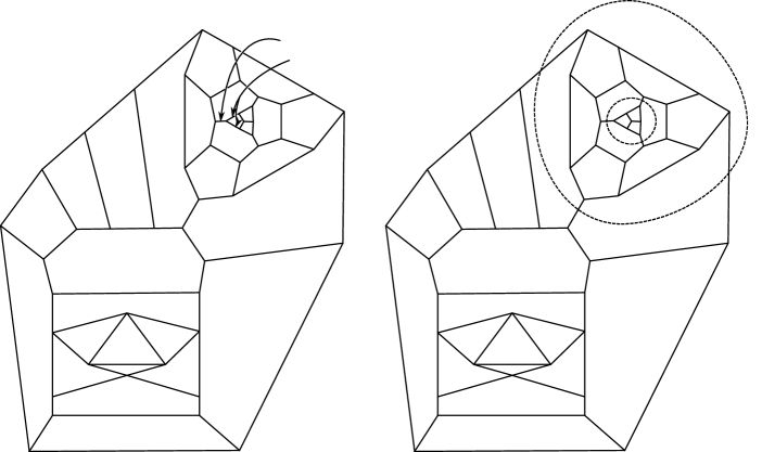
Figure 16. Unlabeled edges that meet a degree four vertex are labeled $2$. Unlabeled edges that meet a degree three vertex but not a degree four vertex are labeled $3$

The polyhedron $\mathcal{P}$ is then decomposed along the corresponding turnovers, as shown in the left–hand diagram in Figure 17. After capping off the turnovers with orbifold balls, the small diagram is seen to be an order $4$ Coxeter prism, so has volume at least $\mathrm{Vol}(C_{1}(\pi/3))\approx.324423$. The other diagram that has been split off can be deformed to a compact right–angled Coxeter polyhedron with $22$ vertices. Therefore these two components contribute at least $\mathrm{Vol}(C_{1}(\pi/3))+\frac{7}{16}\cdot V_{8}$ to the volume of $\mathcal{P}$.

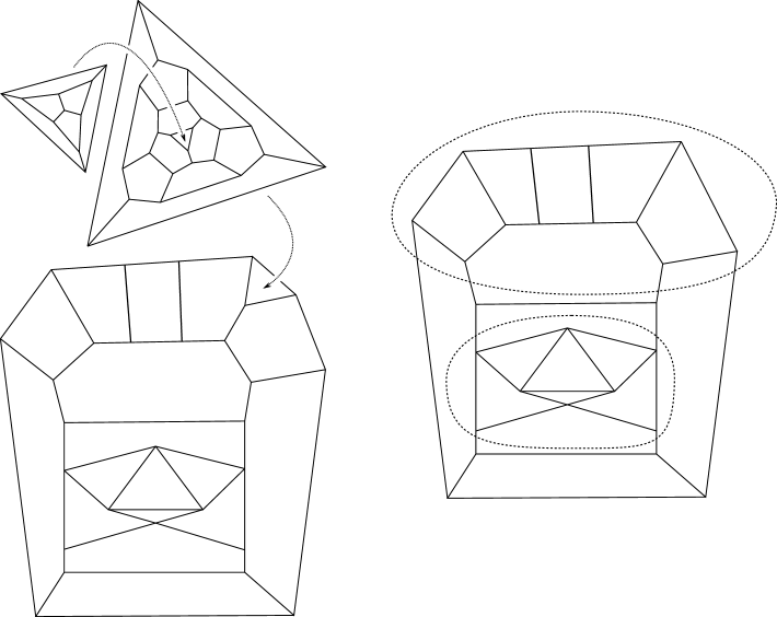
Figure 17. The Coxeter cube is obtained by capping of the bounding triangle on the upper–leftmost diagram. The diagram on the right shows the prismatic $4$–circuits corresponding to the Bonahon–Siebenmann decomposition

The next step is to decompose along a subset of suborbifolds coming from the Bonahon–Siebenmann decomposition into atoroidal and non–atoroidal components. The result of part of this decomposition is seen in the left diagram in Figure 18. The atoroidal component can be deformed to a right–angled polyhedron with $7$ ideal vertices and $2$ finite vertices. Therefore it contributes at least $\frac{25}{16}\cdot V_{8}$ to the volume of $\mathcal{P}$.

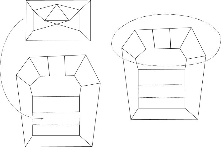
Figure 18. These figures show the decomposition coming from the Bonahon–Siebenmann splitting theorem

Finally, the remaining component, which is a reflection graph orbifold, decomposes into two prism regions. One of these prism regions contains only $6$ vertices of $\mathcal{P}$. Although we know that its volume is at least that of $C_{1}(\mu)$ for some $\mu\in(0,\pi/2)$, we have not shown that $\mu$ is bounded away from $\pi/2$, so the volume of $C_{1}(\mu)$ can be arbitrarily small. The other component has $12$ vertices so contributes at least

$$3\cdot\mathrm{Vol}(C_{1}(\pi/3))$$

to the volume of $\mathcal{P}$.

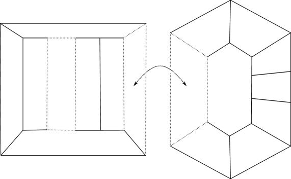
Figure 19. This figure shows the decomposition of the graph orbifold region into two prisms

Adding these lower bounds together gives that the volume of $\mathcal{P}$ is at least $8.625$.

For the upper bound, we use Theorem 7.2. For this example, $n_{2}=0$, $n_{4}=6$, $E_{33}=63$, and $E_{34}=6$. This gives an upper bound of $128.377$.

8.2. Acknowledgements

I wish to thank my thesis advisor, Ian Agol, for many helpful conversations. I also wish to thank Dave Futer, Feng Luo, Shawn Rafalski, and Louis Theran.

References

- [1] Ian Agol, Peter A. Storm, and William P. Thurston. Lower bounds on volumes of hyperbolic Haken 3-manifolds. J. Amer. Math. Soc., 20(4):1053–1077 (electronic), 2007. With an appendix by Nathan Dunfield.
- [2] E. M. Andreev. On convex polyhedra in Lobachevski spaces. Math. USSR Sbornik, 10(3):413–440, 1970.
- [3] E. M. Andreev. On convex polyhedra of finite volume in Lobachevski space. Math. USSR Sbornik, 12(2):255–259, 1970.
- [4] Christopher K. Atkinson. Volume estimates for equiangular hyperbolic Coxeter polyhedra. Algebr. Geom. Topol., 9(2):1225–1254, 2009.
- [5] Xiliang Bao and Francis Bonahon. Hyperideal polyhedra in hyperbolic 3-space. Bull. Soc. Math. France, 130(3):457–491, 2002.
- [6] Michel Boileau and Joan Porti. Geometrization of 3-orbifolds of cyclic type. Astérisque, (272):208, 2001. Appendix A by Michael Heusener and Porti.
- [7] F. Bonahon and L. C. Siebenmann. The characteristic toric splitting of irreducible compact -orbifolds. Math. Ann., 278(1-4):441–479, 1987.
- [8] Yunhi Cho and Hyuk Kim. On the volume formula for hyperbolic tetrahedra. Discrete Comput. Geom., 22(3):347–366, 1999.
- [9] Daryl Cooper, Craig D. Hodgson, and Steven P. Kerckhoff. Three-dimensional Orbifolds and Cone-Manifolds, volume 5 of MSJ Memoirs. Mathematical Society of Japan, 2000.
- [10] William H. Cunningham and Jack Edmonds. A combinatorial decomposition theory. Canad. J. Math., 32(3):734–765, 1980.
- [11] D. A. Derevnin and A. C. Kim. The Coxeter prisms in . In Recent advances in group theory and low-dimensional topology (Pusan, 2000), volume 27 of Res. Exp. Math., pages 35–49. Heldermann, Lemgo, 2003.
- [12] D. A. Derevnin and A. D. Mednykh. A formula for the volume of a hyperbolic tetrahedron. Uspekhi Mat. Nauk, 60(2(362)):159–160, 2005.
- [13] William D. Dunbar. Hierarchies for -orbifolds. Topology Appl., 29(3):267–283, 1988.
- [14] Allen Hatcher. Notes on basic -manifold topology. http://www.math.cornell.edu/ hatcher/3M/3Mdownloads.html.
- [15] Craig D. Hodgson. Deduction of Andreev’s theorem from Rivin’s characterization of convex hyperbolic polyhedra. In Topology ’90 (Columbus, OH, 1990), volume 1 of Ohio State Univ. Math. Res. Inst. Publ., pages 185–193. de Gruyter, Berlin, 1992.
- [16] Ruth Kellerhals. On the volume of hyperbolic polyhedra. Math. Ann., 285:541–569, 1989.
- [17] Jun Murakami and Masakazu Yano. On the volume of a hyperbolic and spherical tetrahedron. Comm. Anal. Geom., 13(2):379–400, 2005.
- [18] Carlo Petronio. Spherical splitting of 3-orbifolds. Math. Proc. Cambridge Philos. Soc., 142(2):269–287, 2007.
- [19] I. Rivin. Continuity of volumes—On a generalization of a conjecture of J. W. Milnor. http://front.math.ucdavis.edu/math.GT/0502543.
- [20] Igor Rivin. Euclidean structures on simplicial surfaces and hyperbolic volume. Ann. of Math. (2), 139(3):553–580, 1994.
- [21] Igor Rivin and Craig D. Hodgson. A characterization of compact convex polyhedra in hyperbolic -space. Invent. Math., 111(1):77–111, 1993.
- [22] Roland K. W. Roeder, John H. Hubbard, and William D. Dunbar. Andreev’s theorem on hyperbolic polyhedra. Ann. Inst. Fourier (Grenoble), 57(3):825–882, 2007.
- [23] Atle Selberg. On discontinuous groups in higher-dimensional symmetric spaces. In Contributions to function theory (internat. Colloq. Function Theory, Bombay, 1960), pages 147–164. Tata Institute of Fundamental Research, Bombay, 1960.
- [24] Daniel D. Sleator, Robert E. Tarjan, and William P. Thurston. Rotation distance, triangulations, and hyperbolic geometry. J. Amer. Math. Soc., 1(3):647–681, 1988.
- [25] E. Steinitz. Polyeder und raumeinteilungen. Enzylk. Math. Wiss., 3:1–139, 1922.
- [26] William Thurston. The geometry and topology of three-manifolds. Lecture notes from Princeton University, 1978-80.
- [27] Akira Ushijima. A volume formula for generalised hyperbolic tetrahedra. In Non-Euclidean geometries, volume 581 of Math. Appl. (N. Y.), pages 249–265. Springer, New York, 2006.
- [28] È. B. Vinberg. The volume of polyhedra on a sphere and in Lobachevsky space. In Algebra and analysis (Kemerovo, 1988), volume 148 of Amer. Math. Soc. Transl. Ser. 2, pages 15–27. Amer. Math. Soc., Providence, RI, 1991.