Optimized Entanglement-Assisted Quantum Error Correction

Abstract

Using convex optimization, we propose entanglement-assisted quantum error correction procedures that are optimized for given noise channels. We demonstrate through numerical examples that such an optimized error correction method achieves higher channel fidelities than existing methods. This improved performance, which leads to perfect error correction for a larger class of error channels, is interpreted in at least some cases by quantum teleportation, but for general channels this interpretation does not hold.

I Introduction

Noise is an important obstacle for the scale-up of quantum information devices—both decoherence due to interactions with an external environment, and the internal control errors inevitable for any information-processing. The theory of quantum error correction was developed by analogy to classical error-correcting codes to overcome this obstacle P.W. Shor (1995); A.M. Steane (1996); Gottesman (1996); E. Knill and R. Laflamme (1997). Quantum error-correcting codes (QECCs) store quantum information redundantly in an entangled state of multiple quantum systems (usually qubits), in such a way that errors can be detected and corrected without directly measuring (and hence disturbing) the quantum information to be protected. The fact that this can be done at all is quite remarkable, and has opened up the prospect that quantum information processing may become a viable technology in the foreseeable future.

Broadly speaking, quantum error correction is useful in two main contexts. The first is quantum computation, where errors that occur during a calculation must be constantly found and corrected to keep them from accumulating. The QECCs used for this purpose must fit into an overall fault-tolerant scheme D. Aharonov and M. Ben-Or (1997); A.Yu. Kitaev (1996); Gottesman (1998); Preskill (1998), which puts important constraints on the properties of the codes used.

The other main context is quantum communication. Here it is assumed that the steps of encoding and decoding are largely error-free, and all errors occurs during the transmission of quantum information through a noisy quantum channel. This is the context we will consider in this paper. It should be noted, though, that this division is not really sharp: quantum computers may well need to transmit information internally, and quantum communication may be part of a distributed information processing scheme.

In the context of quantum communications, one can explore the effect of different shared resources on the ability to detect and correct errors. Recently, a great deal of work has been done on entanglement-assisted quantum error correction (EAQEC), and entanglement-assisted quantum error-correcting codes (EAQECCs). In these schemes, the sender (usually called Alice) and receiver (usually called Bob) share some number of pure maximally-entangled states, or ebits. Alice can use her halves of these ebits in the encoding procedure, and Bob can use his halves in error correction and decoding. The idea of using entanglement to improve error correction was proposed early in the history of quantum information theory Bennett et al. (1996), but it took a long time for the first steps towards designing practical codes Bowen (2002). This work has led to a generalized theory of quantum error correcting codes, the entanglement-assisted stabilizer formalism Brun et al. (2006a, b); Hsieh et al. (2007); Wilde and Brun (2008); Kremsky et al. (2008); Hsieh et al. (2009); Wilde and Brun (2010).

The large majority of work on QECCs has concerned stabilizer codes Gottesman (1996), which can be derived from classical linear codes. In this algebraic approach, one generally tries to design codes that are able to detect and correct an abstract set of errors acting on single qubits, often based on the Pauli operators. QECCs have the property that any linear combination of correctable errors is also a correctable error. Since the Pauli operators form a basis for all single-qubit operators, the ability to correct Pauli-based errors implies the ability to correct more realistic models of noise, provided that errors are not too highly correlated between qubits. The EAQECCs that have mostly been derived so far extend this stabilizer formalism to include a broader class of codes that utilize shared entanglement.

The standard approach to QEC finds encoding and recovery procedures which ensure perfect recovery of quantum states passing through sufficiently weak noisy channels. The disadvantage of this approach is that it may fail when the noise strength, or error probability, is too high. Another approach to QEC is to tailor QECCs to a particular model of realistic noise, derived from a detailed model or from experimental measurements Altepeter et al. (2003); Weinstein et al. (2004); Howard et al. (2006), e.g., via quantum process tomography Chuang and Nielsen (1997); Poyatos et al. (1997); D’Ariano and Presti (2001); Mohseni and Lidar (2006); Emerson et al. (2007); M. Mohseni, A. T. Rezakhani, and D. A. Lidar (2008); Branderhorst et al. (2009). The tailored approach to QEC attempts to find encoding and recovery operations which are optimized relative to the particular experimentally measured noise or assumed noise model, in the sense that they maximize the fidelity (or minimize the distance) of the encoded output state relative to the input state Reimpell and Werner (2005); Yamamoto et al. (2005); Fletcher et al. (2007); Fletcher et al. (2008a, b); Kosut and Lidar (2009); Kosut et al. (2008); Taghavi et al. (2010); Balló and Gurin (2009); Bény and Oreshkov (2010); Ng and Mandayam (2010); Tyson (2009). Both worst case and average case performance has been considered in this setting, which usually involves numerical optimization. The advantage of this approach is that it tends to be more robust to variations in the noise strength than the standard approach Taghavi et al. (2010). Here we further develop the optimized QEC approach by considering, for the first time, entanglement-assisted quantum error correction as an optimization problem.

To formulate the problem for optimization, we break down quantum error correction into three stages. First, the quantum state to be protected is encoded. This procedure appends some number of ancilla qubits in a fixed initial state, and then applies an encoding unitary to the information and ancilla qubits together. These qubits then pass through a noisy channel (assumed to be known). At the receiver’s side, more ancillas can be appended, and then a decoding unitary is applied. All the ancillas (encoding or recovery) are discarded, and the state of the information qubits is the output.

In standard quantum error correction, the encoding and recovery ancillas always start in a standard state (usually $|0\rangle$), and are not entangled with each other. Previous work has shown that regular recovery ancillas are redundant in increasing the error correction fidelity Taghavi et al. (2010). That is, given the same number of information qubits and encoding ancillas, the presence or absence of recovery ancillas makes no difference to the channel fidelity. This matches the properties of stabilizer codes, where decoding can be done unitarily, and there is no benefit in including recovery ancillas.

To formulate the problem for entanglement-assisted codes, we change the initial state of the ancillas, so that noiseless entanglement is shared between the encoding and recovery ancilla qubits. We show that this additional information can enhance the performance of the recovery ancillas, and increase the error correction fidelity in most cases. This initial shared entanglement can in principle improve performance in at least two different ways. It can allow the code to transfer quantum information about the initial state to the recovery block, improving the channel fidelity. This fidelity increase can in fact lead to perfect error correction for an important class of error channels. The error correction procedure for this class of channels can be interpreted as teleportation, with only classical information passing through the noisy channel.

However, even in cases where the error correction protocol is not a form of teleportation, we can still get an improvement in performance. One interpretation of this is that entangled ancillas allow the recovery procedure to extract more information about the errors. This is analogous to superdense coding, where the use of entanglement boosts the rate of classical communication. The fidelity increase here shows the importance of relevant information stored in the ancillas in quantum error correction. The entangled recovery ancillas are fundamentally different than the regular recovery ancillas considered in previous optimization problems, that gave no benefit Taghavi et al. (2010).

The optimization procedure here, similar to previous work in this area Reimpell and Werner (2005); Yamamoto et al. (2005); Fletcher et al. (2007); Fletcher et al. (2008a, b); Kosut and Lidar (2009); Kosut et al. (2008); Taghavi et al. (2010); Balló and Gurin (2009); Bény and Oreshkov (2010); Ng and Mandayam (2010); Tyson (2009), assumes that we know the noise channel. We assume that a channel identification procedure, such as quantum process tomography Altepeter et al. (2003); Weinstein et al. (2004); Howard et al. (2006); Chuang and Nielsen (1997); Poyatos et al. (1997); D’Ariano and Presti (2001); Mohseni and Lidar (2006); Emerson et al. (2007); M. Mohseni, A. T. Rezakhani, and D. A. Lidar (2008); Branderhorst et al. (2009), has been performed prior to the error correction. It is also possible to optimize performance in cases where the exact channel model is not known, though we do not consider that here.

The structure of the paper is as follows. In Section II we formulate the optimization problem in terms of a distance between states that needs to be minimized. The problem is bi-convex in the encoding and recovery operations, and in Sections III and IV we consider how to optimize the encoding for a given recovery, and recovery for a given encoding, respectively. In Section V we consider the case of random unitary channels, and analyze a simple example for which EAQEC has perfect fidelity, via teleportation. We present numerical examples in Section VI, where we contrast different correction and optimization scenarios. These examples illustrate the improved performance of optimized EAQECCs in a setting where perfect fidelity cannot be achieved. We conclude in Section VII. Certain technical details are presented in Appendix A.

II Problem Formulation

A quantum dynamical process is a map from an initial state $\rho$ to a final state $\mathcal{E}(\rho)$. In general the map $\mathcal{E}$ does not represent unitary evolution. However, if we assume a larger closed quantum system that includes the environment (or bath) $B$ of the system, the total evolution becomes unitary. If the initial system-bath state is $\rho_{SB}$, a quantum channel can be written as

$$\mathcal{E}(\rho)=\mathrm{Tr}_{B}[U_{SB}\rho_{SB}U_{SB}^{\dagger}],$$ (1)

where $\rho=\mathrm{Tr}_{B}[\rho_{SB}]$ is the initial system density matrix, $U_{SB}$ is a unitary operator acting on the joint system-bath Hilbert space $\mathcal{H}=\mathcal{H}_{S}\otimes\mathcal{H}_{B}$, $\chi_{B}=\mathrm{Tr}_{S}[\rho_{SB}]$ is the initial state of the environment, and $\mathrm{Tr}_{B}$ ($\mathrm{Tr}_{S}$) denotes the partial trace over the environment (system). In general a quantum dynamical process described by Eq. (1) is a Hermitian map (i.e., it maps Hermitian operators to Hermitian operators) Shabani and Lidar (2009). When the initial system-bath state is purely classicaly correlated (formally, has vanishing quantum discord Ollivier and Zurek (2002)), $\mathcal{E}$ becomes a completely positive (CP), trace-preserving map Rodríguez-Rosario et al. (2008). This condition is also necessary Shabani and Lidar (2009). In this case the evolution can be represented using the Kraus operator sum representation (OSR) Kraus (1983); Nielsen and Chuang (2000); Breuer and Petruccione (2002):

$$\mathcal{E}(\rho)=\sum_{i}K_{i}\rho K_{i}^{\dagger},$$ (2)

where the operators $K_{i}$, known as Kraus operators, satisfy the normalization condition $\sum_{i}K_{i}^{\dagger}K_{i}=I$ (identity). Such maps are powerful tools which can represent different types of noise processes that could be acting on the system.

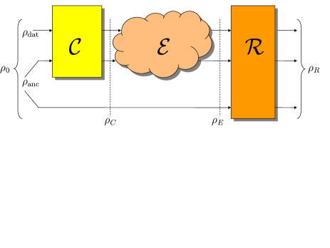
Figure 1: (Color online) Scheme of entanglement-assisted error correction. The data qubits are represented by $\rho_{\rm dat}$. The encoding and recovery ancillas are entangled before the encoding procedure $\mathcal{C}$ begins, and are represented by $\rho_{\rm anc}$. The joint initial system state is $\rho_{0}=\rho_{\rm dat}\otimes\rho_{\rm anc}$. The recovery ancillas pass through a noiseless channel to the recovery operation $\mathcal{R}$. The information qubits and encoding ancillas pass through a noisy channel $\mathcal{E}$. The output of the recovery procedure is $\rho_{R}$. The intermediate states $\rho_{C}$ (output of the encoding) and $\rho_{E}$ (output of the noise channel) are also indicated.

We shall assume that the error correction procedures of encoding and recovery, as well as the noisy channel, can all be described using Kraus operators. The entire procedure on the system can then be represented as

$$\rho_{0}\overset{\mathcal{C}}{\rightarrow}\rho_{C}\overset{\mathcal{E}}{\rightarrow}\rho_{E}\overset{\mathcal{R}}{\rightarrow}\rho_{R},$$ (3)

where $\mathcal{C}$, $\mathcal{E}$, and $\mathcal{R}$ are the encoding, error and recovery operations respectively. The density matrices $\rho_{0}$ through $\rho_{R}$ are the states of the data qubits and the ancillas, i.e., represent the state of the entire system at different points in time. The initial system state $\rho_{0}:\mathcal{H}_{S}\mapsto\mathcal{H}_{S}$, where $\mathcal{H}_{S}$ is the total system Hilbert space, is taken to be a product state between the data qubits, represented by $\rho_{\mathrm{dat}}$, and the ancillas, represented by $\rho_{\mathrm{anc}}$, i.e., $\rho_{0}=\rho_{\mathrm{dat}}\otimes\rho_{\mathrm{anc}}$. Thus $\mathcal{H}_{S}=\mathcal{H}_{\mathrm{dat}}\otimes\mathcal{H}_{\mathrm{anc}}$, where $\mathcal{H}_{\mathrm{dat}}$ and $\mathcal{H}_{\mathrm{anc}}$ are, respectively, the Hilbert space of the data qubits and of the ancillas. The ancilla Hilbert space further decomposes into an encoding subspace $\mathcal{H}_{\mathrm{enc}}$ and a recovery subspace $\mathcal{H}_{\mathrm{rec}}$: $\mathcal{H}_{\mathrm{anc}}=\mathcal{H}_{\mathrm{enc}}\otimes\mathcal{H}_{\mathrm{rec}}$. We write $d=\dim(\mathcal{H}_{S})$ and otherwise denote the respective dimensions of the various subspaces by:

$$d_{X}=\dim(\mathcal{H}_{X}),\quad X\in\{\mathrm{dat},\mathrm{anc},\mathrm{enc},\mathrm{rec}\}.$$ (4)

Note that

$$d=d_{\mathrm{dat}}d_{\mathrm{anc}},\quad d_{\mathrm{anc}}=d_{\mathrm{enc}}d_{\mathrm{rec}}.$$ (5)

For most of our discussion we shall assume that all encoding ancillas are pairwise maximally entangled with recovery ancillas prior to the encoding operation, whence $d_{\mathrm{enc}}=d_{\mathrm{rec}}$, and $\rho_{\mathrm{anc}}=(\left|B\right\rangle\left\langle B\right|)^{\otimes d_{\mathrm{enc}}}$, where $\left|B\right\rangle$ is a maximally entangled state between encoding and recovery ancilla pairs. Nevertheless, for generality we shall leave $d_{\mathrm{enc}}$ and $d_{\mathrm{rec}}$ unless it is necessary to be more specific. Later, in our numerical examples, we shall also consider regular (unentangled) encoding and recovery ancillas.

Using the OSR for each of these operations, the overall evolution is

$$\rho_{R} = \mathcal{R}\circ\mathcal{E}\circ\mathcal{C}(\rho_{0})$$ (6)

$$= \sum_{c,e,r}(R_{r}E_{e}C_{c})\rho_{0}(R_{r}E_{e}C_{c})^{\dagger},$$

where $\{C_{c}\}_{c=1}^{m_{C}}$, $\{E_{e}\}_{e=1}^{m_{E}}$, and $\{R_{r}\}_{r=1}^{m_{R}}$ are the Kraus operators of the encoding, error, and recovery channels, respectively, all satisfying the normalization condition:

$$\sum_{c}C_{c}^{\dagger}C_{c}=\sum_{e}E_{e}^{\dagger}E_{e}=\sum_{r}R_{r}^{\dagger}R_{r}=I.$$ (7)

All the Kraus operators are here represented by square $d\times d$ matrices, i.e., are operators on $\mathcal{H}_{S}$. The number of Kraus operators for each map depends on the implementation and the basis representation, but the number $m_{E}$ of error operators is bounded above by $d^{2}$ Nielsen and Chuang (2000).

We shall assume that the encoding operation $\mathcal{C}$ is unitary, represented by a single unitary (Kraus) operator $C$. The encoded $d$-dimensional state is therefore

$$\rho_{C}=C(\rho_{\mathrm{dat}}\otimes\rho_{\mathrm{anc}})C^{\dagger}.$$ (8)

Since, as illustrated in Figure 1, the encoding does not act on the second half of the entangled pairs (the recovery ancillas), the encoding unitary $C$ should be represented as $C^{\prime}\otimes I_{\mathrm{rec}}$, where $C^{\prime}$ is a $d_{C^{\prime}}\times d_{C^{\prime}}$ matrix, and where $d_{C^{\prime}}=d_{\mathrm{dat}}d_{\mathrm{enc}}=d_{\mathrm{dat}}\sqrt{d_{\mathrm{anc}}}$. We shall write $I_{X}$ to denote the identity operator acting on a subspace $X$, and reserve $I$ for the identity operator on the entire system space $\mathcal{H}_{S}$.

Our goal is to implement a close approximation to a certain desired unitary $L$ on the entire system space. More specifically, the purpose of optimization is to design the encoding $\mathcal{C}$ and recovery $\mathcal{R}$ for a given error channel $\mathcal{E}$ such that the overall map (6) $\rho_{0}\mapsto\rho_{R}$ is as close as possible to some desired unitary $L:\mathcal{H}_{S}\mapsto\mathcal{H}_{S}$. This goal is different from that pursued in earlier optimization papers (e.g., Kosut and Lidar (2009); Kosut et al. (2008); Taghavi et al. (2010)), where the goal was to obtain a good approximation to a unitary $L_{\mathrm{dat}}:\mathcal{H}_{\mathrm{dat}}\mapsto\mathcal{H}_{\mathrm{dat}}$ acting only on the data qubits. Our present goal is general enough to encapsulate state preservation of the data qubits, e.g., by implementing, with as high a fidelity as possible, a unitary which swaps the data qubits into the recovery qubits at the end of the process, while leaving the data and encoding qubits in a new pure state which is tensored with the recovery qubits. Indeed, this is essentially what happens in our teleportation example (Section V).

Channel fidelity or distance are typical measures of performance between two quantum channels Nielsen and Chuang (2000); Gilchrist et al. (2005); Kretschmann and Werner (2004); Reimpell and Werner (2005). The channel fidelity between the error correction operation $\mathcal{REC}$ and the desired unitary operation $L$ is:

$$f=\frac{1}{d_{\mathrm{dat}}^{2}}\sum_{r,e,}\left|\mathrm{Tr}\ L^{\dagger}R_{r}E_{e}C\right|^{2},$$ (9)

We wish to maximize this fidelity, which satisfies $0\leq f\leq 1$. From (Nielsen and Chuang, 2000, Thm.8.2), $f=1$ if and only if there are constants $\mu_{re}$ such that

$$R_{r}E_{e}C=\mu_{re}L,\quad\sum_{r,e}|\mu_{re}|^{2}=1.$$ (10)

As shown in Taghavi et al. (2010), maximizing the fidelity $f$ is equivalent to minimizing the following distance, which is the approach we focus on henceforth:

$$\delta=\sum_{r,e}\left\|R_{r}E_{e}C-\mu_{re}L\right\|^{2},$$ (11)

where $\left\|X\right\|\equiv(\mathrm{Tr}X^{\dagger}X)^{1/2}$ is the Frobenius norm. The minimization must now include the parameters $\{\mu_{re}\}$ as well. Using straightforward matrix manipulations, we can rewrite this distance as

$$\delta(R,C,\Delta)=\left\|RE(I_{m_{E}}\otimes C)-\Delta\otimes L\right\|^{2}$$ (12)

where $\Delta\equiv[\mu_{re}]$ is an $m_{R}\times m_{E}$ rectangular matrix, $E$ is the $d\times m_{E}d$ rectangular error matrix built using the error Kraus operators as horizontally arranged blocks

$$E=[E_{1}...E_{m_{E}}],$$ (13)

and $R$ is the $m_{R}d\times d$ rectangular matrix obtained by vertically stacking the recovery Kraus operators $R_{r}$:

$$R=\left(\begin{array}[]{c}R_{1}\\ \vdots\\ R_{m_{R}}\end{array}\right).$$ (14)

Therefore, we have $\left\|\Delta\right\|^{2}=\mathrm{Tr}\ \Delta^{\dagger}\Delta=\sum_{r,e}\left|\mu_{re}\right|^{2}=1$, and $R^{\dagger}R=\sum_{r}R_{r}^{\dagger}R_{r}=I$.

Our optimization problem can now be summarized as follows:

$$\mathrm{minimize}\,\,\delta(R,C,\Delta)\,\,\mathrm{subject\,\,to\,\,the\,\,constraints}$$

$$R^{{\dagger}}R = I,\;\;C=C^{\prime}\otimes I_{\mathrm{rec}},\ C^{\prime{\dagger}}C^{\prime}=I_{\mathrm{dat},\mathrm{rec}},~{}~{}\left\|\Delta\right\|^{2}=1,$$

where $I_{\mathrm{dat},\mathrm{rec}}$ denotes the identity operator on $\mathcal{H}_{\mathrm{dat}}\otimes\mathcal{H}_{\mathrm{rec}}$. There are three matrices of parameters $(R,C,\Delta)$ in this expression that are to be optimized. As stated, this optimization is not convex. Therefore, as first suggested by Reimpell and Werner Reimpell and Werner (2005), to identify the optimal values of these parameters, we solve this optimization problem iteratively. Starting with an arbitrary initial encoding operation, we first find the optimized recovery operation, which by itself is a convex problem; we then fix the recovery operation obtained in the previous step, and find the optimized encoding operation, which is also a convex problem; and so on, alternately optimizing the recovery and encoding operations until the procedure converges. $\Delta$ is an intermediary matrix of parameters that must also be recalculated at each step. This iteration continues until the distance (11) stops decreasing. The details of the procedure at each step are provided in the next two sections.

The design of the optimized recovery operation at each step is not affected by the extra constraints added by introducing entanglement in the error correction procedure. This is so because optimization of the recovery operation does not depend on the details of the encoding operation. However, the extra constraints play an important role in identifying the optimized encoding operation, which must be of the desired form $C=C^{\prime}\otimes I_{\mathrm{rec}}$.

The encoding ancillas must be initialized in a maximally entangled state—for example, an EPR pair. However, the distance measure defined in (11) is independent of the initial state of the ancilla qubits. To overcome this problem we add an extra step, an entangling operation $U:\mathcal{H}_{S}\mapsto\mathcal{H}_{S}$, to the procedure. The entangling operation does not act on the data qubits, so it can be written as $U=I_{\mathrm{dat}}\otimes U_{\mathrm{anc}}$, where $U_{\mathrm{anc}}:\mathcal{H}_{\mathrm{anc}}\mapsto\mathcal{H}_{\mathrm{anc}}$. By including this entangling operation in the evolution, the ancillas can be assumed to have the initial state $\left|0\right\rangle$.

III Optimized Encoding Operation

The derivation of the optimized encoding operator is similar to what was done previously in Taghavi et al. (2010), but requires including the entangling operator $U$, and a careful consideration of the subspaces involved. Including the entangling operator, the distance measure (11) can be rewritten as

$$\delta(R,C,\Delta) = \left\|RE(I_{m_{E}}\otimes CU)-\Delta\otimes L\right\|^{2}$$

$$= \sum_{r,e}\left\|R_{r}E_{e}CU-\mu_{re}L\right\|^{2}$$

$$= \mathrm{Tr}[I+C^{{\dagger}}C-UL^{{\dagger}}\sum_{r,e}\mu_{re}^{\ast}R_{r}E_{e}C-h.c.],$$

where in the second line we used the relation between Eqs. (11) and (12), and in the third line we used the definition of the Frobenius norm and the normalization conditions (7) and (10).

As a first step we’ll need to find the unconstrained minimum of $\delta(R,C,\Delta)$ with respect to $C$, i.e., we need to find the solution to $\partial\delta/\partial C=0$ without introducing the condition $C^{{\dagger}}C=I$. To this end we note the following matrix differentiation identities, valid for any pair of matrices $A$ and $Z$ with compatible dimensions, with $A$ being independent of the elements of $Z$:

$$\frac{\partial}{\partial Z}\mathrm{Tr}[AZ] = A^{t},\quad\frac{\partial}{\partial Z}\mathrm{Tr}[AZ^{{\dagger}}]=0.$$ (17)

$$\frac{\partial}{\partial Z}\mathrm{Tr}[ZZ^{{\dagger}}] = Z^{\ast},\quad\frac{\partial}{\partial Z}\mathrm{Tr}[AZ^{{\dagger}}Z]=Z^{\ast}A^{t}$$ (18)

$$\frac{\partial}{\partial Z}\mathrm{Tr}[A(Z\otimes I)] = (\mathrm{Tr}_{2}A)^{t},$$ (19)

where in the last identity the partial trace is over the subspace acted on by the identity operator. We prove all these identities in Appendix A.

Therefore, assuming that the recovery operators $R_{r}$ are fixed, we have

$$\frac{\partial\delta}{\partial C}=C^{\ast}-(UL^{{\dagger}}\sum_{r,e}\mu_{re}^{\ast}R_{r}E_{e})^{t},$$ (20)

so that the solution to the unconstrained optimization problem $\frac{\partial\delta}{\partial C}=0$ is

$$\bar{C}=\sum_{r,e}\mu_{re}(R_{r}E_{e})^{{\dagger}}LU^{{\dagger}}.$$ (21)

We wish to impose the additional structure $C=C^{\prime}\otimes I_{\mathrm{rec}}$, i.e., $C^{\prime}=\frac{1}{d_{\mathrm{rec}}}\mathrm{Tr}_{\mathrm{rec}}C$, where the partial trace is over the recovery ancillas. Thus the unconstrained solution over $\mathcal{H}_{\mathrm{dat}}\otimes\mathcal{H}_{\mathrm{enc}}$ becomes

$$\bar{C}^{\prime} = \arg\min_{C^{\prime}}\delta(R,C^{\prime}\otimes I_{\mathrm{rec}},\Delta)$$ (22)

$$= \frac{1}{d_{\mathrm{rec}}}\mathrm{Tr}_{\mathrm{rec}}\left[\sum_{r,e}\mu_{re}(R_{r}E_{e})^{{\dagger}}L(I_{\mathrm{dat}}\otimes U_{a}^{{\dagger}})\right].$$

The reader can check that this result can also be derived by introducing the decomposition $C=C^{\prime}\otimes I_{\mathrm{rec}}$ directly into Eq. (LABEL:del) and using identity (19), i.e.,

$$\frac{\partial\delta}{\partial C^{\prime}}=d_{\mathrm{rec}}C^{\prime\ast}-(\mathrm{Tr}_{\mathrm{rec}}[UL^{{\dagger}}\sum_{r,e}\mu_{re}^{\ast}R_{r}E_{e}])^{t}.$$ (23)

This is important for the next step.

The constrained problem (LABEL:DisOpt) requires that $C^{\prime{\dagger}}C^{\prime}=I_{\mathrm{dat},\mathrm{rec}}$. To solve this problem we form the Lagrangian

$$\mathcal{L}=\delta(R,C^{\prime},\Delta)+\mathrm{Tr}[P(C^{\prime{\dagger}}C^{\prime}-I_{\mathrm{dat},\mathrm{rec}})],$$ (24)

where $P$ is a Hermitian Lagrange multiplier matrix (because the constraint $C^{\prime{\dagger}}C^{\prime}=I_{\mathrm{dat},\mathrm{rec}}$ is Hermitian). Setting $\partial_{C^{\prime}}\mathcal{L}=0$ we find, using Eqs. (18), (22), and (23): $C^{\prime\ast}-\bar{C}^{\prime\ast}+C^{\prime\ast}P^{t}=0$, i.e., the solution to the constrained problem is

$$C^{\prime}=\bar{C}^{\prime}(I_{\mathrm{dat},\mathrm{rec}}+P)^{-1}.$$ (25)

To eliminate $P$ we note that the constraint $C^{\prime{\dagger}}C^{\prime}=I_{\mathrm{dat},\mathrm{rec}}$ now implies $\bar{C}^{\prime{\dagger}}\bar{C}^{\prime}=(I_{\mathrm{dat},\mathrm{rec}}+P)^{2}$, from which we have $(I_{\mathrm{dat},\mathrm{rec}}+P)^{-1}=(\bar{C}^{\prime{\dagger}}\bar{C}^{\prime})^{-1/2}$. Thus, finally

$$C^{\prime}=\bar{C}^{\prime}(\bar{C}^{\prime{\dagger}}\bar{C}^{\prime})^{-1/2},$$ (26)

where $\bar{C}^{\prime}$ is given in Eq. (22). This encoding operation is optimized for the given recovery operation $R$.

IV Optimized Recovery Operation

Unlike the case of the optimized encoding operation, we do not impose any specific tensor product structure on the recovery, so that derivation of the optimized recovery operator is essentially the same as what was done previously in Taghavi et al. (2010), except that again we must include the entangling operator. Here we briefly outline the steps required to optimize the recovery operator. Using the constraints in (LABEL:DisOpt) and fixing the encoding operation $C$, we express the distance (11) as

$$\delta = \left\|RE(I_{m_{E}}\otimes CU)-\Delta\otimes L\right\|^{2}$$ (27)

$$= 2d-2\text{Re}\mathrm{Tr}RE(\Delta^{\dagger}\otimes CUL^{\dagger}).$$

Minimizing (27) with respect to $R$ is the same as maximizing the last term. As shown in (Taghavi et al., 2010, Appendix A) this maximization yields

$$\underset{R^{\dagger}R=I}{\max} \text{Re}\,\mathrm{Tr}\ RE(\Delta^{\dagger}\otimes CUL^{\dagger})$$ (28)

$$= \mathrm{Tr}\sqrt{E(\Gamma\otimes I)E^{\dagger}}$$

where the matrix $\Gamma$ is defined as

$$\Gamma=\Delta^{\dagger}\Delta.$$ (29)

The constraint $\left\|\Delta\right\|^{2}=1$ from (LABEL:DisOpt) is equivalent to $\mathrm{Tr}\ \Gamma=1$, and $\Gamma\geq 0$ by definition. Therefore, the optimization problem for $\Gamma$ is:

$$\mathrm{maximize}\,\,\mathrm{Tr}\sqrt{E(\Gamma\otimes I)E^{{\dagger}}}\,\,\mathrm{subject\,\,to}$$

$$\Gamma \geq 0,\;\;\mathrm{Tr}\Gamma=1.$$ (30)

The optimized $\Gamma$ can be obtained by solving an equivalent semidefinite programming (SDP) problem, or by performing a constrained least squares optimization Taghavi et al. (2010). The matrix $\Delta$ can be obtained from $\Gamma$ by the definition (29) (see Eq. (21) of Ref. Taghavi et al. (2010) for details). Once the optimized $\Delta$ is known, the optimized recovery matrix can be found from

$$R=[v_{1}\ ...\ v_{d}][u_{1}\ ...\ u_{d}]^{\dagger},$$ (31)

where $\{v_{i},u_{i}\}_{i=1}^{d}$ are, respectively, the right and left singular vectors in the singular value decomposition of the matrix $E(\Delta^{\dagger}\otimes CUL^{\dagger})$, with the singular values in descending order.

The algorithm below summarizes the preceding method for encoding and recovery optimization in the presence of entanglement between the encoding and recovery blocks.

Initialize $C$

Repeat

a) Optimal recovery

maximize (30) to find $\Gamma$

solve for $\Delta$ via (29)

solve for $R$ via (31)

b) Optimal encoding

solve for $C$ via (26)

Until distance (11) stops decreasing

Since in each iteration of this algorithm the distance $\delta$ only decreases, the converged solution to this optimization is guaranteed to be at least a locally optimal solution to (LABEL:DisOpt). We apply this procedure to a selection of different channels below to assess its performance in practice.

V Random Unitary Channels

An error channel $\mathcal{E}$ is called a random unitary channel if we can decompose it into the probabilistic application of one of a finite set of unitary operations:

$$\mathcal{E}(\rho)=\underset{i=1}{\overset{n}{\sum}}p_{i}V_{i}\rho V_{i}^{\dagger},$$ (32)

where the $V_{i}$ are unitary operators and $p_{i},i=1,\ldots,n$ is a probability distribution. Random unitary channels describe noise processes that can be corrected using classical information extracted from the environment Gregoratti and Werner (2003). It is clear that any random unitary channel should be unital, meaning that $\mathcal{E(}I)=I$. However, the inverse relation holds only for channels on qubits, and is not true for higher dimensions Tregub (1986); Kümmerer and Maassen (1987).

There are two operations in (1) that are not random unitary. These operations are the introduction of the ancillas and the partial trace over the environment. Therefore, an error channel need not be random unitary, of form (32), in general. The necessary and sufficient conditions for a channel to be a random unitary are discussed in Audenaert and Scheel (2008). In Buscemi (2006), an upper bound was found on the number of unitaries needed in (32). Here we show that if the number of unitary operators required in (32) is at most two, our optimized error correction method can perfectly correct the error using only one EPR pair as ancilla qubits.

In fact, for this case, the optimized encoding and recovery operations are known, and are equivalent to teleportation. To see this, consider a channel that can be decomposed into two unitaries, $V_{1}$ and $V_{2},$ as follows:

$$\mathcal{E}(\rho)=(1-p)V_{1}\rho V_{1}^{\dagger}+pV_{2}\rho V_{2}^{\dagger}.$$ (33)

Suppose Alice wants to send Bob one qubit of data through this noisy channel. One pair of entangled qubits enables Alice and Bob to make this communication error-free. Assume this pair of qubits was prepared by an entanglement source and sent to Alice and Bob, each taking one of the qubits. Alice can apply an encoding operation on her qubits—the data qubit and her half of the ebit—before sending them to Bob through the noisy channel. Bob applies the recovery operation to all three qubits once he receives the message.

Figure 2: Quantum error correction using teleportation. The information qubit $|q_{0}\rangle$ is recovered with unity fidelity in spite of passing through the noise channel $\mathcal{E}$. The first two operations (Hadamard gate on $|q_{1}\rangle$ and controlled-NOT between $|q_{1}\rangle$ and $|q_{2}\rangle$) represent the entangling operation. This is followed by the encoding operation $\mathcal{C}$ described by Eq. (35). The last two operations represent conditional $X$ and $Z$ gates applied to $|q_{2}\rangle$, dependent on the measurement outcomes of $|q_{0}\rangle$ and $|q_{1}\rangle$. See the text for additional details.

The optimized encoding operation that Alice uses in this scenario is done by first applying $V_{1}^{\dagger}$ to her qubits (recall that we assume that the channel is known), to make the error channel equivalent to

$$\mathcal{E}(\rho)=(1-p)I\rho I+pV_{2}V_{1}^{\dagger}\rho V_{1}V_{2}^{\dagger}$$ (34)

Alice continues the encoding operation by applying

$$C = \frac{1}{2}\bigl{(}\left|v_{1}v_{1}\right\rangle\left\langle B_{1}\right|+\left|v_{1}v_{2}\right\rangle\left\langle B_{2}\right|$$ (35)

$$+\left|v_{2}v_{1}\right\rangle\left\langle B_{3}\right|+\left|v_{2}v_{2}\right\rangle\left\langle B_{4}\right|\bigr{)},$$

where $v_{1}$ and $v_{2}$ are the eigenvectors of the unitary $V_{2}V_{1}^{\dagger}$, and $B_{1}$ to $B_{4}$ are an orthonormal basis of maximally entangled states—for example, the Bell states $\left(\left|00\right\rangle\pm\left|11\right\rangle\right)/\sqrt{2}$ and $\left(\left|10\right\rangle\pm\left|01\right\rangle\right)/\sqrt{2}$. This encoding enables us to send two bits of classical information safely through the noisy channel. These two bits of classical information, together with the second half of the ebit, enable us to recover the original state.

To see this in more detail suppose that the initial state of the data qubit is $\left|\phi_{i}\right\rangle=a\left|0\right\rangle+b\left|1\right\rangle$. The state of the entire system after applying the entangling unitary is

$$\left|\psi_{i}\right\rangle=\frac{1}{\sqrt{2}}[a(\left|000\right\rangle+\left|011\right\rangle)+b(\left|100\right\rangle+\left|111\right\rangle)].$$ (36)

After applying the encoding (35) and error map on the first two qubits, the final state of the entire system is

$$\left|\psi_{tot}\right\rangle = \frac{1}{2\sqrt{2}}\bigl{(}\left|v_{1}v_{1}\right\rangle(a\left|0\right\rangle+b\left|1\right\rangle)$$ (37)

$$+\left|v_{1}v_{2}\right\rangle(a\left|0\right\rangle-b\left|1\right\rangle)$$

$$+\left|v_{2}v_{1}\right\rangle(a\left|1\right\rangle+b\left|0\right\rangle)$$

$$+\left|v_{2}v_{2}\right\rangle(a\left|1\right\rangle-b\left|0\right\rangle)\bigr{)}.$$

This is the state of the system once Bob receives it.

At this point, as shown in Figure 2, he can recover the original state $\left|\phi_{i}\right\rangle$ by measuring the state of the first two qubits. Based on the result of the measurement he applies the appropriate Pauli operator to the last qubit, his half of the ebit, to recover the original state. For example, if he measures the first two qubits to be $\left|v_{2}v_{1}\right\rangle$, he should apply $\sigma_{x}$ to the last qubit to recover the original state.

VI Examples

VI.1 The Bit Flip Channel

As an example of a random unitary channel with two unitary operators, we consider the bit flip error channel, or binary symmetric channel, in which bit flip errors occur independently with probability $p$ on each qubit. This channel can be represented as

$$\mathcal{E}(\rho)=(1-p)I\rho I+p\sigma_{x}\rho\sigma_{x},$$ (38)

where henceforth $\sigma_{x},\sigma_{y},\sigma_{z}$ denote the standard $2\times 2$ Pauli matrices. As shown in Figure 3, this error can be corrected using an ebit as the error-correcting resource. The ebit again is shared between the encoding and recovery parts. The encoding acts on the initial data qubit and the first entangled qubit (the encoding qubit). Considering that the error is already in the form (34), we do not need to apply the initial unitary operator here. Therefore, the optimized encoding operator based on (35) is

$$C=\left|++\right\rangle\left\langle B_{1}\right|+\left|+-\right\rangle\left\langle B_{2}\right|+\left|-+\right\rangle\left\langle B_{3}\right|+\left|--\right\rangle\left\langle B_{4}\right|,$$ (39)

where $\left|+\right\rangle=(\left|0\right\rangle+\left|1\right\rangle)/\sqrt{2}$, $\left|-\right\rangle=(\left|0\right\rangle-\left|1\right\rangle)/\sqrt{2}$, and $B_{1}$ to $B_{4}$ form an orthonormal basis of maximally entangled states. The first entangled qubit together with the initial data qubit are corrupted by the bit flip error while the other entangled qubit (the recovery qubit) stays intact. The recovery operation acts on all the qubits, and can reproduce the initial state by measuring the first two qubits as discussed above, followed by a SWAP between the recovery qubit and the data qubit, which perfectly restores the state of the data qubit.

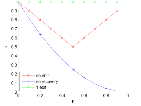
Figure 3: (Color online) Optimized fidelity for the bit flip channel. Results are shown for the case of one data qubit. The blue (bottom) curve is the fidelity without any recovery. The red (middle) curve is the optimized fidelity obtained for encoding using a single encoding qubit but for recovery without entanglement, i.e., with a single recovery qubit in a product state with the encoding qubit. This represents the standard scenario of (channel-optimized) QEC. The green (top) curve is the fidelity obtained in the presence of a single ebit, i.e., the EAQEC scheme shown in Fig. 1. The fidelity in this case is unity for all values of the bit flip probability $p$, showing that our optimization recovers the perfect encoding and recovery protocol of teleportation discussed in the text.

While the optimization procedure we employ is not guaranteed to find the global maximum of the channel fidelity, we see that in this case it does indeed find the optimal solution. Convex optimization has rediscovered the protocol of quantum teleportation.

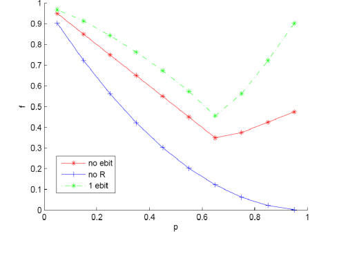
Figure 4: (Color online) Optimized fidelity for the bit-phase flip channel. As in Fig. 3 there is a single data qubit going through the noise channel unprotected (blue, bottom curve), optimally protected by a single encoding and a single recovery qubit in a product state (red, middle curve), and optimally protected by an ebit (green, top curve).

VI.2 The Bit Flip/Phase Flip Channel

In this example both bit flip and phase flip errors occur with equal probabilities:

$$\mathcal{E}(\rho)=(1-p)I\rho I+\frac{p}{2}\sigma_{x}\rho\sigma_{x}+\frac{p}{2}\sigma_{z}\rho\sigma_{z}.$$ (40)

The error occurs independently on different qubits. This error channel clearly cannot be represented in the form of (33). Hence our teleportation argument does not apply here. There is no choice of basis for which classical information can be sent through this channel error-free.

While entanglement cannot enable perfect error correction in this case, it can still increase the useful information about the errors available to the recovery block, and therefore increase the fidelity of the error correction. Figure 4 presents the fidelity of error correction for this channel for different values of $p$. The only difference between the upper and middle curve is the presence of entanglement. Without entanglement, the extra qubit used in the recovery acts as a regular recovery ancilla, and therefore does not increase the fidelity. The minimum fidelity in both cases occurs at $p=2/3$, where the channel is symmetric in $I$, $\sigma_{x}$ and $\sigma_{z}$: $\mathcal{E}(\rho)=(1/3)(I\rho I+\sigma_{x}\rho\sigma_{x}+\sigma_{z}\rho\sigma_{z})$.

Figure 5: (Color online) Optimized fidelity for the depolarizing channel. As in Figs. 3 and 4, there is a single data qubit going through the noise channel unprotected (blue, bottom curve), optimally protected by a single encoding and a single recovery qubit in a product state (blue, middle curve, overlapping red for $p\leq 3/4$), and optimally protected by an ebit (red, top curve).

VI.3 The Depolarizing Channel

In this example we consider a particularly simple error model that is widely used to describe noisy quantum systems: the depolarizing channel. This important channel is often considered to be the quantum equivalent of the binary symmetric channel in classical error correction. It occurs when the state of the system can be completely mixed by the action of the channel. The noise is unbiased in the sense that it generates bit flip errors, phase flip errors, or both with equal probability; this is represented by the map

$$\mathcal{E}(\rho)=(1-p)\rho+\frac{p}{3}\left(\sigma_{x}\rho\sigma_{x}+\sigma_{y}\rho\sigma_{y}+\sigma_{z}\rho\sigma_{z}\right).$$ (41)

The depolarizing channel shrinks the radius of the Bloch sphere by a factor of $1-p,$ while preserving its shape Nielsen and Chuang (2000).

Interestingly, for this error channel the ebit does not increase the fidelity for $p<3/4$. The optimized fidelity of the channel with and without using an ebit is presented in Figure 5. A break point occurs at $p=3/4$, when the coefficients in (41) become equal. The fidelities of both cases are the same for $p<3/4$, but the ebit can slightly increase the fidelity for $p>3/4$.

An observation that may explain this difference is that for $p<3/4$ we can write $\mathcal{E}(\rho)=(1-4p/3)\rho+(4p/3)\mathcal{T}(\rho)$, where $\mathcal{T}$ is the twirling operation:

$$\mathcal{T}(\rho)=\frac{1}{4}\left(\rho+\sigma_{x}\rho\sigma_{x}+\sigma_{y}\rho\sigma_{y}+\sigma_{z}\rho\sigma_{z}\right)=\frac{1}{2}I,$$ (42)

for any valid density matrix $\rho$. In other words, with probability $4p/3$ the channel replaces the qubit with a maximally mixed qubit. For $p>3/4$ this interpretation is no longer possible, and it is in this regime that shared entanglement seems to give improvement.

VII Conclusion

Previous work on optimized quantum error correction Reimpell and Werner (2005); Yamamoto et al. (2005); Fletcher et al. (2007); Fletcher et al. (2008a, b); Kosut and Lidar (2009); Kosut et al. (2008); Taghavi et al. (2010); Balló and Gurin (2009); Bény and Oreshkov (2010); Ng and Mandayam (2010); Tyson (2009). considered the “standard”, entanglement-unassisted setting. In this work we addressed, for the first time, the problem of optimized entanglement-assisted quantum error correction. Our methodology is a generalization of the optimization approach developed in Ref. Taghavi et al. (2010), which involves a bi-convex optimization problem, iterating between encoding and recovery. Our main technical innovation appears in the encoding step, where we introduced a method to account for the constraint of initial entanglement between the encoding and recovery ancillas.

Our method returns the optimized channel fidelity for a given noise channel in the presence of shared entanglement between the encoding and recovery block. We showed that entanglement can substantially increase the error correction fidelity. For specific error channels this fidelity increase can lead to perfect error correction. In these cases, the error correction procedure can be interpreted as quantum teleportation. For cases in which perfect error correction is not possible, this teleportation interpretation does not apply; however, our optimization method returns the optimized fidelity for these channels, in most cases showing improvement with the resource of shared entanglement.

For one channel we found no improvement: the depolarizing channel. For the small codes that we considered in this paper, optimized standard quantum error correction performed just as well as optimized entanglement-assisted quantum error correction on this channel. It is possible that this equivalence between entanglement-assisted and standard quantum error correction will not hold for larger codewords on the depolarizing channel. Larger codewords would use either more ancillas or more ebits in the encoding process. The possibility that larger codes might show a greater difference is suggested by the fact that a three-qubit codeword with two ebits exists that can correct an arbitrary single-qubit error Brun et al. (2006a), while the smallest standard code that corrects an arbitrary error is of size five Laflamme et al. (1996). However, the performance of optimized quantum error correction for larger codewords remains a subject for future research. Larger codewords make for a more numerically intensive optimization procedure.

Considering that regular recovery ancillas are redundant in the optimized error correction procedure, the results of this paper show that information about errors in the encoded data, transferred to the recovery block through entanglement with the encoded state, can increase the fidelity for many channels. We expect that results for a wider variety of error channels and larger codewords will continue to bear this out.

Appendix A Trace differentiation identities

We prove Eqs. (17) and (18). These are one-line proofs which follow directly from the definition of differentiation by a matrix (Bernstein, 2005, Section 10.6): the derivative $\frac{\partial}{\partial Z}f(Z)$ of a differentiable scalar-valued function $f(Z)$ of a matrix argument $Z\equiv[z_{ij}]\in\mathbb{C}^{m\times n}$ is the $m\times n$ matrix whose $(i,j)$ entry is $\frac{\partial}{\partial z_{ij}}f(Z)$:

$$\frac{\partial}{\partial Z}\mathrm{Tr}[AZ] = [\frac{\partial}{\partial z_{ij}}\sum_{ij}z_{ij}a_{ji}]=[a_{ji}]=A^{t},$$ (43)

$$\frac{\partial}{\partial Z}\mathrm{Tr}[AZ^{{\dagger}}] = [\frac{\partial}{\partial z_{ij}}\sum_{ij}a_{ij}z_{ij}^{\ast}]=0,$$ (44)

$$\frac{\partial}{\partial Z}\mathrm{Tr}[ZZ^{{\dagger}}] = [\frac{\partial}{\partial z_{ij}}\sum_{ij}z_{ij}z_{ij}^{\ast}]=[z_{ij}^{\ast}]=Z^{\ast},$$ (45)

$$\frac{\partial}{\partial Z}\mathrm{Tr}[AZ^{{\dagger}}Z] = [\frac{\partial}{\partial z_{ij}}\sum_{ij}z_{ij}(AZ^{{\dagger}})_{ji}]=[(AZ^{{\dagger}})_{ji}]$$ (46)

$$= Z^{\ast}A^{t},$$

where for the second identity we used the fact that for a complex variable $z=x+iy$ ($x,y\in\mathbb{R}$) it holds that $\partial z^{\ast}/\partial z=\partial(x-iy)/\partial x-i\partial(x-iy)/\partial y=0$.

Next we prove Eq. (19). Let

$$A = \sum a_{mnpq}|m\rangle\langle n|\otimes|p\rangle\langle q|,$$ (47)

$$\tilde{Z} = Z\otimes I=\sum z_{m^{\prime}n^{\prime}}|m^{\prime}\rangle\langle n^{\prime}|\otimes|p^{\prime}\rangle\langle p^{\prime}|.$$ (48)

Then

$$\mathrm{Tr}A\tilde{Z} = \mathrm{Tr}\sum a_{mnpp^{\prime}}z_{nn^{\prime}}|m\rangle\langle n^{\prime}|\otimes|p\rangle\langle p^{\prime}|$$ (49)

$$= \sum_{mnp}a_{mnpp}z_{nm},$$

so that

$$\frac{\partial}{\partial Z}\mathrm{Tr}[A(Z\otimes I)] = [\frac{\partial}{\partial z_{mn}}\sum_{mnp}a_{mnpp}z_{nm}]$$ (50)

$$= [\sum_{p}a_{nmpp}]=(\mathrm{Tr}_{2}A)^{t},$$

where the partial trace is over the subspace acted on by the identity operator in $Z\otimes I$.

References

- P.W. Shor (1995) P.W. Shor, Phys. Rev. A 52, R2493 (1995).
- A.M. Steane (1996) A.M. Steane, Phys. Rev. Lett. 77, 793 (1996).
- Gottesman (1996) D. Gottesman, Phys. Rev. A 54, 1862 (1996).
- E. Knill and R. Laflamme (1997) E. Knill and R. Laflamme, Phys. Rev. A 55, 900 (1997).
- D. Aharonov and M. Ben-Or (1997) D. Aharonov and M. Ben-Or, in Proceedings of 29th Annual ACM Symposium on Theory of Computing (STOC) (ACM, New York, NY, 1997), p. 176.
- A.Yu. Kitaev (1996) A.Yu. Kitaev, Russian Math. Surveys 52, 1191 (1996).
- Gottesman (1998) D. Gottesman, Phys. Rev. A 57, 127 (1998).
- Preskill (1998) J. Preskill, Proc. R. Soc. London Ser. A 454, 385 (1998).
- Bennett et al. (1996) C. Bennett, D. DiVincenzo, J. Smolin, and W. Wootters, Phys. Rev. A 54, 3824 (1996).
- Bowen (2002) G. Bowen, Phys. Rev. A 66, 052313 (2002).
- Brun et al. (2006a) T. Brun, I. Devetak, and M.-H. Hsieh, Science 314, 436 (2006a).
- Brun et al. (2006b) T. Brun, I. Devetak, and M.-H. Hsieh (2006b), eprint quant-ph/0608027.
- Hsieh et al. (2007) M.-H. Hsieh, I. Devetak, and T. Brun, Phys. Rev. A 76, 062313 (2007).
- Wilde and Brun (2008) M. Wilde and T. Brun, Phys. Rev. A 77, 064302 (2008).
- Kremsky et al. (2008) I. Kremsky, M.-H. Hsieh, and T. Brun, Phys. Rev. A 78, 012341 (2008).
- Hsieh et al. (2009) M.-H. Hsieh, I. Devetak, and T. Brun, Phys. Rev. A 79, 032340 (2009).
- Wilde and Brun (2010) M. Wilde and T. Brun, Phys. Rev. A 81, 042333 (2010).
- Altepeter et al. (2003) J. B. Altepeter, D. Branning, E. Jeffrey, T. C. Wei, P. G. Kwiat, R. T. Thew, J. L. O’Brien, M. A. Nielsen, and A. G. White, Phys. Rev. Lett. 90, 193601 (2003).
- Weinstein et al. (2004) Y. Weinstein, T. Havel, J. Emerson, N. Boulant, M. Saraceno, S. Lloyd, and D. Cory, J. Chem. Phys. 121, 6117 (2004).
- Howard et al. (2006) M. Howard, J. Twamley, C. Wittman, T. Gaebel, F. Jelezko, and J. Wrachtrup, New J. Phys. 8, 33 (2006).
- Chuang and Nielsen (1997) I. Chuang and M. Nielsen, J. Mod. Optics 44, 2455 (1997).
- Poyatos et al. (1997) J. Poyatos, J. Cirac, and P. Zoller, Phys. Rev. Lett. 78, 390 (1997).
- D’Ariano and Presti (2001) G. M. D’Ariano and P. L. Presti, Phys. Rev. Lett. 86, 4195 (2001).
- Mohseni and Lidar (2006) M. Mohseni and D. A. Lidar, Phys. Rev. Lett. 97, 170501 (2006).
- Emerson et al. (2007) J. Emerson, M. Silva, O. Moussa, C. Ryan, M. Laforest, J. Baugh, D. G. Cory, and R. Laflamme, Science 317, 1893 (2007).
- M. Mohseni, A. T. Rezakhani, and D. A. Lidar (2008) M. Mohseni, A. T. Rezakhani, and D. A. Lidar, Phys. Rev. A 77, 032322 (2008).
- Branderhorst et al. (2009) M. Branderhorst, J. Nunn, I. Walmsley, and R. Kosut, New J. Phys. 11, 115010 (2009).
- Reimpell and Werner (2005) M. Reimpell and R. F. Werner, Phys. Rev. Lett. 94, 080501 (2005).
- Yamamoto et al. (2005) N. Yamamoto, S. Hara, and K. Tsumura, Phys. Rev. A 71, 022322 (2005).
- Fletcher et al. (2007) A. S. Fletcher, P. W. Shor, and M. Z. Win, Phys. Rev. A 75, 012338 (2007).
- Fletcher et al. (2008a) A. Fletcher, P. Shor, and M. Win, IEEE Trans. Inf. Theory 54, 5705 (2008a).
- Fletcher et al. (2008b) A. S. Fletcher, P. W. Shor, and M. Z. Win, Phys. Rev. A 77, 012320 (2008b).
- Kosut and Lidar (2009) R. Kosut and D. A. Lidar, Quant. Inf. Proc. 8, 441 (2009).
- Kosut et al. (2008) R. Kosut, A. Shabani, and D. A. Lidar, Phys. Rev. Lett. 100, 020502 (2008).
- Taghavi et al. (2010) S. Taghavi, R. L. Kosut, and D. A. Lidar, IEEE Trans. Inf. Theory 56, 1461 (2010).
- Balló and Gurin (2009) G. Balló and P. Gurin, Phys. Rev. A 80, 012326 (2009).
- Bény and Oreshkov (2010) C. Bény and O. Oreshkov, Phys. Rev. Lett. 104, 120501 (2010).
- Ng and Mandayam (2010) H. K. Ng and P. Mandayam, Phys. Rev. A 81, 062342 (2010).
- Tyson (2009) J. Tyson (2009), eprint arXiv:0907.3386.
- Shabani and Lidar (2009) A. Shabani and D. A. Lidar, Phys. Rev. Lett. 102, 100402 (2009).
- Ollivier and Zurek (2002) H. Ollivier and W. Zurek, Phys. Rev. Lett. 88, 017901 (2002).
- Rodríguez-Rosario et al. (2008) C. Rodríguez-Rosario, K. Modi, A.-M. Kuah, E. Sudarshan, and A. Shaji, J. Phys. A 41, 205301 (2008).
- Kraus (1983) K. Kraus, States, Effects and Operations, Fundamental Notions of Quantum Theory (Academic, Berlin, 1983).
- Nielsen and Chuang (2000) M. Nielsen and I. Chuang, Quantum Computation and Quantum Information (Cambridge University Press, Cambridge, England, 2000).
- Breuer and Petruccione (2002) H.-P. Breuer and F. Petruccione, The Theory of Open Quantum Systems (Oxford University Press, Oxford, 2002).
- Gilchrist et al. (2005) A. Gilchrist, N. K. Langford, and M. A. Nielsen, Phys. Rev. A 71, 062310 (2005).
- Kretschmann and Werner (2004) D. Kretschmann and R. F. Werner, New J. Phys. 6, 26 (2004).
- Gregoratti and Werner (2003) M. Gregoratti and R. Werner, J. Mod. Optics 50, 915 (2003).
- Tregub (1986) S. L. Tregub, Sov. Math. 30, 105 (1986).
- Kümmerer and Maassen (1987) B. Kümmerer and H. Maassen, Commun. Math. Phys. 109, 1 (1987).
- Audenaert and Scheel (2008) K. M. R. Audenaert and S. Scheel, New J. Phys. 10, 023011 (2008).
- Buscemi (2006) F. Buscemi, Phys. Lett. A 360, 256 (2006).
- Laflamme et al. (1996) R. Laflamme, C. Miquel, J. Paz, and W. Zurek, Phys. Rev. Lett. 77, 198 (1996).
- Bernstein (2005) D. S. Bernstein, Matrix Mathematics (Princeton University Press, Princeton, 2005).