Efficient multiple time scale molecular dynamics: using colored noise thermostats to stabilize resonances

Abstract

Multiple time scale molecular dynamics enhances computational efficiency by updating slow motions less frequently than fast motions. However, in practice the largest outer time step possible is limited not by the physical forces but by resonances between the fast and slow modes. In this paper we show that this problem can be alleviated by using a simple colored noise thermostatting scheme which selectively targets the high frequency modes in the system. For two sample problems, flexible water and solvated alanine dipeptide, we demonstrate that this allows the use of large outer time steps while still obtaining accurate sampling and minimizing the perturbation of the dynamics. Furthermore, this approach is shown to be comparable to constraining fast motions, thus providing an alternative to molecular dynamics with constraints.

I Introduction

Over the past two decades atomistic simulation of chemical, material and biological systems has become a routine and important tool for understanding, analyzing and predicting experiment. Time scales of interest now often span into the microsecond range so as to monitor processes such as protein folding and transport through membranes. However, the shortest atomic time scales in these systems, typically for bonded interactions such as stretches and bends, are of the scale of femtoseconds and therefore time steps of this order are required to stably evolve the system. As a result, billions of steps are needed to reach the time scales of interest, making such simulations a formidable challenge.

Chemical systems typically involve interactions occurring on many time scales ranging from rapidly varying, but cheap to calculate, bonded interactions to slow, but expensive, long range electrostatics. Multiple time scale methods can be used to exploit this separation in time scales by updating the slow interactions less frequently than the fast interactions, in principle allowing significant computational savings to be achieved. Streett et al. (1978); Tuckerman et al. (1990); Grubmuller et al. (1991); Tuckerman et al. (1992) However, the maximum outer time step which can be obtained is in practice limited by the resonance between the slow and fast modes. Biesaideki and Skeel (1993); Ma et al. (2003) This results in energy building up in the high frequency modes, raising the temperature of the system and leading to unstable trajectories and incorrect sampling. As a result the fastest mode in the system still dictates how frequently the slowest interactions must be calculated, thereby limiting the maximum obtainable speed-up. Izaguirre et al. (1999); Zhou et al. (2001)

A commonly used approach to delay the resonance barrier is to remove the high frequencies in the system by constraining them. Izaguirre et al. (1999); Zhou et al. (2001); Han et al. (2007) For example in water one can constrain the oxygen-hydrogen bond length and intramolecular hydrogen-hydrogen distance. This allows a larger outer time step to be used but requires prior knowledge of the coordinates that comprise the fast modes. In simple systems these coordinates may be known, but in complex biological and materials systems this is not always the case and one could risk constraining a degree of freedom which has vital importance to mechanism or function. The MOLLY method can be viewed in a similar fashion since it requires prior specification of coordinates of fast modes which are then used to filter out the destabilizing components of the slow forces. Izaguirre et al. (1999, 2001); Ma and Izaguirre (2003)

It is now well established that large time steps can be achieved while retaining full flexibility by coupling the system to a bath. Barth and Schlick (1998); Qian and Schlick (2002); Minary et al. (2004) We note that the bath serves two purposes: to remove energy which builds up in the modes and to disrupt the high frequency modes from resonating with the lower frequencies. The most common choice is to couple each atom in the system to a white noise Langevin (WNL) bath which acts uniformly across the spectrum of the system. Barth and Schlick (1998); Qian and Schlick (2002) However, as has been pointed out previously, Izaguirre et al. (2001) the strength of the system-bath coupling needed to stabilize large time steps significantly disrupts the motion of the slow modes thereby greatly hindering diffusive and orientational motion. As we will show this leads to a situation where any computational speed-ups gained by increasing the outer time step are largely outweighed by the decrease in the rate at which different configurations are explored. To avoid this one would ideally like to couple strongly to high frequency motion in the system while leaving low frequencies unperturbed. This can be achieved by transforming to the normal modes of the system at each time step and then evolving using a strong coupling to high frequencies with weak coupling to low ones. Indeed, it has been shown for a simple biological system in implicit solvent that this approach is very successful at removing resonance issues while preserving dynamics. Sweet et al. (2008) However, in practice performing normal mode transformations at each step for large systems is prohibitively expensive.

In this paper we attempt to reconcile the simplicity of the WNL approach with the effectiveness of the targeted normal mode approach by using tailored colored noise. Recent work has made this possible by showing how the generalized Langevin equation (GLE) can be used to thermostat molecular dynamics simulations using an extended WNL formalism. Ceriotti et al. (2009a, b, 2010a); Ceriotti and Parrinello (2010); Ceriotti et al. (2010b) Unlike white noise, colored noise can be tailored to have a frequency dependent coupling which allows for much greater flexibility in its application. For example a simple colored noise thermostat was designed for use in Car-Parrinello ab-initio molecular dynamics simulations which only targets atomic motion while allowing the high frequency fictitious electronic degrees of freedom to evolve freely. Ceriotti et al. (2009a) In this work we will demonstrate how colored noise can instead be used to design a bath which heavily damps high frequencies while leaving low frequencies largely unaffected. The simple scheme which results allows the resonance barrier to be postponed facilitating the use of large outer time steps while yielding accurate sampling and minimal impact on the dynamics. Applications of this approach to flexible water and an aqueous solution of alanine dipeptide demonstrate that significant increases in computational efficiency can be achieved while requiring little a priori knowledge of the system.

The outline of the paper is as follows. Section II briefly reviews the colored noise thermostatting approach and shows how colored noise profiles can be constructed in a transparent way by combining simple analytic forms. The implementation of the GLE thermostat in a standard reference system propagator algorithm (RESPA) Tuckerman et al. (1992) is then discussed. Section III outlines the simulations performed using this scheme to calculate the static and dynamic properties of a fully flexible model of liquid water and an aqueous solution of alanine dipeptide. Section IV discusses the results of these applications and Sec. V concludes.

II Theory

II.1 Colored noise thermostats

For a particle of mass $m$ with position $x$ and momentum $p$ moving on a one dimensional potential energy surface $V(x)$, the generalized Langevin equation is, Berne and Pecora (2000); Zwanzig (2001); Gardiner (2009)

$$\dot{x} = p/m$$ (1)

$$\dot{p} = f(x)-\int\limits_{0}^{t}\mathrm{d}\tau K(t-\tau)p(\tau)+R(t)$$ (2)

where $K(t)$ is the memory kernel, $R(t)$ is a non-Markovian “colored” random force and $f(x)=-\mathrm{d}V(x)/\mathrm{d}x$ is the force due the potential. The fluctuation-dissipation theorem dictates that for an equilibrium system at temperature $T$, $K(t)$ and $R(t)$ are related by,

$$mk_{B}T\;K(t) = \left<R(t)R(0)\right>.$$ (3)

where $k_{B}$ is the Boltzmann constant.

In the case where the random force is uncorrelated, $\left<R(t)R(0)\right>=b^{2}\delta(t)$, the white noise Langevin equation,

$$\dot{x} = p/m$$ (4)

$$\dot{p} = f(x)-\gamma p+b\;\xi(t)$$ (5)

is recovered. Here $\xi(t)$ is a Gaussian Markov process with unit variance and the fluctuation dissipation theorem in Eq. (3) reduces to,

$$2mk_{B}T\gamma=b^{2}$$ (6)

which is commonly used as a tool to thermostat molecular dynamics simulations.

A colored noise thermostat can be implemented by exactly mapping Equation 2 onto a Markovian dynamics in an extended space consisting of a set of auxiliary momenta, $\bm{s}$, that are coupled to the system momentum, $p$, in the presence of a Markovian bath. Ferrario and Grigolini (1979); Marchesoni and Grigolini (1983); Ceriotti et al. (2009a, b, 2010a); Ceriotti and Parrinello (2010) The equations of motion are given by:

$$\dot{x} = p/m$$ (7)

$$\left(\begin{array}[]{c}\dot{p}\\ \dot{\bm{s}}\end{array}\right) = \left(\begin{array}[]{c}f(x)\\ \bm{0}\end{array}\right)-\bm{\mathrm{\Gamma}}\left(\begin{array}[]{c}{p}\\ {\bm{s}}\end{array}\right)+\bm{\mathrm{B}}\bm{\xi}(t)$$ (14)

where $\bm{\xi}(t)$ is a vector of uncorrelated Gaussian noise. The drift (or damping) matrix ($\bm{\mathrm{\Gamma}}$), may be related to the diffusion matrix ($\bm{\mathrm{B}}$) by a recasted fluctuation-dissipation theorem. Gardiner (2009); Ceriotti et al. (2010a)

$$mk_{B}T\left(\bm{\mathrm{\Gamma}}+\bm{\mathrm{\Gamma}}^{\text{T}}\right) = \bm{\mathrm{B}}\bm{\mathrm{B}}^{\text{T}}.$$ (15)

The matrix elements of $\bm{\mathrm{\Gamma}}$,

$$\bm{\mathrm{\Gamma}} = \left(\begin{array}[]{cc}\gamma_{pp}&\bm{\gamma}_{ps}^{\text{T}}\\ \bm{\gamma}_{sp}&\bm{\mathrm{\Gamma}}_{ss}\end{array}\right)$$ (18)

determine the form of the memory kernel that acts on the system via

$$K(t) = 2\gamma_{pp}\delta(t)-\bm{\gamma}_{ps}^{\text{T}}\;e^{-|t|\bm{\mathrm{\Gamma}}_{ss}}\;\bm{\gamma}_{sp}.$$ (19)

If the extended momenta are uncoupled from the system equation, Eq. (14) reduces to the white noise Langevin equation (Eq. (5)) with $\gamma_{pp}=\gamma$. In the next section we will describe how Eq. (19) can be used to design a drift matrix that yields a colored noise profile such that the high frequency modes are strongly coupled and slow modes weakly coupled to the bath.

II.2 Designing the colored noise profile

The effect of the bath on the system is determined by the details of $K(t)$. Using the extended white noise Langevin framework outlined above the effect of the bath and the form of the memory kernel is determined by customizing the drift matrix $\bm{\mathrm{\Gamma}}$ (see Eq. (19)).

The expression given in the right hand side of Eq. (19) consists of two terms, a simple white noise component of strength $\gamma_{pp}$ and one that depends upon the coupling of the auxiliary momenta. This second term is a scalar and is therefore invariant to the choice of basis. The time dependence of the second term of Eq. (19) is contained in the matrix exponential of submatrix, $\bm{\mathrm{\Gamma}}_{ss}$ and it is therefore transparently expressed in its eigenbasis. The eigendecomposition of the submatrix yields $\bm{\mathrm{\Gamma}}_{ss}=\bm{\mathrm{U}}\bm{\mathrm{\Lambda}}\bm{\mathrm{U}}^{-1}$, where $\bm{\mathrm{\Lambda}}_{ij}=\lambda_{j}\delta_{ij}$ is the diagonal eigenvalue matrix. Matrix $\bm{\mathrm{U}}$ is comprised of the set of eigenvectors in its columns and may be used to rotate, $\bm{\mathrm{\Gamma}}_{ss}$ into the eigenbasis. The memory function is now expressed as,

$$K(t) = 2\gamma_{pp}\delta(t)-\bm{\gamma}_{ps}^{T}\bm{\mathrm{U}}e^{-|t|\bm{\mathrm{\Lambda}}}\bm{\mathrm{U}}^{-1}\bm{\gamma}_{sp}.$$ (20)

In order to recover correct equilibrium behavior in the $t\rightarrow\infty$ limit, it is a necessary but not sufficient condition that the real part of the eigenvalues of $\bm{\mathrm{\Gamma}}_{ss}$ are chosen to be positive. Gardiner (2009); Ceriotti et al. (2010a) The resultant kernel consists of a linear combination of exponential decaying forms, arising from the real eigenvalues, and damped oscillatory ones from the complex conjugate pairs.

In considering the effect of a colored noise bath it is physically intuitive to consider the memory spectrum, $\hat{K}(\omega)$, which is the Fourier transform of the memory kernel. Given that the memory function may be expressed as a linear combination of a white noise term and a set of exponential forms with real or complex conjugate pairs of eigenvalues, the memory spectrum is readily computable. For a given eigenvalue $\lambda_{j}=a_{j}+ib_{j}$, the Fourier transform of the corresponding exponential function is a Lorentzian,

$$\int\limits_{-\infty}^{\infty}\;\mathrm{d}t\;e^{-i\omega t}e^{ib_{j}t}e^{-a_{j}|t|} = 2\;\frac{a_{j}}{a_{j}^{2}+(\omega-b_{j})^{2}}$$ (21)

The width and center of the Lorentzian is given by the real and imaginary parts of the corresponding eigenvalue, respectively. Therefore, the memory spectrum is expressible as a constant $2\gamma_{pp}$ from which a set of Lorentzian functions are added or subtracted. In order to generate the correct equilibrium distribution, forms must be chosen such that $\hat{K}(\omega)$ is always greater than zero. Berne (1971); Ceriotti et al. (2010a)

Although the form of the memory function as given by Eq. (20) appears simple, “translating” a chosen form into a stable drift matrix is non-trivial. This is due to the fact that although the basis in which the submatrix $\bm{\mathrm{\Gamma}}_{ss}$ is expressed is arbitrary with respect to the form of the memory function, this choice of basis is crucial for the generation of stable dynamics within the colored noise thermostat implementation. Namely, a requirement of the integration of the equations of motion is that the symmetric part of $\bm{\mathrm{\Gamma}}$ must be positive definite (see Sec. II.3). Indeed, it is possible to choose forms of the kernel based on Eq. (20) such that $\hat{K}(\omega)>0$ while violating this condition.

Despite these difficulties, it is possible to construct drift matrices which correspond to a memory spectrum of a desired form where the matrix elements are transparently relatable to the the time dependence, namely the eigenvalues of $\bm{\mathrm{\Gamma}}_{ss}$ are explicit parameters of $\bm{\mathrm{\Gamma}}$. Drift matrices of this sort have already appeared in the literature, Ceriotti et al. (2009a); Ceriotti and Parrinello (2010) and their details are summarized in Appendix A. We now present such a form that is tailored for the problem at hand.

In selecting the details of the colored noise profile it is instructive to first consider the memory spectrum, which provides information about how strongly the modes of the system exchange energy with the bath at a given frequency. Berne (1971) Additionally, the $\omega=0$ value of the memory spectrum is inversely proportional to the diffusion constant of a free particle ($f(x)=0$) coupled to the bath. Therefore, if a profile is required that couples the bath strongly to high frequency modes and more weakly to low ones, one can start by constructing a memory kernel whose spectrum is small at low frequencies and large near the frequencies where strong coupling is desired. The following drift matrix,

$$\bm{\mathrm{\Gamma}} = \left(\begin{array}[]{ccc}\gamma_{\infty}&3^{1/4}\sqrt{\tilde{\omega}(\gamma_{\infty}-\gamma_{0})}&\frac{1}{3^{1/4}}\sqrt{\tilde{\omega}(\gamma_{\infty}-\gamma_{0})}\\ 3^{1/4}\sqrt{\tilde{\omega}(\gamma_{\infty}-\gamma_{0})}&\tilde{\omega}\sqrt{3}&\tilde{\omega}\\ -\frac{1}{3^{1/4}}\sqrt{\tilde{\omega}(\gamma_{\infty}-\gamma_{0})}&-\tilde{\omega}&0\end{array}\right)$$ (25)

corresponds to a memory spectrum which possesses such a form. The associated memory kernel and spectrum are given by the following equations:

$$K(t) = 2\gamma_{\infty}\delta(t)-2\;\frac{\tilde{\omega}}{\sqrt{3}}(\gamma_{\infty}-\gamma_{0})e^{-\tilde{\omega}\sqrt{3}|t|/2}\cos(\tilde{\omega}t/2)$$ (26)

$$\hat{K}(\omega) = 2\gamma_{\infty}-2\;\frac{\tilde{\omega}}{\sqrt{3}}(\gamma_{\infty}-\gamma_{0})\left(\frac{\frac{\sqrt{3}}{2}\tilde{\omega}}{\frac{3}{4}\tilde{\omega}^{2}+(\omega-\frac{\tilde{\omega}}{2})^{2}}+\frac{\frac{\sqrt{3}}{2}\tilde{\omega}}{\frac{3}{4}\tilde{\omega}^{2}+(\omega+\frac{\tilde{\omega}}{2})^{2}}\right).$$ (27)

The memory spectrum of Eq. (27) is shown schematically in Figure 1. It can be understood as a white noise of strength $\gamma_{\infty}$ from which a pair of Lorentzians of width $\tilde{\omega}\sqrt{3}/2$ centered at $\omega=\pm\tilde{\omega}/2$ is subtracted. In this way the Lortenzian terms can be thought of as partially “canceling out” the white noise component at low frequencies. The shape is such that its value is $2\gamma_{0}$ at $\omega=0$ and approaches a value $2\gamma_{\infty}$ as $\omega\rightarrow\infty$. In order to fulfill our design requirements of the noise profile, we take the parameter $\gamma_{0}$ to be an arbitrarily small (non-zero) number. The parameter $\tilde{\omega}$ is related to the frequency at which the memory spectrum begins to rise rapidly. When the parameters are chosen to have positive values, $\hat{K}(\omega)$ is an even, positive definite function, as is required to generate the correct equilibrium distribution.

The colored noise profile expressed in Eqs. (25), (26), and (27) provides a transparent and readily tunable form for the drift matrix of the colored noise thermostat with an associated memory spectrum of the shape that we desire. However the coupling of the bath to system is non-local, and although intuition can inform our choice of the shape of the memory spectrum, one cannot a priori determine the exact values of the parameters $\gamma_{\infty}$ and $\tilde{\omega}$ which adequately couple to high frequency modes and simultaneously minimize the perturbation on low frequency modes.

In previous work, colored noise thermostats have been successfully tuned according to the energy relaxation times of harmonic oscillators coupled to the thermostat. Ceriotti et al. (2010a) However in this work we find it more appropriate to estimate the disturbance of the spectrum of a test harmonic oscillator engendered by the colored noise thermostat. The velocity autocorrelation function (and hence spectrum) for an oscillator with frequency $\omega_{0}$ in the presence of the colored noise thermostat may be exactly computed by matrix algebra. Tuckerman and Berne (1993); Ceriotti et al. (2010a) The spectrum is both broadened and shifted with respect to the free oscillator result, and the size of these differences provides some measure of the strength of the system-bath coupling. For frequencies that are small compared to the bath parameter $\tilde{\omega}$ and when $\gamma_{0}$ is negligible, the ratio of the peak position of the system-bath spectrum ($\omega_{P}$) to that of the free spectrum ($\omega_{0}$) may be estimated by the following expression (see Appendix B),

$$\frac{\omega_{P}}{\omega_{0}} = \frac{1}{\sqrt{1+\frac{\gamma_{\infty}}{\tilde{\omega}\sqrt{3}}}}+\mathcal{O}\left(\left(\frac{\omega_{0}}{\tilde{\omega}}\right)^{2}\right).$$ (28)

It is important to note that this estimate depends on the value of the friction in the high frequency limit, and is a function of the ratio $\gamma_{\infty}/\tilde{\omega}$. This underscores the non-locality in frequency space of the system-bath interaction.

Equation 28 provides an estimate of the impact of the colored noise thermostat on the low frequency modes. In order to ensure that the high frequency modes are sufficiently damped, the parameter $\gamma_{\infty}$ is set to be large. A lower bound is provided by the white noise friction that is required to stabilize any resonance instabilities that are present in the system. Fine tuning can then be accomplished by testing the performance of a set of noise profiles on a realistic system in conjunction with a multiple time scale integrator. However, since most biomolecular systems have similar spectral features the profiles presented here should provide good performance in a broad range of studies without reparameterization. The parameters for the colored noise profiles that will be utilized in this study are given in Table 1.

In order to gauge the impact of the colored noise thermostat, the spectrum of a flexible water model Wu et al. (2006) in the presence of a bath as defined by parameter set GLE - 12 fs in Table 1 is plotted in Figure 2. The result is compared to microcanonical and white noise Langevin dynamics with a friction that is equivalent to the $\omega\rightarrow\infty$ limit of the colored profile. It can be readily seen that, when compared with the microcanonical dynamics, the lower frequency modes are less disturbed than those related to bending and stretching. It is the intramolecular modes that have been targeted for damping and one can see that the impact of the colored bath on the oxygen-hydrogen stretch at $\approx 680$ ps^-1 is comparable to that engendered by the high-friction white noise bath. Furthermore we note that the ratio of the low frequency peak positions of the thermostatted spectra to the microcanonical peak positions is approximately $90\%$. This value is close to the estimate provided by Eq. (28), which predicts a shift of $93\%$ (see Table 1).

matrix no.	$\gamma_{\infty}$ (ps-1)	$\gamma_{0}$ (ps-1)	$\tilde{\omega}$ (ps-1)	$\omega_{P}/\omega_{0}$
GLE - 12fs	83.33	0.01	300.0	0.93
GLE - 16fs	125.0	0.01	100.0	0.76
GLE - 20fs	200.0	0.01	75.0	0.63

Table 1: The parameters sets of the drift matrix (Eq. (25)) which are utilized in this study. Parameter sets are labeled according to the outer time step which they are used in conjunction with (See Sec. III).

II.3 Integration scheme

We now briefly outline the numerical method used to evolve the system according to the equations of motion in Eq. (14) and their integration within a standard RESPA multiple time scale scheme. For clarity the following equations are shown for a single degree of freedom. However, extension to more dimensions follows directly.

Integrators for molecular dynamics can be generated Trotter factorization of the Liouville propagator. Tuckerman et al. (1992) A suitable factorization to evolve the equations of motion of a system coupled to a colored noise thermostat (Eq. (14)) over a time step $\Delta t$ is given by, Bussi and Parrinello (2007); Ceriotti et al. (2010a, b)

$$e^{iL\Delta t}=e^{iL_{ps}\Delta t/2}e^{iL_{p}\Delta t/2}e^{iL_{x}\Delta t}e^{iL_{p}\Delta t/2}e^{iL_{ps}\Delta t/2}.$$ (29)

Each factor provides an analytic operation on the state of the system. The operator $e^{iL_{x}\Delta t}$ provides a coordinate shift through a time step $\Delta t$,

$$x\leftarrow x+\Delta t\frac{p}{m}$$ (30)

while $e^{iL_{p}\Delta t}$ evolves the momenta by a time increment $\Delta t$,

$$p\leftarrow p+\Delta tf(x).$$ (31)

The combination of these two operations is the standard velocity Verlet algorithm Tuckerman et al. (1992). The outermost operation $e^{iL_{ps}\Delta t}$ provides the effect of the colored noise thermostat on the system momentum, $p$ and evolves the additional thermostat degrees of freedom, $\bm{s}$. This operation can be shown to be, Ceriotti et al. (2010a, b)

$$\bm{p}\leftarrow{\bf C}_{1}\;\bm{p}+\sqrt{mk_{b}T}{\bf C}_{2}\,\bm{\xi}$$ (32)

where $\bm{\xi}$ is a vector of independent Gaussian numbers. Here

$$\bm{p}=\begin{pmatrix}p\cr\bm{s}\cr\end{pmatrix}$$ (33)

is a vector containing the system momentum, $p$, and extended momenta $\bm{s}$, and

$${\bf C}_{1}=e^{-(\Delta t/2){\bf\Gamma}},$$ (34)

and

$${\bf C}_{2}^{T}{\bf C}_{2}={\bf I}-{\bf C}_{1}^{T}{\bf C}_{1}.$$ (35)

Again, it is useful to note that this reduces to a standard integrator for the white noise Langevin thermostat Bussi and Parrinello (2007) when the extended momenta are decoupled from the system. In order to recover $\bm{\mathrm{C}}_{2}$ a Cholesky decomposition must be performed on the expression in Eq. (35). This operation requires that the symmetric part of the matrix $\bm{\mathrm{\Gamma}}$ is positive definite. Ceriotti et al. (2010a)

When the system consists of more than the one degree of freedom the ability of the extended momenta to respond to the different frequencies experienced by each particle requires a local (massive) coupling. Ceriotti et al. (2010a) Hence for a system of N particles consisting of 6N variables (positions and momenta) the colored noise thermostat corresponding to the drift matrix in Eq. (25) adds 6N additional variables in the form of the auxiliary momenta, $\bm{s}$. This compares favorably with those required in local Nose Hoover schemes which add 18N variables if a typical chain of length three is chosen. Martyna et al. (1992, 1996) Evolution of the auxiliary momenta in Eq. (32) is a $3\times 3$ matrix multiplication and 3N of these operations are required for each thermostat evolution of the N particle system. The local nature of the thermostat makes the operation easily parallelizable. For all the systems considered in this study we found the cost of the thermostat operations to be small in comparison to the force calculations which dominate the computational cost.

To construct a multiple time scale scheme the forces are partitioned into a sum of rapidly and slowly varying components. In the case of three components, we may write the total force as,

$$f(x)=f^{(1)}(x)+f^{(2)}(x)+f^{(3)}(x)$$ (36)

where $f^{(1)}(x)$ corresponds to the slowest forces, which can be integrated with the largest time step, and $f^{(3)}(x)$ the fastest ones which necessitate the smallest time step for stable integration. With this splitting of the forces the Liouville operator can be factorized as,

$$e^{iL\Delta t} = e^{iL_{p}^{(1)}\Delta t/2}\times$$ (37)

$$\prod^{M_{2}}\left[e^{iL_{ps}\Delta t_{2}/2}e^{iL_{p}^{(2)}\Delta t_{2}/2}\prod^{M_{3}}\left(e^{iL_{p}^{(3)}\Delta t_{3}/2}e^{iL_{x}\Delta t_{3}}e^{iL_{p}^{(3)}\Delta t_{3}/2}\right)e^{iL_{p}^{(2)}\Delta t_{2}/2}e^{iL_{ps}\Delta t_{2}/2}\right]$$

$$\times\;e^{iL_{p}^{(1)}\Delta t/2}$$

where the exponents of $L_{p}^{(k)}$ perform the evolution shown in Eq. 31 under the force $f^{(k)}(x)$. The time steps for the integration of the medium and fast forces are then,

$$\Delta t_{2}=\Delta t/M_{2}$$ (38)

and

$$\Delta t_{3}=\Delta t/(M_{2}M_{3})$$ (39)

respectively, where the whole numbers $M_{2}$ and $M_{3}$ are chosen to be sufficiently large so as to allow stable integration of the system under the forces $f^{(2)}(x)$ and $f^{(3)}(x)$. The thermostat evolution is located in the middle loop so that the bath is efficiently coupled to the fast system motions.

Figure 1: The shape of the memory spectra given by Eq. (27) is detailed schematically. In the left panel the white noise component (black line) is shown alongside Lorentzians centered at $\pm\tilde{\omega}/2$ (blue and red dashed curves). The right panel shows the memory spectra which results from the subtraction of the sum of the Lorentzians from the white noise component. The spectra is small near zero and plateaus to the value of the white noise component at large $\omega$.

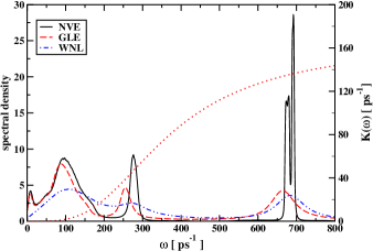
Figure 2: The spectra of SPC/Fw water computed from a microcanonical simulation (solid, black line), and simulations that employ the GLE - 12 fs colored noise parameter set (red, dashed line), and a white noise (blue, dot-dashed line) Langevin thermostat. The memory spectra that is obtained from the GLE dynamics is given by the red, dotted line. The strength of the white noise bath corresponds to the $\omega\rightarrow\infty$ limit of this profile ($\gamma=83.3$ ps^-1).

III Computational Details

The colored noise RESPA scheme introduced in the previous section was used to perform simulations of pure water and alanine dipeptide in explicit water. The water system consisted of 1000 molecules simulated in a 31.07 Å box. The alanine dipeptide was described by the OPLS-AA force field Jorgensen et al. (1996); Kaminski et al. (2001) in a 20 Å box containing 252 water molecules. The SPC/Fw potential Wu et al. (2006) was used to model the interactions between water molecules. All bonded terms (stretches, bends and torsions) were treated as flexible.

The forces were partitioned into three levels as in Eq. 36. The bonded terms were updated every 0.5 fs and the non bonded interactions below 9 Å were updated every 2 fs. The long range electrostatics, which dominate the computational cost of the simulation, were updated at the outer time step which was varied between 2 and 20 fs as discussed below. The electrostatics were partitioned into short and long range parts using the RESPA2 scheme. Stuart et al. (1996); Zhou et al. (2001) The function that switches between regions is a quintic spline which acts over a 4 Å region. Morrone et al. (2010) The cut off between the short and long range electrostatics was chosen so as to optimize the computational performance within our code. Larger cutoffs have been shown to produce better stability within the MTS formalism Han et al. (2007) so for maximum benefit the cutoffs used should be balanced with performance depending on the exact implementation.

Due to the cost of calculating the long range electrostatic interactions we wish to make the outer time step as large as possible while still obtaining correct sampling. We therefore performed simulations using time steps of 12 fs, 16 fs, and 20 fs. Resonance artifacts are extremely pronounced at these outer time steps so the simulation must be stabilized with either strong white noise damping or optimized colored noise thermostats. The baseline results for dynamic and equilibrium properties were obtained from a microcanonical and a white noise Langevin simulation, respectively and were performed using an outer time step of 2 fs. For the microcanonical results and each combination of thermostat and time step, water statistics were collected over twelve independent runs with initial velocities sampled from the Boltzmann distribution. For water a total of 12 ns of simulation time was performed, while for alanine dipeptide 400 ns was necessary to converge the properties reported.

IV Results and Discussion

For systems that exhibit large resonance artifacts, we now show that an appropriately designed colored noise thermostat is capable of yielding accurate sampling while simultaneously minimizing the thermostat’s impact on diffusional and orientational dynamics. In order to test this scheme, we perform simulations on flexible water and a fully flexible simulation of aqueous alanine dipeptide. The broad spectrum of frequencies in aqueous systems range from fast intramolecular stretches to slow diffusional modes (see Figure 2). The strong coupling between the modes makes this a challenging example to test our approach. Hence, for flexible water simulations the resonance barrier occurs at an outer time step of $\approx 3$ fs when the microcanonical r-RESPA algorithm is employed. Ma et al. (2003)

In this work, we design colored noise thermostats that are capable of stabilizing resonance artifacts for outer time steps of 12, 16, and 20 fs while ensuring that the error in the energies is within $0.5\%$ of the baseline results. The parameters for these thermostats are given in Table 1. In order to provide comparison as to the effectiveness of our scheme, we also perform simulations that use a white noise Langevin (WNL) thermostats to yield comparable accuracy. These runs utilize a friction of $14.2$ ps^-1, 40.0 ps^-1, and 100.0 ps^-1 in conjunction with outer times steps of 12 fs, 16 fs, and 20 fs, respectively.

Additionally, recent work has shown that when rigid constraints are placed on the fastest degrees of freedom, a weak Langevin coupling of $\gamma=1$ ps^-1 is required to stabilize the simulation at an outer time step of 12 fs. Han et al. (2007) We therefore perform simulations using a 2 fs outer time step with this friction. This facilitates a comparison of the dynamical perturbation arising from constrained dynamics using white noise stabilization with that caused by fully flexible dynamics using our colored noise scheme.

IV.1 Water

We first apply our scheme to pure flexible water. In Table 2 the average temperature and average bonded and non-bonded potential energies given for combinations of outer time step and method of resonance stabilization, either white noise Langevin (WNL) or generalized (colored noise) Langevin (GLE) thermostatting. The baseline result to which the static properties of all stabilized runs are compared utilizes an outer time step of $2$ fs and a WNL thermostat with a friction of $\gamma=1$ ps^-1. It can be seen that the GLE runs reproduce baseline results to within an error of $0.5\%$ for both the bonded and non-bonded components of the energy. The chosen white noise Langevin couplings exhibit comparable overall performance at each corresponding outer time step. Upon study of Table 2, it can be seen that the error is up to four times larger in the bonded energy as compared to the non-bonded energy for the GLE runs. In the case of the WNL stabilized simulations, it is up to ten times larger. This can be explained by the fact that resonance instabilities are most severe in the high frequency intramolecular modes. Therefore, as the error is not uniformly distributed across the system, it is of great utility to consider different components of the energy when assessing resonance stabilization. Although the error in the temperature is slightly elevated for runs with an outer time step of 20 fs, it is within $0.5\%$ for all other results. The errors in temperature tend to correlate with those in the potential energy. However, from the discussion above, the potential energy can be seen to be a more sensitive measure of sampling accuracy.

In Figure 3, the set of radial distributions of water of the GLE - 12 fs and GLE - 20 fs stabilized runs are shown to be in excellent agreement with the baseline calculations. The GLE - 16 fs results for clarity are not shown but are fully consistent with the other results. The inset shows that the peak corresponding to the oxygen hydrogen covalent bond is also well reproduced. This finding is significant since, as discussed above, the bonding energy tends to show a larger error than the overall energy. This reflects the fact that these components vary rapidly, thereby inducing a greater sensitivity to small deviations in position. Overall, the results of Figure 3 underline the fact that the free energy surface is accurately reproduced by the GLE resonance stabilized simulations.

Although both white and colored noise may be utilized to stabilize resonance artifacts, these two techniques significantly differ in the degree to which they disturb dynamical properties. In Table 3 we report the diffusion constant and the relaxation time of the first order molecular dipole orientational correlation function for the resonance stabilized simulations in comparison to the microcanonical baseline results. The colored noise stabilized dynamics with an outer time step of 12 fs differ by $4\%$ from the NVE results as compared to the difference of a factor of $2.5$ that is obtained from the WNL - 12 fs run. This finding is consistent with the selectivity of a colored noise thermostat which only couples weakly to the low frequency modes and therefore minimally perturbs dynamical quantities that largely depend upon these slower modes (see Fig. 2). It can be seen from Table 3 that the impact of the GLE - 12 fs profile on the dynamics is as good as and in some cases better than that of the weak white noise friction ($\gamma=1$ ps^-1) which is necessary to stabilize a simulation that employs constraints at a 12 fs outer time step. Han et al. (2007) Therefore the present method of targeted damping of fast modes compares very well to schemes where such modes are frozen.

The diffusion constant is extracted from the mean square displacement, which aside from its physical meaning, is also an indicator of the rate at which the simulation samples configuration space. Therefore, in addition to producing highly distorted dynamics, the strength of white noise coupling significantly slows down the sampling rate, largely counterbalancing any efficiency gained by utilizing a larger outer time step. Izaguirre et al. (2001) This drawback is alleviated by the use of the colored noise thermostat, although it can be clearly seen from Table 3 that the dynamical perturbation engendered by our scheme increases with outer time step as a “stronger” colored noise profile is necessary to stabilize the system. This arises naturally as a greater number of modes begin to resonate at larger outer time steps, thereby requiring strong coupling to the bath across lower frequency modes to damp out such artifacts. In this manner, increased disturbance of the dynamics is necessitated. The dynamics produced by the GLE - 16 fs and GLE - 20 fs runs differ from the baseline results by approximately $20\%$ and $35\%$, respectively. A comparison of the ratios of the GLE to the microcanonical results in Table 3 confirms that this degree of distortion can be reasonably estimated from Eq. (28). However, if only equilibrium properties are desired and the computational speed-up gained by increasing the outer time step outweighs the decrease in the sampling rate, these choices may still offer advantages.

thermostat	outer time step (fs)	T (K)	$V_{\text{nb}}/N$ (kcal/mol)	$V_{\text{b}}/N$ (kcal/mol)
WNL	2	$300.0$	$-3.872$	$0.5227$
GLE	12	$301.5$	$-3.869$	$0.5245$
GLE	16	$301.4$	$-3.869$	$0.5247$
GLE	20	$302.0$	$-3.872$	$0.5236$
WNL	12	$301.7$	$-3.875$	$0.5278$
WNL	16	$301.7$	$-3.874$	$0.5285$
WNL	20	$302.3$	$-3.875$	$0.5246$

Table 2: Average temperatures and bonded and non-bonded potential energies per atom of the flexible water system for different combinations of thermostat and outer time step. The figures are reported to a precision within the error of the calculation.

thermostat	outer time step (fs)	D ($\text{\AA}^{2}$/ps)	$\tau_{\text{dipole}}$ (ps)
NONE	2	$0.25$	$4.5$
WNL	2	$0.22$	$4.8$
GLE	12	$0.24$	$4.7$
GLE	16	0.20	5.6
GLE	20	0.16	6.7
WNL	12	0.095	8.0
WNL	16	0.044	14
WNL	20	0.019	26

Table 3: The dynamic quantities computed in the flexible water system. The diffusion constant and the first order molecular dipole relaxation time are given above. Figures are reported to statistical accuracy.

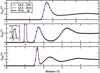
Figure 3: The atom-atom radial distribution functions of water computed from the baseline MTS white noise Langevin simulation with an an outer time step of 2 fs (black circles), is plotted against the colored noise thermostatted MTS prescription utilizing an outer time step of 12 fs (red solid line) and 20 fs (blue dashed line). The inset depicts the first peak of $g_{\text{OH}}(r)$ corresponding to the OH covalent bond.

IV.2 Alanine

Multiple time scale techniques are often employed to simulate biomolecular systems. In this section, we gauge the applicability of our scheme to a fully flexible simulation of alanine dipeptide in explicit water solvent. The use of this model system allows us to readily test the impact of the chosen colored noise profiles on conformational sampling and dynamics. The colored noise profiles utilized are the same as those presented in Section IV.1 and here we show their applicability to more general systems.

In Table 4 the energies of the alanine system for the chosen combinations of thermostats and outer time steps are presented. As in the case of pure water, the colored noise profiles reproduce the average bonded and non-bonded potential energies of the baseline (WNL - 2 fs) result to within $0.5\%$. The bonded energies include the stretches, bends, and torsions of alanine dipeptide in addition to the intramolecular interactions of water. As also noted in Section IV.1, the bonded energies, which contain high frequency modes and most strongly exhibit the resonance phenomena, possess a larger overall error than the non-bonded energies. This behavior underlines why our scheme of targeting fast motions for damping is successful. Additionally the total and alanine dipeptide temperature are reported, and can also be seen to be within $0.5\%$ of the baseline results.

The conformational space of alanine dipeptide is typically characterized as a function of the two dihedral angles $\psi$ and $\phi$. Hummer and Kevrekidis (2003); Chekmarev et al. (2004); Kwac et al. (2008) The Ramachandran plots of the baseline and GLE - 12 fs result are given in Figure 4. It can be seen that they are in excellent agreement. The resultant free energy exhibits a minimum in both the $\alpha$-helical and the extended $\text{P}_{\text{II}}$ region. These two regions are labeled in Figure 4.

The mean first passage time is estimated from the survival probability of the transition between the $\alpha_{R}$ and the $\text{P}_{\text{II}}$ regions. The survival probability, $S(t)$, for a state in the $\alpha_{R}$ region to cross to the $\text{P}_{\text{II}}$ region may be defined in terms of an average in conformation space over trajectories that reside in the $\alpha_{R}$ region at time $t=0$ and outside the $\text{P}_{\text{II}}$ region up to time, $t$ and is given by,

$$S_{\alpha_{R}\rightarrow\text{P}_{\text{II}}}(t) = \left<1-g_{\text{P}_{\text{II}}}(t)\right>_{h_{\alpha_{R}}(0)=1},$$ (40)

where $h_{\alpha_{R}}$ is unity inside the $\alpha_{R}$ region and zero outside, and $g_{\text{P}_{\text{II}}}(t)$ is defined to be unity if the particle has passed into region $\text{P}_{\text{II}}$ at any time between 0 and $t$ and is zero otherwise. The $\psi$ range of the $\alpha$-helical region is defined as $-40^{\circ}<\psi<10^{\circ}$ and the extended $\text{P}_{\text{II}}$ region as $110^{\circ}<\psi<180^{\circ}$. The $\phi$ range for both regions is set to be $-110^{\circ}<\phi<-60^{\circ}$.

The survival probabilities for the $\alpha_{R}\rightarrow\text{P}_{\text{II}}$ and $\text{P}_{\text{II}}\rightarrow\alpha_{R}$ transitions are plotted in Figure 5. The mean first passage times are presented in Table 5. The equilibrium constant of the $\alpha_{R}\rightleftharpoons\text{P}_{\text{II}}$ process is related to the ratio of the $\text{P}_{\text{II}}\rightarrow\alpha_{R}$ mean passage time to the $\alpha_{R}\rightarrow\text{P}_{\text{II}}$ value and is $\approx 1.8-1.9$ in all runs. Upon study of the mean first passage times, it can be seen that the colored noise thermostated result with an outer time step of 12 fs is perturbed by $\approx 10\%$ with respect to the microcanonical result, and is again comparable with the results of the system when weakly coupled to a white noise bath ($\gamma=1$ ps^-1). The colored noise thermostat causes a slightly larger perturbation on the mean passage time when compared to that exhibited in the diffusion of water (see Sec. IV.1). This likely arises from the dependence of this property on torsional motions that lie in a higher frequency range than diffusive modes, and are therefore more strongly coupled to the bath. The large white noise friction that is necessary to damp out resonance instabilities at an outer time step of 12 fs again increases passage times by a factor of $\approx 2.5$. The impact of large WNL couplings on the conformational dynamics has been noted in previous work. Derreumaux and Schlick (1995) As in the case of pure water, the degree of perturbation induced by the GLE thermostat increases as a greater degree of energy stabilization is necessary at larger outer time steps. The similarity of the results obtained in this case and pure water underlines the fact the thermostatting scheme presented in this work is transferable between flexible water and typical solvated biomolecules.

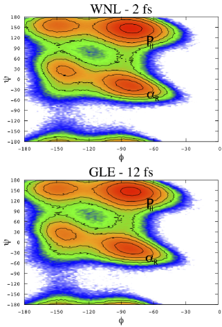
Figure 4: The free energy as a function of dihedral angles $\phi$ and $\psi$. The baseline WNL - 2fs (top panel) and GLE - 12fs (bottom panel) results are shown. The free energy in conformation space decreases as the color varies from white to red. Isolines represent increments of 0.5 kcal/mol. The $\alpha_{R}$ and $\text{P}_{\text{II}}$ regions are labeled in each panel.

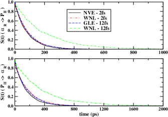
Figure 5: The survival probabilities for selected runs of the alanine dipeptide system are shown for the transition from the $\alpha_{R}$ to $\text{P}_{\text{II}}$ region (top panel) and for the reverse process (bottom panel). Results are given for the baseline microcanonical (solid black curve) and white noise Langevin (red dot-dashed curve) runs as well as the simulations that are resonance stabilized with an outer time step of 12 fs utilizing colored (blue dashed curve) and white (green dot-dashed curve) noise.

thermostat	outer time step (fs)	T(K)	T${}_{\text{ALA}}$ (K)	$V_{\text{nb}}/N$ (kcal/mol)	$V_{\text{b}}/N$ (kcal/mol)
WNL	2	$300.0$	$299.7$	$-3.828$	$0.5297$
GLE	12	$301.0$	$300.1$	$-3.825$	$0.5312$
GLE	16	$301.1$	$299.8$	$-3.823$	$0.5314$
GLE	20	$301.7$	$299.8$	$-3.826$	$0.5304$
WNL	12	301.3	300.0	$-3.829$	$0.5338$
WNL	16	301.4	299.8	$-3.828$	$0.5344$
WNL	20	$302.0$	$300.0$	$-3.828$	$0.5315$

Table 4: The total and alanine dipeptide temperatures, as well as the bonded and non-bonded energy per atom are given for each combination of outer time step and thermostatting scheme utilized for alanine dipeptide in explicit solvent. The figures are reported to statistical accuracy.

thermostat	outer time step (fs)	$\bar{\tau}(\alpha_{R}\rightarrow\text{P}_{\text{II}})$ (ps)	$\bar{\tau}(\text{P}_{\text{II}}\rightarrow\alpha_{R})$ (ps)
NONE	2	79	142
WNL	2	85	163
GLE	12	87	156
GLE	16	105	193
GLE	20	121	234
WNL	12	190	340
WNL	16	435	790

Table 5: Table of mean first passage times, $\bar{\tau}$, from the $\alpha_{R}$ to $\text{P}_{\text{II}}$ and $\text{P}_{\text{II}}$ to $\alpha_{R}$ regions are presented for various combinations of outer time steps and thermostatting schemes. The average error for runs where the dynamics are not strongly overdamped is $\approx 3$ ps. Results are not given for the WNL - 20 fs run due to the fact that too few transitions occurred in the course of the simulation to generate a reliable estimate of $\bar{\tau}$.

V Conclusions

In this paper, we have shown that by coupling a standard multiple time scale scheme to a colored noise bath large outer time steps can be employed while obtaining accurate sampling and minimally perturbing the dynamics. The scheme was illustrated with applications to flexible water and a fully flexible simulation of aqueous alanine dipeptide. Our results suggest that, when combined with our scheme, a 12 fs outer time step seems a good compromise between size of outer time step and minimizing the impact on the dynamics. With this outer time step the damping needed to obtain potential energies within $0.5\%$ of the benchmark values decreased diffusion by only $4\%$. In contrast, stabilization of the simulation at this outer time step using white noise decreases the diffusion constant by over 2.5 times. Even more promising, the dynamical perturbation due to our colored noise scheme compared favorably with the weak white noise damping ($\gamma=1$ ps^-1) required to stabilize a multiple time scale simulation in which all bonds to hydrogen are constrained. Han et al. (2007) This suggests that, in conjunction with multiple time scale algorithms, this method may be utilized in lieu of constraints.

In our serial code using a 12 fs outer time step yielded a computational speed-up of 4.3 times compared to our baseline MTS calculations using a 2 fs outer time step and a 17 times speed up compared to flexible simulations without a multiple time scale scheme that employ a 0.5 fs time step. Even further increases may be achieved when the computational architecture or parallelization scheme makes long range electrostatics comparatively costly to evaluate. Bowers et al. (2006) It is therefore clear that this scheme provides an efficient approach to perform equilibration or configurational sampling. Although our approach perturbs the dynamics we note that the alanine dipeptide molecule used in our benchmark simulation was specifically chosen to allow us to view many transitions and hence converge the dynamical properties within small bounds. In typical, large-scale biological system where long time-scale processes are of interest this would not be the case and hence the small change in the dynamics due to this method will likely be dwarfed by the statistical errors. In this case the ability to generate longer trajectories using this approach facilitates a decrease in the statistical errors bars.

The similarities in the spectra of many aqueous and biological systems suggest that our noise profiles should provide good out-of-the box performance for other fully flexible systems. However, the flexibility of the colored noise approach affords such a large degree of versatility that further tuning may yield improved results. Our matrices may also provide a basis for other applications where energy must be rapidly dissipated to ensure accurate sampling such as in the case of fast-deposition metadynamics. Ceriotti (2010) The methods outlined in Sec. II and Appendix A provide a starting point for such developments.

Appendix A Further applications of simple drift matrices

It is often convenient to consider drift matrices whose elements are transparently related to the time dependence of the memory kernel (i.e. the eigenvalues of submatrix $\bm{\mathrm{\Gamma}}_{ss}$). This facilitates the use of readily tunable colored noise profiles that are based on a small set of parameters. In addition to the form presented in this work (Eq. (25)), two other of such matrices have appeared in the literature. The drift matrix for a simple exponential noise is given by Ceriotti et al. (2009a)

$$\bm{\mathrm{\Gamma}}_{\text{A}} = \left(\begin{array}[]{cc}0&\sqrt{\gamma_{0}a}\\ -\sqrt{\gamma_{0}a}&a\end{array}\right)$$ (43)

where the memory function and spectra are:

$$K_{\text{A}}(t) = \gamma_{0}ae^{-|t|a}$$ (44)

$$\hat{K}_{\text{A}}(\omega) = 2\gamma_{0}a\frac{a}{a^{2}+\omega^{2}}.$$ (45)

Whereas the following drift matrix, Ceriotti and Parrinello (2010)

$$\bm{\mathrm{\Gamma}}_{\text{B}} = \left(\begin{array}[]{ccc}0&\sqrt{\frac{\gamma_{0}(a^{2}+b^{2})}{2a}}&\sqrt{\frac{\gamma_{0}(a^{2}+b^{2})}{2a}}\\ -\sqrt{\frac{\gamma_{0}(a^{2}+b^{2})}{2a}}&a&b\\ -\sqrt{\frac{\gamma_{0}(a^{2}+b^{2})}{2a}}&-b&a\end{array}\right),$$ (49)

corresponds to a term of damped oscillatory noise whose spectra is centered at $\pm b$:

$$K_{\text{B}}(t) = \gamma_{0}\frac{a^{2}+b^{2}}{a}e^{-|t|a}\cos(bt)$$ (50)

$$\hat{K}_{\text{B}}(\omega) = \gamma_{0}\frac{a^{2}+b^{2}}{a}\left(\frac{a}{a^{2}+\left(\omega-b\right)^{2}}+\frac{a}{a^{2}+\left(\omega+b\right)^{2}}\right).$$ (51)

In the above equations, the parameter, $a$, corresponds to the real part and $b$ to the magnitude of the imaginary part of the eigenvalue(s) of submatrix, $\bm{\mathrm{\Gamma}}_{ss}$. As in Section II, the parameter $\gamma_{0}$ is proportional to the value of the memory spectra at $\omega=0$, such that $\hat{K}(0)=2\gamma_{0}$.

Drift matrices that correspond to stable dynamics may be combined such that the resultant memory function is a weighted sum of the corresponding memory functions of each component. Ceriotti and Parrinello (2010) For example, the drift matrix that corresponds to the sum of the noise profiles of whose drift matrices are given by ${}^{1}\bm{\mathrm{\Gamma}}$ and ${}^{2}\bm{\mathrm{\Gamma}}$ is given by,

$${}^{(1+2)}\bm{\mathrm{\Gamma}} = \left(\begin{array}[]{ccc}(^{1}\gamma_{pp}+^{2}\gamma_{pp})&{}^{1}\bm{\gamma}_{ps}^{T}&{}^{2}\bm{\gamma}_{ps}^{T}\\ ^{1}\bm{\gamma}_{sp}&{}^{1}\bm{\mathrm{\Gamma}}_{ss}&\bm{\mathrm{0}}\\ ^{2}\bm{\gamma}_{sp}&\bm{\mathrm{0}}&{}^{2}\bm{\mathrm{\Gamma}}_{ss}\end{array}\right)$$ (55)

where components are expressed in the notation of Eq. (18) . In this way, forms such as those presented here may be utilized as “building blocks” for more flexible colored noise profiles.

Making use of this machinery, it is possible to design a form that couples strongly to certain modes and weakly to others. Eq. (55) may be applied to add together noise profiles of the damped oscillatory (Eq. (51)) or the “canceling” (Eq. (27)) type. It must be noted that this formalism has drawbacks when compared to the profiles utilized in the main text. Namely, the dimensionality of the resultant drift matrix grows with the number of targeted modes and that the greater sensitivity to the details of the spectra implies less robust performance across different systems. However, this sensitivity also facilitates fine control of the colored noise profile for very specific applications.

Appendix B Dynamical properties of a GLE dynamics

In order to estimate the perturbation on the dynamical properties of a system caused by coupling to a colored noise thermostat one can study the behavior of a one-dimensional harmonic model. In this limit, microcanonical dynamical results in a $\delta$-function power spectrum peaked at the oscillator’s characteristic frequency $\omega_{0}$. The presence of the noise will modify the line shape of the peak, shifting its center and broadening it. A measure of these two effects can be used to estimate the magnitude of the disturbance.

To achieve this, one must consider the matrices $\bm{\Gamma}_{qp}\left(\omega_{0}\right)$ and $\mathbf{B}_{qp}\left(\omega_{0}\right)$ which describe the dynamics in the full $\mathbf{x}=\left(q,p,\mathbf{s}\right)$ space. Ceriotti et al. (2010a) One can then find the stationary covariance matrix $\mathbf{C}_{qp}$ by solving $\bm{\Gamma}_{qp}\mathbf{C}_{qp}+\mathbf{C}_{qp}\bm{\Gamma}_{qp}^{T}=\mathbf{B}_{qp}\mathbf{B}_{qp}^{T}$ and compute the first order correlation matrix $\left\langle\mathbf{x}^{T}\left(t\right)\mathbf{x}\left(0\right)\right\rangle$ and its Fourier transform,

$$\mathcal{C}_{ij}\left(\omega\right)=\left[\frac{\bm{\Gamma}_{qp}}{\bm{\Gamma}_{qp}^{2}+\omega^{2}}\mathbf{C}_{qp}\right]_{ij}\left[\left(\mathbf{C}_{qp}\right)_{ii}\left(\mathbf{C}_{qp}\right)_{jj}\right]^{-1/2}.$$ (56)

The position and value at the maximum of the $\mathcal{C}_{pp}\left(\omega\right)$ term can then be used to characterize the deformed peak.

When $\bm{\Gamma}_{qp}$ is built out of the $3\times 3$ canceling noise matrix in Eq. (25) and we set $\gamma_{0}=0$ so as to consider the case of small disturbance on the low-frequency modes we obtain,

$$\bm{\Gamma}_{qp}=\left(\begin{array}[]{cccc}0&-1&0&0\\ \omega_{0}^{2}&\gamma&\sqrt[4]{3}\sqrt{\gamma\tilde{\omega}}&\sqrt{\gamma\tilde{\omega}}/\sqrt[4]{3}\\ 0&\sqrt[4]{3}\sqrt{\gamma\tilde{\omega}}&\sqrt{3}\tilde{\omega}&\tilde{\omega}\\ 0&-\sqrt{\gamma\tilde{\omega}}/\sqrt[4]{3}&-\tilde{\omega}&0\end{array}\right).$$ (61)

Solving for $\mathcal{C}_{pp}\left(\omega\right)$ we obtain

$$\mathcal{C}_{pp}\left(\omega\right) = \frac{3\gamma\omega^{6}}{\gamma^{2}\omega^{4}\left(3\omega^{2}+\tilde{\omega}^{2}\right)+2\sqrt{3}\gamma\tilde{\omega}\omega^{2}\left(\omega^{2}-\omega_{0}^{2}\right)\left(2\omega^{2}+\tilde{\omega}^{2}\right)+3\left(\omega^{2}-\omega_{0}^{2}\right)^{2}\left(\omega^{4}+\tilde{\omega}^{2}\omega^{2}+\tilde{\omega}^{4}\right)}$$ (62)

We then take $\tilde{\omega}$ to be much larger than all other frequencies entering our problem, and write them as a ratio with respect to $\tilde{\omega}$, i.e. $\omega_{0}\leftarrow\omega_{0}/\tilde{\omega}$, $\gamma\leftarrow\gamma/\tilde{\omega}$, $\omega\leftarrow\omega/\tilde{\omega}$. One then finds the relevant extremal point, $\omega_{P}$, and an estimate of the peak width as $\Delta_{P}=1/\left[\pi\mathcal{C}_{pp}\left(\omega_{P}\right)\right]$. This leads to expressions which can then be expanded in powers of $\omega_{0}$, eventually yielding

$$\omega_{P}=\frac{\omega_{0}}{\sqrt{1+\frac{\gamma/\tilde{\omega}}{\sqrt{3}}}}+\mathcal{O}\left(\left(\omega_{0}/\tilde{\omega}\right)^{2}\right)$$ (63)

and

$$\Delta_{P}=\frac{\gamma\left(\omega_{0}/\tilde{\omega}\right)^{4}}{\pi\left(1+\frac{\gamma/\tilde{\omega}}{\sqrt{3}}\right)^{2}}+\mathcal{O}\left(\left(\omega_{0}/\tilde{\omega}\right)^{6}\right).$$ (64)

References

- Streett et al. (1978) W. Streett, D. J. Tildesley, and G. Saville, Mol. Phys. 35, 639 (1978).
- Tuckerman et al. (1990) M. E. Tuckerman, G. J. Martyna, and B. J. Berne, J. Chem. Phys. 93, 1287 (1990).
- Grubmuller et al. (1991) H. Grubmuller, H. Heller, A. Windemuth, and K. Schulten, Molecular Simulation 6, 121 (1991).
- Tuckerman et al. (1992) M. Tuckerman, B. J. Berne, and G. J. Martyna, J. Chem. Phys. 97, 1990 (1992).
- Biesaideki and Skeel (1993) J. J. Biesaideki and R. D. Skeel, J. Comput. Phys. 109, 318 (1993).
- Ma et al. (2003) Q. Ma, J. A. Izaguirre, and R. D. Skeel, Siam J. Sci. Comput. 24, 1951 (2003).
- Izaguirre et al. (1999) J. A. Izaguirre, S. Reich, and R. D. Skeel, J. Chem. Phys. 110, 9853 (1999).
- Zhou et al. (2001) R. Zhou, E. Harder, H. Xu, and B. J. Berne, J. Chem. Phys. 115, 2348 (2001).
- Han et al. (2007) G. Han, Y. Deng, J. Glimm, and G. J. Martyna, Comput. Phys. Comm. 176, 271 (2007).
- Izaguirre et al. (2001) J. A. Izaguirre, D. P. Catarello, J. M. Wozniak, and R. D. Skeel, J. Chem. Phys. 114, 2090 (2001).
- Ma and Izaguirre (2003) Q. Ma and J. A. Izaguirre, Multiscale Model. Simul. 2, 1 (2003).
- Barth and Schlick (1998) E. Barth and T. Schlick, J. Chem. Phys. 109, 1617 (1998).
- Qian and Schlick (2002) X. Qian and T. Schlick, J. Chem. Phys. 116, 5971 (2002).
- Minary et al. (2004) P. Minary, M. E. Tuckerman, and G. J. Martyna, Phys. Rev. Lett. 93, 150201 (2004).
- Sweet et al. (2008) C. R. Sweet, P. Petrone, V. S. Pande, and J. A. Izaguirre, J. Chem. Phys. 128, 145101 (2008).
- Ceriotti et al. (2009a) M. Ceriotti, G. Bussi, and M. Parrinello, Phys. Rev. Lett. 102, 020601 (2009a).
- Ceriotti et al. (2009b) M. Ceriotti, G. Bussi, and M. Parrinello, Phys. Rev. Lett. 103, 030603 (2009b).
- Ceriotti et al. (2010a) M. Ceriotti, G. Bussi, and M. Parrinello, J. Chem. Theory Comput. 6, 1170 (2010a).
- Ceriotti and Parrinello (2010) M. Ceriotti and M. Parrinello, Procedia Computer Science 1, 1601 (2010).
- Ceriotti et al. (2010b) M. Ceriotti, M. Parrinello, T. E. Markland, and D. E. Manolopoulos, J. Chem. Phys. 133, 124104 (2010b).
- Berne and Pecora (2000) B. J. Berne and R. Pecora, Dynamic Light Scattering (Dover, New York, 2000).
- Zwanzig (2001) R. Zwanzig, Nonequilibrium statistical mechanics (Oxford University Press, 2001).
- Gardiner (2009) C. Gardiner, Stochastic Methods: A Handbook for the Natural and Social Sciences (Springer-Verlag, Berlin, 2009), 4th ed.
- Ferrario and Grigolini (1979) M. Ferrario and P. Grigolini, J. Math. Phys. 20, 2567 (1979).
- Marchesoni and Grigolini (1983) F. Marchesoni and P. Grigolini, J. Chem. Phys. 78, 6287 (1983).
- Berne (1971) B. J. Berne, Physical Chemistry (Academic Press, New York, 1971), vol. VIIIB, chap. 9, p. 539.
- Tuckerman and Berne (1993) M. E. Tuckerman and B. J. Berne, J. Chem. Phys. 98, 7301 (1993).
- Wu et al. (2006) Y. J. Wu, H. L. Tepper, and G. A. Voth, J. Chem. Phys. 124, 024503 (2006).
- Bussi and Parrinello (2007) G. Bussi and M. Parrinello, Phys. Rev. E 75, 056707 (2007).
- Martyna et al. (1992) G. J. Martyna, M. L. Klein, and M. Tuckerman, J. Chem. Phys. 97, 2635 (1992).
- Martyna et al. (1996) G. J. Martyna, M. E. Tuckerman, D. J. Tobias, and M. L. Klein, Mol. Phys. 87, 1117 (1996).
- Jorgensen et al. (1996) W. L. Jorgensen, D. S. Maxwell, and J. Tirado-Rives, J. Am. Chem. Soc. 118, 11225 (1996).
- Kaminski et al. (2001) G. Kaminski, R. A. Friesner, J. Tirado-Rives, and W. L. Jorgensen, J. Phys. Chem. B 105, 6474 (2001).
- Stuart et al. (1996) S. J. Stuart, R. Zhou, and B. J. Berne, J. Chem. Phys. 105, 1426 (1996).
- Morrone et al. (2010) J. A. Morrone, R. Zhou, and B. J. Berne, J. Chem. Theory Comput. 6, 1798 (2010).
- Hummer and Kevrekidis (2003) G. Hummer and I. G. Kevrekidis, J. Chem. Phys. 118, 10762 (2003).
- Chekmarev et al. (2004) D. S. Chekmarev, T. Ishida, and R. M. Levy, J. Phys. Chem. B 108, 19487 (2004).
- Kwac et al. (2008) K. Kwac, K. Lee, J. Han, K. Oh, and M. Cho, J. Chem. Phys. 128, 105106 (2008).
- Derreumaux and Schlick (1995) P. Derreumaux and T. Schlick, Proteins: Structure, Function, and Genetics 21, 282 (1995).
- Bowers et al. (2006) K. Bowers, E. Chow, H. Xu, R. Dror, M. Eastwood, B. Kolossvary, M. Moraes, F. Sacerdoti, J. Salmon, Y. Shan, et al., in Proceedings of the ACM/IEEE Conference on Supercomputing (SC06) (Tampa, Florida, 2006).
- Ceriotti (2010) M. Ceriotti, Ph.D. thesis n. 19083, ETH Zürich (2010).