Statistical and knowledge supported visualization of multivariate data.
Abstract In the present work we have selected a collection of statistical and mathematical tools useful for the exploration of multivariate data and we present them in a form that is meant to be particularly accessible to a classically trained mathematician. We give self contained and streamlined introductions to principal component analysis, multidimensional scaling and statistical hypothesis testing. Within the presented mathematical framework we then propose a general exploratory methodology for the investigation of real world high dimensional datasets that builds on statistical and knowledge supported visualizations. We exemplify the proposed methodology by applying it to several different genomewide DNA-microarray datasets. The exploratory methodology should be seen as an embryo that can be expanded and developed in many directions. As an example we point out some recent promising advances in the theory for random matrices that, if further developed, potentially could provide practically useful and theoretically well founded estimations of information content in dimension reducing visualizations. We hope that the present work can serve as an introduction to, and help to stimulate more research within, the interesting and rapidly expanding field of data exploration.
1 Introduction.
In the scientific exploration of some real world phenomena a lack of detailed knowledge about governing first principles makes it hard to construct well-founded mathematical models for describing and understanding observations. In order to gain some preliminary understanding of involved mechanisms and to be able to make some reasonable predictions we then often have to recur to purely statistical models. Sometimes though, a stand alone and very general statistical approach fails to exploit the full exploratory potential for a given dataset. In particular a general statistical model a priori often does not incorporate all the accumulated field-specific expert knowledge that might exist concerning a dataset under consideration. In the present work we argue for the use of a set of statistical and knowledge supported visualizations as the backbone of the exploration of high dimensional multivariate datasets that are otherwise hard to model and analyze. The exploratory methodology we propose is generic but we exemplify it by applying it to several different datasets coming from the field of molecular biology. Our choice of example application field is in principle anyhow only meant to be reflected in the list of references where we have consciously striven to give references that should be particularly useful and relevant for researchers interested in bioinformatics. The generic case we have in mind is that we are given a set of observations of several different variables that presumably have some interrelations that we want to uncover. There exist many rich real world sources giving rise to interesting examples of such datasets within the fields of e.g. finance, astronomy, meteorology or life science and the reader should without difficulty be able to pick a favorite example to bear in mind.
We will use separate but synchronized Principle Component Analysis (PCA) plots of both variables and samples to visualize datasets. The use of separate but synchronized PCA-biplots that we argue for is not standard and we claim that it is particularly advantageous, compared to using traditional PCA-biplots, when the datasets under investigation are high dimensionsional. A traditional PCA-biplot depicts both the variables and the samples in the same plot and if the dataset under consideration is high dimensional such a joint variable/sample plot can easily become overloaded and hard to interpret. In the present work we give a presentation of the linear algebra of PCA accentuating the natural inherent duality of the underlying singular value decomposition. In addition we point out how the basic algorithms easily can be adapted to produce nonlinear versions of PCA, so called multidimensional scaling, and we illustrate how these different versions of PCA can reveal relevant structure in high dimensional and complex real world datasets. Whether an observed structure is relevant or not will be judged by knowledge supported and statistical evaluations.
Many present day datasets, coming from the application fields mentioned above, share the statistically challenging peculiarity that the number of measured variables () can be very large (), while at the same time the number of observations () sometimes can be considerably smaller (). In fact all our example datasets will share this so called ”large small ” characteristic and our exploratory scheme, in particular the statistical evaluation, is well adapted to cover also this situation. In traditional statistics one usually is presented with the reverse situation, i.e. ”large small ”, and if one tries to apply traditional statistical methods to ”large small ” datasets one sometimes runs into difficulties. To begin with, in the applications we have in mind here, the underlying probability distributions are often unknown and then, if the number of observations is relatively small, they are consequently hard to estimate. This makes robustness of employed statistical methods a key issue. Even in cases when we assume that we know the underlying probability distributions or when we use very robust statistical methods the ”large small ” case presents difficulties. One focus of statistical research during the last few decades has in fact been driven by these ”large small ” datasets and the possibility for fast implementations of statistical and mathematical algorithms. An important example of these new trends in statistics is multiple hypothesis testing on a huge number of variables. High dimensional multiple hypothesis testing has stimulated the creation of new statistical tools such as the replacement of the standard concept of p-value in hypothesis testing with the corresponding q-value connected with the notion of false discovery rate, see [12], [13], [48], [49] for the seminal ideas. As a remark we point out that multivariate statistical analogues of classical univariate statistical tests sometimes can perform better in multiple hypothesis testing, but then a relatively small number of samples normally makes it necessary to first reduce the dimensionality of the data, for instance by using PCA, in order to be able to apply the multivariate tests, see e.g. [14], [33], [32] for ideas in this direction. In the present work we give an overview and an introduction to the above mentioned statistical notions.
The present work is in general meant to be one introduction to, and help to stimulate more research within, the field of data exploration. We also hope to convince the reader that statistical and knowledge supported visualization already is a versatile and powerful tool for the exploration of high dimensional real world datasets. Finally, ”Knowledge supported” should here be interpreted as ”any use of some extra information concerning a given dataset that the researcher might possess, have access to or gain during the exploration” when analyzing the visualization. We illustrate this knowledge supported approach by using knowledge based annotations coming with our example datasets. We also briefly comment on how to use information collected from available databases to evaluate or preselect groups of significant variables, see e.g. [11],[16], [31],[42] for some more far reaching suggestions in this direction.
2 Singular value decomposition and Principal component analysis.
Singular value decomposition (SVD) was discovered independently by several mathematicians towards the end of the 19’th century. See [47] for an account of the early history of SVD. Principal component analysis (PCA) for data analysis was then introduced by Pearson [25] in 1901 and independently later developed by Hotelling [24]. The central idea in classical PCA is to use an SVD on the column averaged sample matrix to reduce the dimensionality in the data set while retaining as much variance as possible. PCA is also closely related to the Karhunen-Loève expansion (KLE) of a stochastic process [29], [34]. The KLE of a given centered stochastic process is an orthonormal -expansion of the process with coefficients that are uncorrelated random variables. PCA corresponds to the empirical or sample version of the KLE, i.e. when the expansion is inferred from samples. Noteworthy here is the Karhunen–Loève theorem stating that if the underlying process is Gaussian, then the coefficients in the KLE will be independent and normally distributed. This is e.g. the basis for showing results concerning the optimality of KLE for filtering out Gaussian white noise.
PCA was proposed as a method to analyze genomewide expression data by Alter et al. [1] and has since then become a standard tool in the field. Supervised PCA was suggested by Bair et.al. as a regression and prediction method for genomewide data [8], [9], [17]. Supervised PCA is similar to normal PCA, the only difference being that the researcher preconditions the data by using some kind of external information. This external information can come from e.g. a regression analysis with respect to some response variable or from some knowledge based considerations. We will here give an introduction to SVD and PCA that focus on visualization and the notion of using separate but synchronized biplots, i.e. plots of both samples and variables. Biplots displaying samples and variables in the same usually twodimensional diagram have been used frequently in many different types of applications, see e.g. [20], [21], [22] and [15], but the use of separate but synchronized biplots that we present is not standard. We finally describe the method of multidimensional scaling which builds on standard PCA, but we start by describing SVD for linear operators between finite dimensional euclidean spaces with a special focus on duality.
2.1 Dual singular value decomposition
Singular value decomposition is a decomposition of a linear mapping between euclidean spaces. We will discuss the finite dimensional case and we consider a given linear mapping .
Let be the canonical basis in and let be the canonical basis in . We regard and as euclidean spaces equipped with their respective canonical scalar products, and , in which the canonical bases are orthonormal.
Let denote the adjoint operator of defined by
| (2.1) |
Observe that in applications , , normally represent the arrays of observed variable values for the different samples and that , , then represent the observed values of the variables. In our example data sets, the unique matrix representing in the canonical bases, i.e.
contains measurements for all variables in all samples. The transposed matrix contains the same information and represents the linear mapping in the canonical bases.
The goal of a dual SVD is to find orthonormal bases in and such that the matrices representing the linear operators and have particularly simple forms.
We start by noting that directly from (2.1) we get the following direct sum decompositions into orthogonal subspaces
(where denotes the kernel of and denotes the image of ) and
We will now make a further dual decomposition of and .
Let denote the rank of , i.e. . The rank of the positive and selfadjoint operator is then also equal to , and by the spectral theorem there exist values and corresponding orthonormal vectors , with , such that
| (2.2) |
If , i.e. , then zero is also an eigenvalue for with multiplicity .
Using the orthonormal set of eigenvectors for spanning , we define a corresponding set of dual vectors in by
| (2.3) |
From (2.2) it follows that
| (2.4) |
and that
| (2.5) |
The set of vectors defined by (2.3) spans and is an orthonormal set of eigenvectors for the selfadjoint operator . We thus have a completely dual setup and canonical decompositions of both and into direct sums of subspaces spanned by eigenvectors corresponding to the distinct eigenvalues. We make the following definition.
Definition 2.1
A dual singular value decomposition system for an operator pair (, ) is a system consisting of numbers and two sets of orthonormal vectors, and with , satisfying (2.2)–(2.5) above.
The positive values are called the singular values of (, ). We will call the vectors principal components for and the vectors principal components for .
Given a dual SVD system we now complement the principal components for , , to an orthonormal basis in and the principal components for , , to an orthonormal basis in .
In these bases we have that
| (2.6) |
This means that in these ON-bases is represented by the diagonal matrix
| (2.7) |
where is the diagonal matrix having the singular values of (, ) in descending order on the diagonal. The adjoint operator is represented in the same bases by the transposed matrix, i.e. a diagonal matrix.
We translate this to operations on the corresponding matrices as follows. Let denote the matrix having the coordinates, in the canonical basis in , for as columns, and let denote the matrix having the coordinates, in the canonical basis in , for as columns. Then (2.6) is equivalent to
This is called a dual singular value decomposition for the pair of matrices (, ).
Notice that the singular values and the corresponding separate eigenspaces for as described above are canonical, but that the set (and thus also the connected set ) is not canonically defined by . This set is only canonically defined up to actions of the appropriate orthogonal groups on the separate eigenspaces.
2.2 Dual principal component analysis
We will now discuss how to use a dual SVD system to obtain optimal approximations of a given operator by operators of lower rank. If our goal is to visualize the data, then it is natural to measure the approximation error using a unitarily invariant norm, i.e. a norm that is invariant with respect to unitary transformations on the variables or on the samples, i.e.
| (2.8) |
Using an SVD, directly from (2.8) we conclude that such a norm is necessarily a symmetric function of the singular values of the operator. We will present results for the –norm of the singular values, but the results concerning optimal approximations are actually valid with respect to any unitarily invariant norm, see e.g. [35] and [40] for information in this direction. We omit proofs, but all the results in this section are proved using SVDs for the involved operators.
The Frobenius (or Hilbert-Schmidt) norm for an operator of rank is defined by
where , are the singular values of (, ).
Now let denote the set of real matrices. We then define the set of orthogonal projections in of rank as
One important thing about orthogonal projections is that they never increase the Frobenius norm, i.e.
Lemma 2.1
Let be a given linear operator. Then
and
Using this Lemma one can prove the following approximation theorems.
Theorem 2.1
Let be a given linear operator. Then
| (2.9) |
and equality is attained in (2.1) by projecting onto the first principal components for and .
Theorem 2.2
Let be a given linear operator. Then
| (2.10) |
and equality is attained in (2.2) by projecting onto the first principal components for and .
We loosely state these results as follows.
Projection dictum
Projecting onto a set of first principal components maximizes average projected vector length and also minimizes average projection error.
We will briefly discuss interpretation for applications. In fact in applications the representation of our linear mapping normally has a specific interpretation in the original canonical bases. Assume that , represent samples and that , represents variables. To begin with, if the samples are centered, i.e.
then corresponds to the statistical variance of the sample set. The basic projection dictum can thus be restated for sample-centered data as follows.
Projection dictum for sample-centered data
Projecting onto a set of first principal components maximizes the variance in the set of projected data points and also minimizes average projection error.
In applications we are also interested in keeping track of the value
| (2.11) |
It represents the ’th variable’s value in the ’th sample.
Computing in a dual SVD system for (, ) in (2.11) we get
| (2.12) |
Now using (2.3) and (2.4) we conclude that
Finally this implies the fundamental biplot formula
| (2.13) |
We now introduce the following scalar product in
Equation (2.13) thus means that if we express the sample vectors in the basis for and the variable vectors in the basis for , then we get the value of simply by taking the -scalar product in between the coordinate sequence for the k’th sample and the coordinate sequence for the j’th variable.
This means that if we work in a synchronized way in with the coordinates for the samples (with respect to the basis ) and with the coordinates for the variables (with respect to the basis ) then the relative positions of the coordinate sequence for a variable and the coordinate sequence for a sample in have a very precise meaning given by (2.13).
Now let be a subset of indices and let denote the number of elements in . Then let be the orthogonal projection onto the subspace spanned by the principal components for whose indices belong to . In the same way let be the orthogonal projection onto the subspace spanned by the principal components for whose indices belong to .
If , represent samples, then , , represent -approximative samples, and correspondingly if , , represent variables then , , represent -approximative variables.
We will interpret the matrix element
| (2.14) |
as representing the ’th -approximative variable’s value in the ’th -approximative sample.
By the biplot formula (2.13) for the operator we actually have
| (2.15) |
If we can visualize our approximative samples and approximative variables working in a synchronized way in with the coordinates for the approximative samples and with the coordinates for the approximative variables. The relative positions of the coordinate sequence for an approximative variable and the coordinate sequence for an approximative sample in then have the very precise meaning given by (2.15).
Naturally the information content of a biplot visualization depends in a crucial way on the approximation error we make. The following result gives the basic error estimates.
Theorem 2.3
With notations as above we have the following projection error estimates
| (2.16) | |||
| (2.17) |
We will use the following statistics for measuring projection content:
Definition 2.2
With notations as above, the -projection content connected with the subset is by definition
We note that, in the case when we have sample centered data, is precisely the quotient between the amount of variance that we have ”captured” in our projection and the total variance. In particular if then we have captured all the variance. Theorem 2.3 shows that we would like to have good control of the distributions of eigenvalues for general covariance matrices. We will address this issue for random matrices below, but we already here point out that we will estimate projection information content, or the signal to noise ratio, in a projection of real world data by comparing the observed -projection content and the -projection contents for corresponding randomized data.
2.3 Nonlinear PCA and multidimensional scaling
We begin our presentation of multidimensional scaling by looking at the reconstruction problem, i.e. how to reconstruct a dataset given only a proposed covariance or distance matrix. In the case of a covariance matrix, the basic idea is to try to factor a corresponding sample centered SVD or slightly rephrased by taking the square root of the covariance matrix.
Once we have established a reconstruction scheme we note that we can apply it to any proposed ”covariance” or ”distance” matrix, as long as they have the correct structure, even if they are artificial and a priori are not constructed using euclidean transformations on an existing data matrix. This opens up the possibility for using ”any type” of similarity measures between samples or variables to construct artificial covariance or distance matrices.
We consider a matrix where the columns consist of values of measurements for samples of variables. We will throughout this section assume that . We introduce the vector
and we recall that the covariance matrix of the data matrix is given as
We will also need the (squared) distance matrix defined by
We will now consider the problem of reconstructing a data matrix given only the corresponding covariance matrix or the corresponding distance matrix. We first note that since the covariance and the distance matrix of a data matrix both are invariant under euclidean transformations in of the columns of , it will, if at all, only be possible to reconstruct the matrix modulo euclidean transformations in of its columns.
We next note that the matrices and are connected. In fact we have
Proposition 1
Given data points in and the corresponding covariance and distance matrices, and , we have that
| (2.18) |
Furthermore
| (2.19) |
or in matrixnotation,
| (2.20) |
Proof. Let
Note that
and that .
Equality (2.18) above is simply the polarity condition
| (2.21) |
Moreover, since
by summing over both and in (2.21) above we get
| (2.22) |
On the other hand, by summing only over in (2.21) we get
| (2.23) |
Combining (2.22) and (2.23) we get
Plugging this into (2.21) we finally conclude that
This is (2.19).
q.e.d.
Now let denote the set of all real matrices. To reconstruct a data matrix from a given covariance or distance matrix amounts to invert the mappings:
and
In general it is of course impossible to invert these mappings since both and are far from surjectivity and injectivity.
Concerning injectivity, it is clear that both and are invariant under the euclidean group acting on , i.e. under transformations
where and .
This makes it natural to introduce the quotient manifold
and possible to define the induced mappings and , well defined on the equivalence classes and factoring the mappings and by the quotient mapping. We will write
and
We shall show below that both and are injective.
Concerning surjectivity of the maps and , or and , we will first describe the image of . Since the images of and are connected through Proposition 1 above this implicitly describes the image also for . It is theoretically important that both these image sets turn out to be closed and convex subsets of . In fact we claim that the following set is the image set of :
To begin with it is clear that the image of is equal to the image of and that it is included in , i.e.
The following proposition implies that is the image set of and it is the main result of this subsection.
Proposition 2
The mapping :
is a bijection.
Proof. If we can, by the spectral theorem, find a unique symmetric and positive matrix (the square root of ) with such that and .
We now map the points laying in isometrically to points in . This is trivially possible since . The corresponding covariance matrix will be equal to . This proves surjectivity. That the mapping is injective follows directly from the following lemma.
Lemma 2.2
Let and be two sets of vectors in . If
then there exists an such that
Proof.
Use the Gram-Schmidt orthogonalization procedure on both sets at the same time.
q.e.d.
q.e.d.
We will in our explorations of high dimensional real world datasets below use ”artificial” distance matrices constructed from geodesic distances on carefully created graphs connecting the samples or the variables. These distance matrices are converted to unique corresponding covariance matrices which in turn, as described above, give rise to canonical elements in . We then pick sample centered representatives on which we perform PCA. In this way we can visualize low dimensional ”approximative graph distances” in the dataset. Using graphs in the sample set constructed from a nearest neighbors or a locally euclidean approximation procedure, this approach corresponds to the ISOMAP algorithm introduced by Tenenbaum et. al. [52]. The ISOMAP algorithm can as we will see below be very useful in the exploration of DNA microarray data, see Nilsson et. al. [38] for one of the first applications of ISOMAP in this field.
We finally remark that if a proposed artificial distance or covariance matrix does not have the correct structure, i.e. if for example a proposed covariance matrix does not belong to , we begin by projecting the proposed covariance matrix onto the unique nearest point in the closed and convex set and then apply the scheme presented above to that point.
3 The basic statistical framework.
We will here fix some notation and for the non-statistician reader’s convenience at the same time recapitulate some standard multivariate statistical theory. In particular we want to stress some basic facts concerning robustness of statistical testing.
Let be the sample space consisting of all possible samples (in our example datasets equal to all trials of patients) equipped with a probability measure and let be a random vector from into . The coordinate functions , are random variables and in our example datasets they represent the expression levels of the different genes.
We will be interested in the law of , i.e. the induced probability measure defined on the measurable subsets of . If it is absolutely continuous with respect to Lebesgue measure then there exists a probability density function (pdf) that belongs to and satisfies
| (3.1) |
for all events (i.e. all Lebesgue measurable subsets) . This means that the pdf contains all necessary information in order to compute the probability that an event has occurred, i.e. that the values of belong to a certain given set .
All statistical inference procedures are concerned with trying to learn as much as possible about an at least partly unknown induced probability measure from a given set of observations, (with for ), of the underlying random vector .
Often we then assume that we know something about the structure of the corresponding pdf and we try to make statistical inferences about the detailed form of the function .
The most important probability distribution in multivariate statistics is the multivariate normal distribution. In it is given by the -variate pdf where
| (3.2) |
It is characterized by the symmetric and positive definite matrix and the -column vector , and stands for the absolute value of the determinant of . If a random vector has the -variate normal pdf (3.2) we say that has the distribution. If has the distribution then the expected value of is equal to i.e.
| (3.3) |
and the covariance matrix of is equal to , i.e.
| (3.4) |
Assume now that are given independent and identically distributed (i.i.d.) random vectors. A test statistic is then a function . Two important test statistics are the sample mean vector of a sample of size
and the sample covariance matrix of a sample of size
If are independent and distributed, then the mean has the distribution. In fact this result is asymptotically robust with respect to the underlying distribution. This is a consequence of the well known and celebrated central limit theorem:
Theorem 3.1
If the random vectors are independent and identically distributed with means and covariance matrices , then the limiting distribution of
as is .
The central limit theorem tells us that, if we know nothing and still need to assume some structure on the underlying p.d.f., then asymptotically the distribution is the only reasonable assumption. The distributions of different statistics are of course more or less sensitive to the underlying distribution. In particular the standard univariate Student t-statistic, used to draw inferences about a univariate sample mean, is very robust with respect to the underlying probability distribution. In for example the study on statistical robustness [41] the authors conclude that:
”…the two-sample t-test is so robust that it can be recommended in nearly all applications.”
This is in contrast with many statistics connected with the sample covariance matrix. A central example in multivariate analysis is the set of eigenvalues of the sample covariance matrix. These statistics have a more complicated behavior. First of all, if with values in are independent and distributed then the sample covariance matrix is said to have a Wishart distribution . If the Wishart distribution is absolutely continuous with respect to Lebesgue measure and the probability density function is explicitly known, see e.g. Theorem 7.2.2. in [3]. If then the eigenvalues of the sample covariance matrix are good estimators for the corresponding eigenvalues of the underlying covariance matrix , see [2] and [3]. In the applications we have in mind we often have the reverse situation, i.e. , and then the eigenvalues for the sample covariance matrix are far from consistent estimators for the corresponding eigenvalues of the underlying covariance matrix. In fact if the underlying covariance matrix is the identity matrix it is known (under certain growth conditions on the underlying distribution) that if we let depend on and if as , then the largest eigenvalue for the sample covariance matrix tends to , see e.g. [55], and not to as one maybe could have expected. This result is interesting and can be useful, but there are many open questions concerning the asymptotic theory for the ”large , large case”, in particular if we go beyond the case of normally distributed data, see e.g. [7], [18], [26], [27] and [30] for an overview of the current state of the art. To estimate the information content or signal to noise ratio in our PCA plots we will therefore rely mainly on randomization tests and not on the (not well enough developed) asymptotic theory for the distributions of eigenvalues of random matrices.
4 Controlling the false discovery rate
When we perform for example a Student t-test to estimate whether or not two groups of samples have the same mean value for a specific variable we are performing a hypothesis test. When we do the same thing for a large number of variables at the same time we are testing one hypothesis for each and every variable. It is often the case in the applications we have in mind that tens of thousands of features are tested at the same time against some null hypothesis , e.g. that the mean values in two given groups are identical. To account for this multiple hypotheses testing, several methods have been proposed, see e.g. [54] for an overview and comparison of some existing methods. We will give a brief review of some basic notions.
Following the seminal paper by Benjamini and Hochberg [12], we introduce the following notation. We consider the problem of testing null hypotheses against the alternative hypothesis . We let denote the number of true nulls. We then let denote the total number of rejections, which we will call the total number of statistical discoveries, and let denote the number of false rejections. In addition we introduce stochastic variables and according to Table 1.
| Accept | Reject | Total | |
|---|---|---|---|
| true | U | V | |
| true | T | S | |
| R |
The false discovery rate was loosely defined by Benjamini and Hochberg as the expected value . More precisely the false discovery rate is defined as
| (4.1) |
The false discovery rate measures the proportion of Type I errors among the statistical discoveries. Analogously we define corresponding statistics according to Table 2.
| Expected value | Name |
|---|---|
| False discovery rate (FDR) | |
| False negative discovery rate (FNDR) | |
| False negative rate (FNR) | |
| False positive rate (FPR) |
We note that the FNDR is precisely the proportion of Type II errors among the accepted null hypotheses , i.e. the non-discoveries. In the datasets that we encounter within bioinformatics we often suspect and so if , which we can observe, is relatively small, then the FNDR is controlled at a low level. As pointed out in [39], apart from the FDR which measures the proportion of false positive discoveries, we usually are interested in also controlling the FNR, i.e. we do not want to miss too many true statistical discoveries. We will address this by using visualization and knowledge based evaluation to support the statistical analysis.
In our exploration scheme presented in the next section we will use the step down procedure on the entire list of p-values for the statistical test under consideration suggested by Benjamini and Hochberg in [12] to control the FDR. We will also use the -value, computable for each separate variable, introduced by Storey, see [48] and [49]. The -value in our analyses is defined as the lowest FDR for which the particular hypothesis under consideration would be accepted under the Benjami-Hochberg step down procedure. A practical and reasonable threshold level for the -value to be informative that we will use is .
5 The basic exploration scheme
We will look for significant signals in our data set in order to use them e.g. as a basis for variable selection, sample classification and clustering.
If there are enough samples one should first of all randomly partition the set of samples into a training set and a testing set, perform the analysis with the training set and then validate findings using the testing set. This should then ideally be repeated several times with different partitions. With very few samples this is not always feasible and then, in addition to statistical measures, one is left with using knowledge based evaluation. One should then remember that the ultimate goal of the entire exploration is to add pieces of new knowledge to an already existing knowledge structure. To facilitate knowledge based evaluation, the entire exploration scheme is throughout guided by visualization using PCA biplots.
When looking for significant signals in the data, one overall rule that we follow is:
-
•
Detect and then remove the strongest present signal.
Detect a signal can e.g. mean to find a sample cluster and a connected list of variables that discriminate the cluster. We can then for example (re)classify the sample cluster in order to use the new classification to perform more statistical tests. After some statistical validation we then often remove a detected signal, e.g. a sample cluster, in order to avoid that a strong signal obscures a weaker but still detectable signal in the data. Sometimes it is of course convenient to add the strong signal again at a later stage in order to use it as a reference.
We must constantly be aware of the possibility of outliers or artifacts in our data and so we must:
-
•
Detect and remove possible artifacts or outliers.
An artifact is by definition a detectable signal that is unrelated to the basic mechanisms that we are exploring. An artifact can e.g. be created by different experimental setups, resulting in a signal in the data that represents different experimental conditions. Normally if we detect a suspected artifact we want to, as far as possible, eliminate the influence of the suspected artifact on our data. When we do this we must be aware that we normally reduce the degrees of freedom in our data. The most common case is to eliminate a single nominal factor resulting in a splitting of our data in subgroups. In this case we will mean-center each group discriminated by the nominal factor, and then analyze the data as usual, with an adjusted number of degrees of freedom.
The following basic exploration scheme is used
-
•
Reduce noise by PCA and variance filtering. Assess the signal/noise ratio in various low dimensional PCA projections and estimate the projection information contents by randomization.
-
•
Perform statistical tests. Evaluate the statistical tests using the FDR, randomization and permutation tests.
-
•
Use graph-based multidimensional scaling (ISOMAP) to search for signals/clusters.
The above scheme is iterated until ”all” significant signals are found and it is guided and coordinated by synchronized PCA-biplot visualizations.
6 Some biological background concerning the example datasets.
The rapid development of new biological measurement methods makes it possible to explore several types of genetic alterations in a high-throughput manner. Different types of microarrays enable researchers to simultaneously monitor the expression levels of tens of thousands of genes. The available information content concerning genes, gene products and regulatory pathways is accordingly growing steadily. Useful bioinformatics databases today include the Gene Ontology project (GO) [5] and the Kyoto Encyclopedia of Genes and Genomes (KEGG) [28] which are initiatives with the aim of standardizing the representation of genes, gene products and pathways across species and databases. A substantial collection of functionally related gene sets can also be found at the Broad Institute’s Molecular Signatures Database (MSigDB) [36] together with the implemented computational method Gene Set Enrichment Analysis (GSEA) [37], [51]. The method GSEA is designed to determine whether an a priori defined set of genes shows statistically significant and concordant differences between two biological states in a given dataset.
Bioinformatic data sets are often uploaded by researchers to sites such as the National Centre for Biotechnology Information’s database Gene Expression Omnibus (GEO) [19] or to the European Bioinformatics Institute’s database ArrayExpress [4]. In addition data are often made available at local sites maintained by separate institutes or universities.
7 Analysis of microarray data sets
There are many bioinformatic and statistical challenges that remain unsolved or are only partly solved concerning microarray data. As explained in [43], these include normalization, variable selection, classification and clustering. This state of affairs is partly due to the fact that we know very little in general about underlying statistical distributions. This makes statistical robustness a key issue concerning all proposed statistical methods in this field and at the same time shows that new methodologies must always be evaluated using a knowledge based approach and supported by accompanying new biological findings. We will not comment on the important problems of normalization in what follows but refer to e.g. [6] where different normalization procedures for the Affymetrix platforms are compared. In addition, microarray data often have a non negligible amount of missing values. In our example data sets we will, when needed, impute missing values using the K-nearest neighbors method as described in [53]. All visualizations and analyses are performed using the software Qlucore Omics Explorer [45].
7.1 Effects of cigarette smoke on the human epithelial cell transcriptome.
We begin by looking at a gene expression dataset coming from the study by Spira et. al. [46] of effects of cigarette smoke on the human epithelial cell transcriptome. It can be downloaded from National Center for Biotechnology Informations (NCBI) Gene Expression Omnibus (GEO) (DataSet GDS534, accession no. GSE994). It contains measurements from 75 subjects consisting of 34 current smokers, 18 former smokers and 23 healthy never smokers. The platform used to collect the data was Affymetrix HG-U133A Chip using the Affymetrix Microarray suite to select, prepare and normalize the data, see [46] for details.
One of the primary goals of the investigation in [46] was to find genes that are responsible for distinguishing between current smokers and never smokers and also investigate how these genes behaved when a subject quit smoking by looking at the expression levels for these genes in the group of former smokers. We will here focus on finding genes that discriminate the groups of current smokers and never smokers.
-
•
We begin our exploration scheme by estimating the signal/noise ratio in a sample PCA projection based on the three first principal components.
We use an SVD on the data correlation matrix, i.e. the covariance matrix for the variance normalized variables. In Figure 1 we see the first three principal components for and the 75 patients plotted.
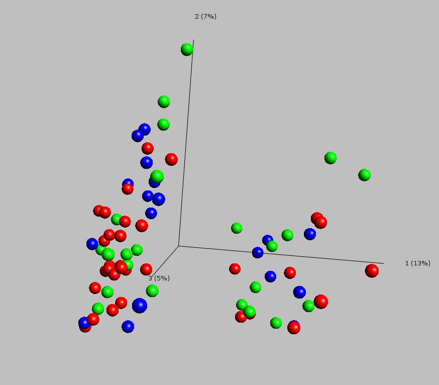
The first three principal components contain of the total variance in the dataset and so for this -D projection . Using randomization we estimate the expected value for a corresponding dataset (i.e. a dataset containing the same number of samples and variables) built on independent and normally distributed variables to be approximately . We have thus captured around times more variation than what we would have expected if the variables were independent and normally distributed. This indicates that we do have strong signals present in the dataset.
-
•
Following our exploration scheme we now look for possible outliers and artifacts.
The projected subjects are colored according to smoking history, but it is clear from Figure 1 that most of the variance in the first principal component (containing of the total variance in the data) comes from a signal that has a very weak association with smoking history. We nevertheless see a clear splitting into two subgroups. Looking at supplied clinical annotations one can conclude that the two groups are not associated to gender, age or race traits. Instead one finds that all the subjects in one of the groups have low subject description numbers whereas all the subjects except one in the other group have high subject description numbers. In Figure 2 we have colored the subjects according to description number. This suspected artifact signal does not correspond to any in the dataset (Dataset GDS 534, NCBIs GEO) supplied clinical annotation. One can hypothesize that the description number could reflect for instance the order in which the samples were gathered and thus could be an artifact. Even if the two groups actually correspond to some interesting clinical variable, like disease state, that we should investigate separately, we will consider the splitting to be an artifact in our investigation. We are interested in using all the assembled data to look for genes that discriminate between current smokers and never smokers. We thus eliminate the suspected artifact by mean-centering the two main (artifact) groups. After elimination of the strong artifact signal, the first three principal components contain ”only” of the total variation.
-
•
Following our exploration scheme we filter the genes with respect to variance visually searching for a possibly informative three dimensional projection.
| Gene symbol | -value |
|---|---|
| NQO1 | 5.59104067771824e-08 |
| GPX2 | 2.31142232391279e-07 |
| ALDH3A1 | 2.31142232391279e-07 |
| CLDN10 | 3.45691439169953e-06 |
| FTH1 | 4.72936617815058e-06 |
| TALDO1 | 4.72936617815058e-06 |
| TXN | 4.72936617815058e-06 |
| MUC5AC | 3.77806345774405e-05 |
| TSPAN1 | 4.50425200297664e-05 |
| PRDX1 | 4.58227420582093e-05 |
| MUC5AC | 4.99131989472012e-05 |
| AKR1C2 | 5.72678146958168e-05 |
| CEACAM6 | 0.000107637125805187 |
| AKR1C1 | 0.000195523829628407 |
| TSPAN8 | 0.000206106293159401 |
| AKR1C3 | 0.000265342898771159 |
| Gene symbol | -value |
|---|---|
| MT1G | 4.03809377378893e-07 |
| MT1X | 4.72936617815058e-06 |
| MUC5B | 2.38198903402317e-05 |
| CD81 | 3.1605221864278e-05 |
| MT1L | 3.1605221864278e-05 |
| MT1H | 3.1605221864278e-05 |
| SCGB1A1 | 4.50425200297664e-05 |
| EPAS1 | 4.63861480935914e-05 |
| FABP6 | 0.00017793865432854 |
| MT2A | 0.000236481909692626 |
| MT1P2 | 0.000251264650053933 |
When we filter down to the most variable genes, the three first principal components have an -projection content of , whereas by estimation using randomization we would have expected it to be . The projection in Figure 3 is thus probably informative. We have again colored the samples according to smoking history as above. The third principal component, containing of the total variance, can be seen to quite decently separate the current smokers from the never smokers. We note that this was impossible to achieve without removing the artifact signal since the artifact signal completely obscured this separation.
-
•
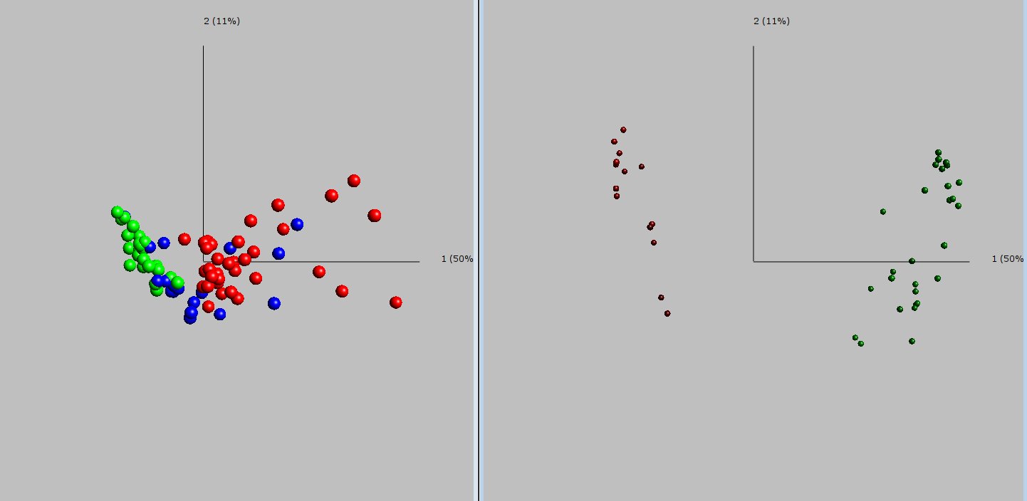
Using the variance filtered list of 630 genes as a basis, following our exploration scheme, we now perform a series of Student t-tests between the groups of current smokers and never smokers, i.e. different subjects.
For a specific level of significance we compute the -dimensional (i.e. we let ) -projection content resulting when we keep all the rejected null hypotheses, i.e. statistical discoveries. For a sequence of t-tests parameterized by the level of significance we now try to find a small level of significance and at the same time an observed -projection content with a large quotient compared to the expected projection content estimated by randomization. We supervise this procedure visually using three dimensional PCA-projections looking for visually clear patterns. For a level of significance of , leaving a total of genes (rejected nulls) and an FDR of we have whereas the expected projection content for randomized data . We have thus captured more than times of the expected projection content and at the same time approximately genes are false discoveries and so with high probability we have found potentially important biomarkers. We now visualize all subjects using these genes as variables. In Figure 4 we see a synchronized biplot with samples to the left and variables to the right. The sample plot shows a perfect separation of current smokers and never smokers. In the variable plot we see genes (green) that are upregulated in the current smokers group to the far right. The top genes according to -value for the Student t-test between current smokers and never smokers, that are upregulated in the current smokers group and downregulated in the never smokers group, are given in Table 3. In Table 4 we list the top genes that are downregulated in the current smokers group and upregulated among the never smokers.
7.2 Analysis of various muscle diseases.
In the study by Bakay et. al. [10] the authors studied 125 human muscle biopsies from 13 diagnostic groups suffering from various muscle diseases. The platforms used were Affymetrix U133A and U133B chips. The dataset can be downloaded from NCBIs Gene Expression Omnibus (DataSet GDS2855, accession no. GSE3307). We will analyze the dataset looking for phenotypic classifications and also looking for biomarkers for the different phenotypes.
-
•
We first use -dimensional PCA-projections of the samples of the data correlation matrix, filtering the genes with respect to variance and visually searching for clear patterns.
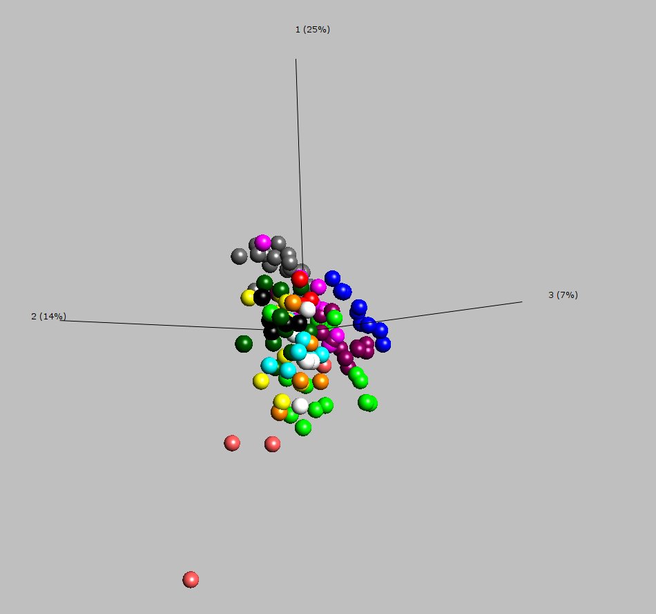
When filtering out the genes having most variability over the sample set we see several samples clearly distinguishing themselves and we capture of the total variance compared to the, by randomization estimated, expected . The plot in Figure 5 thus contains strong signals. Comparing with the color legend we conclude that the patients suffering from spastic paraplegia (Spg) contribute a strong signal. More precisely, three of the subjects suffering from the variant Spg-4 clearly distinguish themselves, while the remaining patient in the Spg-group suffering from Spg-7 falls close to the rest of the samples.
| Gene symbol | -value |
|---|---|
| RAB40C | 0.0000496417 |
| SFXN5 | 0.000766873 |
| CLPTM1L | 0.00144164 |
| FEM1A | 0.0018485 |
| HDGF2 | 0.00188435 |
| WDR24 | 0.00188435 |
| NAPSB | 0.00188435 |
| ANKRD23 | 0.00188435 |
-
•
We perform Student t-tests between the spastic paraplegia group and the normal group.
As before we now, in three dimensional PCA-projections, visually search for clearly distinguishable patterns in a sequence of Student t-tests parametrized by level of significance, while at the same time trying to obtain a small FDR. At a level of significance of , leaving a total of genes (rejected nulls) with an FDR of , the first three principal components capture of the variance compared to the, by randomization, expected . Table 5 lists the top genes upregulated in the group spastic paraplegia. We can add that these genes are all strongly upregulated for the three particular subjects suffering from Spg-4, while that pattern is less clear for the patient suffering from Spg-7.
-
•
In order to find possibly obscured signals, we now remove the Spastic paraplegia group from the analysis.
We also remove the Normal group from the analysis since we really want to compare the different diseases. Starting anew with the entire set of genes, filtering with respect to variance, we visually obtain clear patterns for the most variable genes. The first three principal components capture of the total variance compared to the, by randomization estimated, expected .
-
•
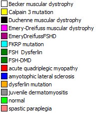
Using these most variable genes as a basis for the analysis, we now construct a graph connecting every sample with its two nearest (using euclidean distances in the -dimensional space) neighbors.
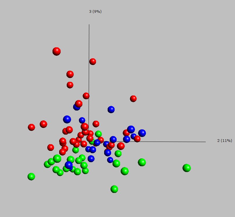
As described in the section on multidimensional scaling above, we now compute geodesic distances in the graph between samples, and construct a resulting distance (between samples) matrix. We then convert this distance matrix to a corresponding covariance matrix and finally perform a PCA on this covariance matrix. The resulting plot (together with the used graph) of the so constructed three dimensional PCA-projection is depicted in Figure 6.
Comparing with the Color legend in Figure 5, we clearly see that the groups juvenile dermatomyositis, amyotophic lateral sclerosis, acute quadriplegic myopathy and also Emery-Dreifuss FSHD distinguish themselves.
One should now go on using Student t-tests to find biomarkers (i.e. genes) distinguishing these different groups of patients, then eliminate these distinct groups and go on searching for more structure in the dataset.
7.3 Pediatric Acute Lymphoblastic Leukemia (ALL)
We will finally analyze a dataset consisting of gene expression profiles from 132 different patients, all suffering from some type of pediatric acute lymphoblastic leukemia (ALL). For each patient the expression levels of 22282 genes are analyzed. The dataset comes from the study by Ross et. al. [44] and the primary data are available at the St. Jude Children’s Research Hospital’s website [50]. The platform used to collect this example data set was Affymetrix HG-U133 chip, using the Affymetrix Microarray suite to select, prepare and normalize the data.
As before we start by performing an SVD on the data correlation matrix visually searching for interesting patterns and assessing the signal to noise ratio by comparing the actual -projection content in the real world data projection with the expected -projection content in corresponding randomized data.
-
•
We filter the genes with respect to variance, looking for strong signals.
In Figure 7 we see a plot of a three dimensional projection using the most variable genes as a basis for the analysis. We clearly see that the group T-ALL is mainly responsible for the signal resulting in the first principal component occupying of the total variance. In fact by looking at supplied annotations we can conclude that all of the other subjects in the dataset are suffering from B-ALL, the other main ALL type.
-
•
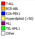
We now perform Student t-tests between the group T-ALL and the rest. We parametrize by level of significance and visually search for clear patterns.
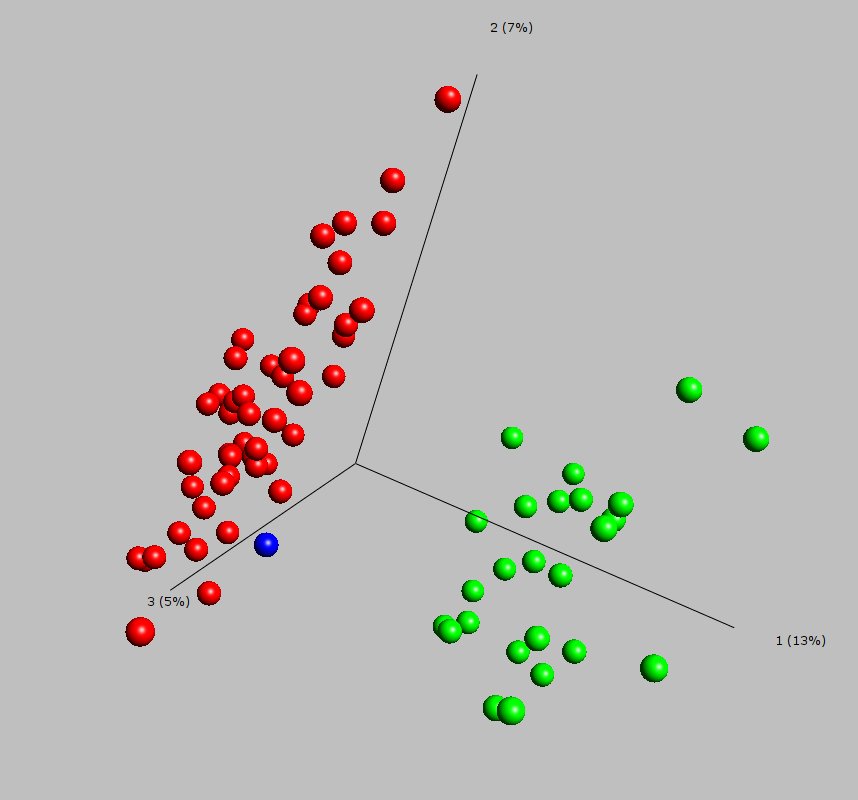
In Figure 8 we see a biplot based on the 70 genes that best discriminate between T-ALL and the rest. The FDR is extremely low telling us that with a very high probability the genes found are relevant discoveries. The most significantly upregulated genes in the T-ALL group are
CD3D, CD7, TRD@, CD3E, SH2D1A and TRA@.
The most significantly downregulated genes in the T-ALL group are
CD74, HLA-DRA, HLA-DRB, HLA-DQB and BLNK.
By comparing with gene-lists from the MSig Data Base (see [36]) we can see that the genes that are upregulated in the T-ALL group (CD3D, CD7 and CD3E) are represented in lists of genes connected to lymphocyte activation and lymphocyte differentiation.
-
•
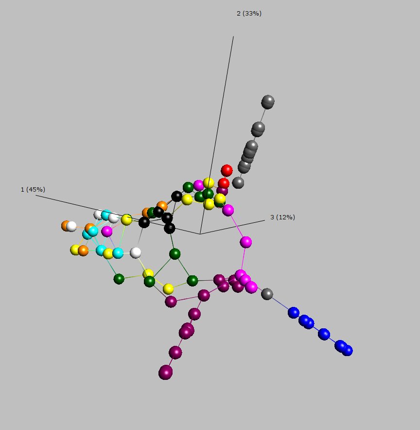
We now remove the group T-ALL from the analysis and search for visually clear patterns among three dimensional PCA-projections filtrating the genes with respect to variance.
Starting anew with the entire list of genes, filtering with respect to variance, a clear pattern is obtained for the most variable genes. We capture of the total variance as compared to the expected . We thus have strong signals present.
-
•
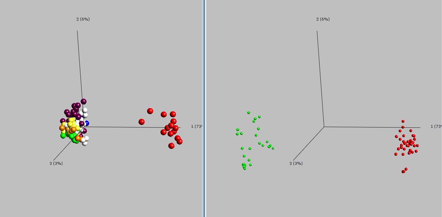
Using these most variable genes as a basis for the analysis, we now construct a graph connecting every sample with its two nearest neighbors.
We now perform the ISOMAP-algorithm with respect to this graph. The resulting plot (together with the used graph) of the so constructed three dimensional PCA-projection is depicted in Figure 9. We can clearly distinguish the groups E2A-PBX1, MLL and TEL-AML1. The group TEL-AML1 is connected to a subgroup of the group called Other. This subgroup actually corresponds to the Novel Group discovered in the study by Ross et.al. [44]. Note that by using ISOMAP we discovered this Novel subgroup only by variance filtering the genes showing that ISOMAP is a useful tool for visually supervised clustering.
Acknowledgement I dedicate this review article to Professor Gunnar Sparr. Gunnar has been a role model for me, and many other young mathematicians, of a pure mathematician that evolved into contributing serious applied work. Gunnar’s help, support and general encouragement have been very important during my own development within the field of mathematical modeling. Gunnar has also been one of the ECMI pioneers introducing Lund University to the ECMI network.
I sincerely thank Johan Råde for helping me to learn almost everything I know about data exploration. Without him the here presented work would truly not have been possible. Applied work is best done in collaboration and I am blessed with Thoas Fioretos as my long term collaborator within the field of molecular biology. I am grateful for what he has tried to teach me and I hope he is willing to continue to try. Finally I thank Charlotte Soneson for reading this work and, as always, giving very valuable feed-back.
Keywords: multivariate statistical analysis, principal component analysis, biplots, multidimensional scaling, multiple hypothesis testing, false discovery rate, microarray, bioinformatics
References
- [1] O. Alter, P. Brown, D. Botstein Singular value decomposition for genome-wide expression data processing and modeling. Proceedings of the National Academy of Science 97 (18), (2000) pp. 10101–10106.
- [2] T.W. Anderson Asymptotic theory for principal component analysis Ann. Math. Statist. 34, (1963) pp 122–148.
- [3] T. W. Anderson An introduction to multivariate statistical analysis. 3rd ed. (2003), Wiley, Hoboken, NJ.
- [4] The European Bioinformatics Institute’s database ArrayExpress: http://www.ebi.ac.uk/microarray-as/ae/
- [5] M. Ashburner et.al. The Gene Ontolgy Consortium. Gene Ontology: tool for the unification of biology. Nat. Genet. 25, (2000), pp. 25–29.
- [6] R. Autio et. al. Comparison of Affymetrix data normalization methods using 6,926 experiments across five array generations. BMC Bioinformatics Vol. 10, suppl.1 S24 (2009).
- [7] Z. D. Bai Methodologies in spectral analysis of large dimensional random matrices, A review. Stat. Sinica 9 (1999) pp. 611–677.
- [8] E. Bair, R. Tibshirani Semi-supervised methods to predict patient survival from gene expression data. PLOS Biology 2, (2004), pp. 511–522.
- [9] E. Bair, T. Hastie, D. Paul, R. Tibshirani Prediction by supervised principle components. J. Amer. Stat. Assoc. 101, (2006), pp. 119–137.
- [10] M. Bakay et al. Nuclear envelope dystrophies show a transcriptional fingerprint suggesting disruption of Rb-MyoD pathways in muscle regeneration. Brain (2006), 129(Pt 4), pp. 996-1013.
- [11] W.T. Barry, A.B. Nobel, F.A. Wright A statistical framework for testing functional categories in microarray data. The Annals of Appl. Stat. Vol. 2, No 1, (2008), pp. 286–315.
- [12] Y. Benjamini, Y. Hochberg Controlling the false discovery rate: a practical and powerful approach to multiple testing J. R. Stat. Soc. Ser. B, 57, (1995) pp. 289–300.
- [13] Y. Benjamini, Y. Hochberg On the adaptive control of the false discovery rate in multiple testing with independent statistics. J. Edu. Behav. Stat., 25, (2000), pp. 60–83.
- [14] Y. Benjamini, D. Yekutieli The control of the false discovery rate in multiple testing under dependency. The Annals of Statistics, 29,(2001), pp. 1165–1188.
- [15] C. J.F. Ter Braak Interpreting canonical correlation analysis through biplots of structure correlations and weights. Psychometrika Vol. 55, No 3 (1990) pp. 519–531.
- [16] X. Chen, L. Wang, J.D. Smith, B. Zhang Supervised principle component analysis for gene set enrichment of microarray data with continuous or survival outcome. Bioinformatics Vol 24, no 21, (2008) pp. 2474–2481.
- [17] P. Debashis, E. Bair, T. Hastie, R. Tibshirani ”Preconditioning” for feature selection and regression in high-dimensional problems. The Annals of Statistics, Vol. 36, No 4, (2008), pp. 1595–1618.
- [18] P. Diaconis Patterns in eigenvalues: The 70 th Josiah Willard Gibbs Lecture. Bulletin of the AMS Vol. 40, No 2 (2003) pp. 155–178.
- [19] National Centre for Biotechnology Information’s database Gene Expression Omnibus (GEO): http://www.ncbi.nlm.nih.gov/geo/
- [20] K. R. Gabriel The biplot graphic display of matrices with application to principal component analysis. Biometrika 58, (1971) pp. 453–467.
- [21] K.R. Gabriel Biplot. In S. Kotz; N.L. Johnson (Eds.) Encyclopedia of Statistical Sciences Vol 1 (1982) New York; Wiley pp. 263–271.
- [22] J.C. Gower, D.J. Hand Biplots. Monographs on Statistics and Applied probability 54; Chapman & Hall; London (1996).
- [23] H. Hotelling The generalization of Student’s ratio, Ann. Math. Statist. (1931), Vol. 2, pp 360 -378.
- [24] H. Hotelling Analysis of a complex of statistical variables into principal components. J. Educ. Psychol. 24, (1933), pp 417–441; pp 498–520.
- [25] K. Pearson On lines and planes of closest fit to systems of points in space. Phil. Mag. (6), 2, (1901), pp 559–572.
- [26] I. M. Johnstone On the distribution of the largest eigenvalue in Principle Components Analysis. Ann. of Statistics Vol 29, No 2 (2001) pp. 295–327.
- [27] I. M. Johnston High dimensional statistical inference and random matrices. Prooc. of the Intern. congress of Math, Madrid, Spain 2006, (EMS 2007).
- [28] M. Kanehisa, S. Goto KEGG:Kyoto Encyclopedia of Genes and Genomes. Nucleic Acids Res. 28, (2000), pp. 27–30.
- [29] K. Karhunen, Über lineare Methoden in der Wahrscheinlichkeitsrechnung, Ann. Acad. Sci. Fennicae. Ser. A. I. Math.-Phys., No 37, (1947), pp. 1 79.
- [30] N. El Karoui Spectrum estimation for large dimensional covariance matrices using random matrix theory. The Ann. of Statistics Vol 36, No 6 (2008) pp. 2757–2790.
- [31] P. Khatri, S. Draghici, Ontological analysis of gene expression data: current tools, limitations, and open problems. Bioinformatics, Vol. 21, no 18, (2005), pp. 3587–3595.
- [32] B.S. Kim et. al. Statistical methods of translating microarray data into clinically relevant diagnostic information in colorectal cancer. Bioinformatics, 21, (2005), pp. 517–528.
- [33] S.W. Kong, T.W. Pu, P.J. Park A multivariate approach for integrating genome-wide expression data and biological knowledge. Bioinformatics Vol. 22, no 19, (2006), pp. 2373–2380.
- [34] M. Loève, Probability theory. Vol. II, 4th ed., Graduate Texts in Mathematics, Vol. 46, Springer-Verlag, 1978, ISBN 0-387-90262-7.
- [35] L. Mirsky Symmetric gauge functions and unitarily invariant norms. The quarterly journal of mathematics Vol 11 No 1 (1960) pp. 50–59.
- [36] The Broad Institute’s Molecular Signatures Database (MSigDB): http://www.broadinstitute.org/gsea/msigdb/
- [37] V. K. Mootha et. al. Pgc-1 alpha-responsive genes involved in oxidative phosphorylation are coordinately downregulated in human diabetes Nat. Genet. 34, (2003), pp 267–273.
- [38] J. Nilsson, T. Fioretos, M. Höglund, M. Fontes Approximate geodesic distances reveal biologically relevant structures in microarray data. Bioinformatics Vol. 20, no 6, (2004), pp 874–880.
- [39] Y. Pawitan, S. Michiels, S. Koscielny, A. Gusnanto and A. Ploner False discovery rate, sensitivity and sample size for microarray studies Bioinformatics Vol. 21 no. 13 (2005), pp. 3017 -3024.
- [40] C. R. Rao Separation theorems for singular values of matrices and their applications in multivariate analysis. J. of Multivariate analysis 9 (1979) pp. 362–377.
- [41] D. Rasch, F. Teuscher, V. Guiard How robust are tests for two independent samples? Journal of statistical planning and inference 137 (2007) pp. 2706–2720.
- [42] I. Rivals, L. Personnaz, L. Taing, M-C Potier Enrichment or depletion of a GO category within a class of genes: which test? Bioinformatics Vol. 23, no 4, (2007), pp. 401–407.
- [43] D.M. Rocke, T. Ideker, O. Troyanskaya, J. Queckenbush, J. Dopazo Editorial note: Papers on normalization, variable selection, classification or clustering of microarray data Bioinformatics Vol. 25, no 6, (2009), pp. 701–702.
- [44] M.E. Ross et. al. Classification of pediatric acute lymphoblastic leukemia by gene expression profiling Blood 15 October 2003, Vol 102, No 8, pp 2951–2959.
- [45] Qlucore Omics Explorer, Qlucore AB, www.qlucore.com
- [46] A. Spira et al. Effects of Cigarette Smoke on the Human Airway Epithelial Cell Transcriptome Proceedings of the National Academy of Sciences, Vol. 101, No. 27 (Jul. 6, 2004), pp. 10143-10148.
- [47] G.W. Stewart On the early history of the singular value decomposition SIAM Review, Vol 35, no 4 (1993) pp. 551–566.
- [48] J.D. Storey A direct approach to false discovery rates. J.R. Stat. Soc. Ser. B, 64, (2002), pp. 479–498.
- [49] J. D. Storey, R. Tibshirani Statistical significance for genomewide studies. Proc. Natl. Acad. Sci. USA, 100, (2003), pp. 9440–9445.
- [50] St. Jude Children’s Research Hospital: http://www.stjuderesearch.org/data/ALL3/index.html
- [51] A. Subramanian et.al. Gene set enrichment analysis: a knowledgebased approach for interpreting genome wide expression profiles. Proc. Natl. Acad. Sci. USA, 102, (2005) pp. 15545–15550.
- [52] J. B. Tenenbaum, V. de Silva and J. C. Langford A Global Geometric Framework for Nonlinear Dimensionality Reduction. Science 290 (22 Dec. 2000): pp. 2319-2323.
- [53] O. Troyanskaya et. al. Missing value estimatin methods for DNA microarrays. Bioinformatics Vol. 17, no 6, (2001) pp. 520–525.
- [54] Y. Yin, C. E. Soteros, M.G. Bickis A clarifying comparison of methods for controlling the false discovery rate. Journal of statistical planning and inference 139 (2009) pp. 2126–2137.
- [55] Y. Q. Yin, Z. D. Bai, P.R. Krishnaiah On the limit of the largest eigenvalue of the large dimensional sample covariance matrix Probab. Theory Related Fields 78 (1988) pp. 509–521.