The maximum degree of planar graphs I. Series-parallel graphs

Abstract

We prove that the maximum degree $\Delta_{n}$ of a random series-parallel graph with $n$ vertices satisfies $\Delta_{n}/\log n\to c$ in probability, and $\mathbb{E}\,\Delta_{n}\sim c\log n$ for a computable constant $c>0$. The same result holds for outerplanar graphs.

1 Introduction

All graphs in this paper are simple and labelled. We recall that a graph is series-parallel if it does not contain the complete graph $K_{4}$ as a minor; equivalently, if it does not contain a subdivision of $K_{4}$. Since both $K_{5}$ and $K_{3,3}$ contain a subdivision of $K_{4}$, by Kuratowski’s theorem a series-parallel graph is planar. An outerplanar graph is a planar graph that can be embedded in the plane so that all vertices are incident to the outer face. They are characterized as those graphs not containing a minor isomorphic to (or a subdivision of) either $K_{4}$ or $K_{2,3}$; hence they form a subclass of series-parallel graphs.

In a previous paper [6] we determined the degree distribution in series-parallel graphs. More precisely, we showed that that the probability that a given vertex has degree $k$ in a random series-parallel graph with $n$ vertices tends to a computable constant $\overline{d}_{k}>0$ for all $k\geq 1$, as $n$ goes to infinity. In the present paper we use the ideas introduced in [6] and develop new techniques in order to study the maximum degree in random series-parallel graphs.

Our main result is the following. Let $\Delta_{n}$ denote the maximum degree of a random series-parallel graphs with $n$ vertices. Then

$$\frac{\Delta_{n}}{\log n}\to c\qquad\mbox{in probability}$$

and

$$\mathbb{E}\,\Delta_{n}\sim c\log n$$

for a certain constant $c>0$. The same result holds for 2-connected series-parallel graphs, and for outerplanar and 2-connected outerplanar graphs with suitable values of $c$. The constant $c$ is always well-defined analytically and can be computed as $c=1/\log(1/q)$, where $0<q<1$ is the exponential base in the asymptotic expansion of the corresponding degree distribution. We have

$$c \approx 3.482774\quad\mbox{for series-parallel graphs},$$

$$c \approx 1.035792\quad\mbox{for outerplanar graphs},$$

$$c \approx 3.679771\quad\mbox{for $2$-connected series-parallel graphs},$$

$$c \approx 1.134592\quad\mbox{for $2$-connected outerplanar graphs}.$$

This result was conjectured in [1] and, as we are going to see, is the natural result to expect in this context. McDiarmid and Reed [12] have recently proved that the maximum degree $\Delta_{n}$ in random planar graphs is of order $\Theta(\log n)$ with high probability; it is thus natural to expect that with high probability $\Delta_{n}\sim c\log n$ also in this case; this will be treated in a companion paper [7]. We remark that an analogous result holds for planar maps [10], counted according to the number of edges; in this case much more is know, since the authors obtain the full limit distribution of $\Delta_{n}$.

Intuitively the reason for the $\Delta_{n}\sim c\log n$ estimate is the following. Let $d_{n,k}$ denote the probability that a random vertex in a random planar graph of size $n$ has degree $k$. Then it is known (see [6]) that $d_{n,k}\to\overline{d}_{k}$ as $n\to\infty$, where $\overline{d}_{k}$ is a sequence of positive numbers that satisfy $\overline{d}_{k}\sim ck^{\alpha}q^{k}$ as $k\to\infty$ (for computable constants $c$ and $q$). Thus, we can expect that $d_{n,k}\approx ck^{\alpha}q^{k}$ holds for $n,k\to\infty$ (in a properly chosen range) and also

$$\sum_{\ell>k}d_{n,\ell}\approx\frac{cq}{1-q}k^{\alpha}q^{k}.$$

Furthermore, let $Y_{n,k}$ denote the random variable that counts the number of vertices of degree $>k$ in a random planar graph of size $n$. Then

$$\mathbb{E}\,Y_{n,k}=n\sum_{\ell>k}d_{n,\ell}\approx n\frac{cq}{1-q}k^{\alpha}q^{k},$$ (1.1)

and by definition

$$Y_{n,k}>0\quad\Longleftrightarrow\quad\Delta_{n}>k.$$

Hence the probability $\mathbb{P}\{\Delta_{n}>k\}=\mathbb{P}\{Y_{n,k}>0\}\leq\mathbb{E}\,Y_{n,k}$ is negligible if $nk^{\alpha}q^{k}\to 0$. Usually such a threshold is tight so that one can expect that the converse statement is also true, which implies $\Delta_{n}\sim c\log n$ for $c=1/\log(1/q)$.

In this paper we make this heuristics rigorous by applying the first and second moment method. The precise statement that we show is the following, which can be considered as a kind of Master Theorem for proving results on the maximum degree. The proof is based on standard techniques, and we present it in Appendix A.

Theorem 1.1.

Let $d_{n,k}$ denote the probability that a randomly selected vertex of a certain class of random graphs of size $n$ has degree $k$, and let $d_{n,k,\ell}$ denote the probability that two different randomly selected (ordered) vertices have degrees $k$ and $\ell$. Suppose that we have the following properties:

1. There exists a limiting degree distribution $\overline{d}_{k}$ ($k\geq 1$) with an asymptotic behaviour of the form

   $$\log\overline{d}_{k}\sim k\log q\qquad(k\to\infty),$$ (1.2)

   where $q$ is a real constant with $0<q<1$.

2. We have, as $n\to\infty$, $k\to\infty$, $\ell\to\infty$, and uniformly for $k,\ell\leq C\log n$ (for an arbitrary constant $C>0$)

   $$d_{n,k}\sim\overline{d}_{k}\quad\mbox{and}\quad d_{n,k,\ell}\sim\overline{d}_{k}\overline{d}_{\ell}.$$ (1.3)

3. There exists $\overline{q}<1$ such that, uniformly for all $n,k,\ell\geq 1$,

   $$d_{n,k}=O(\overline{q}^{k})\quad\mbox{and}\quad d_{n,k,\ell}=O(\overline{q}^{k+\ell}).$$ (1.4)

Let $\Delta_{n}$ denote the maximum degree of a random graph of size $n$ in this class. Then

$$\frac{\Delta_{n}}{\log n}\to\frac{1}{\log(1/q)}\qquad\mbox{in probability}$$ (1.5)

and

$$\mathbb{E}\,\Delta_{n}\sim\frac{1}{\log(1/q)}\,\log n\qquad(n\to\infty).$$ (1.6)

Condition 1 is fulfilled for planar, series-parallel and outerplanar graphs, as shown in [6]. Condition 2 is the key to applying the second moment method, as it gives access to the variance of the number of vertices of degree $k$. It can be viewed as a kind of asymptotic independence, in the sense that for random vertices $v_{1}$ and $v_{2}$, as $n\to\infty$ we have

$$\mathbb{P}(\deg(v_{1})=k,\deg(v_{2})=l)\sim\mathbb{P}(\deg(v_{1})=k)\,\mathbb{P}(\deg(v_{2})=l).$$

The last condition is purely technical and is usually easy to verify.

Most of the paper is devoted to showing that outerplanar and series-parallel graphs satisfy the conditions imposed by Theorem 1.1, the bulk of the work being on verifying condition 2. For each of the two classes of graphs, we compute first the associated counting generating functions from combinatorial decompositions: this is done in Sections 2 (outerplanar) and 4 (series-parallel). Then, we analyze the generating functions as functions of complex variables in order to obtain precise asymptotics for the probability that a vertex or a pair of vertices have given degrees: this is done in Sections 3 and 5. These sections make use of several technical lemmas whose proofs are based on the Cauchy integration formula of analytic functions in several variables. The proofs of these lemmas are given in Appendix B.

Before concluding this introduction, we present some technical preliminaries needed in the paper: first the combinatorics of generating functions and secondly some analytic considerations.

Generating functions.

We use the following notation. For a class of labelled graphs $\mathcal{G}$ having $g_{n}$ graphs with $n$ vertices, we use

$$G(x)=\sum_{n}g_{n}\frac{x^{n}}{n!}$$

to denote the exponential generating function of $\mathcal{G}$. A rooted graph is a graph with a distinguished, or marked, vertex. A double rooted graph is a graph with two marked vertices that are different (we cannot mark the same vertex twice) and distinguishable (there is a first root vertex and a second root vertex). For convenience, we assume that marked vertices are not labelled, and they do not contribute towards the size of the graph. Note that the derivatives of $G(x)$,

$$G^{\prime}(x)=\sum_{n\geq 1}ng_{n}\frac{x^{n-1}}{n!}=\sum_{n}g_{n+1}\frac{x^{n}}{n!},\qquad G^{\prime\prime}(x)=\sum_{n}g_{n+2}\frac{x^{n}}{n!},$$

can also be interpreted as the exponential generating functions of rooted and double rooted graphs in $\mathcal{G}$.

When rooting a graph, we are often interested in the degree of the marked vertices, so we introduce generating functions

$$G^{\bullet}(x,w)=\sum_{n,k}g^{\bullet}_{n}d_{n+1,k}\frac{x^{n}}{n!}w^{k},\qquad G^{\bullet\bullet}(x,w,t)=\sum_{n,k,\ell}g^{\bullet\bullet}_{n}d_{n+2,k,\ell}\frac{x^{n}}{n!}w^{k}t^{\ell}$$

to enumerate rooted and double rooted graphs of $\mathcal{G}$, where the exponent of variable $x$ counts the number of non-root vertices, the exponents of variables $w$ and $t$ count the degrees of the first and second root, and the numbers $d_{n,k}$ and $d_{n,k,\ell}$ are the probabilities that a randomly selected vertex (respectively, two randomly selected vertices) of a graph of $\mathcal{G}$ of size $n$ has degree $k$ (respectively, have degrees $k$ and $\ell$). Notice that with this terminology, the coefficient $g^{\bullet}_{n}d_{n+1,k}$ is precisely the number of rooted graphs with $n$ vertices and where the root has degree $k$, and similarly for $g^{\bullet\bullet}_{n}d_{n+2,k,\ell}$. Since it holds that

$$G^{\bullet}(x,1)=G^{\prime}(x),\qquad G^{\bullet\bullet}(x,1,1)=G^{\prime\prime}(x)$$

we see that $g^{\bullet}_{n}=g_{n+1}$ and $g^{\bullet\bullet}_{n}=g_{n+2}$.

For the sake of readability, we always use $B(x)$ and $C(x)$ to denote the generating functions of 2-connected and connected graphs of the class of graphs we are working with, and $d_{n,k}$ and $d_{n,k,\ell}$ to denote the associated probabilities; the context will always make clear which class of graphs we refer to.

Singularity analysis.

To obtain the asymptotic estimates for $d_{n,k}$ and $d_{n,k,l}$ as required by Theorem 1.1, we analyse the singularities of the corresponding generating functions. It turns out that all these generating functions share the same singularity structure, which we proceed to describe.

A power series of the square-root type is a power series $y(x)$ with a square root singularity at $x_{0}>0$, that is, $y(x)$ admits a local representation of the form

$$y(x)=g(x)-h(x)\sqrt{1-x/x_{0}}$$ (1.7)

for $|x-x_{0}|<\varepsilon$ for some $\varepsilon>0$ and $|\arg(x-x_{0})|>0$, where $g(x)$ and $h(x)$ are analytic and non-zero at $x_{0}$. Moreover, $y(x)$ can be analytically continued to the region

$$D=D(x_{0},\varepsilon)=\{x\in\mathbb{C}:|x|<x_{0}+\varepsilon\}\setminus[x_{0},\infty).$$

Note that $y(x)$ can be represented alternatively as a power series in $X=\sqrt{1-x/x_{0}}$,

$$y(x)=a_{0}+a_{1}X+a_{2}X^{2}+a_{3}X^{3}+\cdots$$

for $|X|<\varepsilon^{1/2}$.

We illustrate the common singularity structure of our generating functions by using the explicit expression of the generating function of rooted 2-connected outerplanar graphs,

$$B^{\bullet}(x,w)=xw+{xw^{2}\over 2}{y(x)\over 1-y(x)w},$$ (1.8)

to be derived in Lemma 2.1, where $y(x)$ is an explicit power series of the square-root type. Clearly, $B^{\bullet}(x,w)$ has two possible sources of singularities: the square-root singularity of $y(x)$ at $x=x_{0}$, and the vanishing of the denominator $1-y(x)w$ at $w=1/y(x)$. These two sources coalesce at the critical point $x=x_{0},w=1/y(x_{0})$ (equivalently, $w=1/g(x_{0})$ due to the local representation $y(x)=g(x)-h(x)X$). We derive asymptotic estimates for $d_{n,k}$ with $n,k\rightarrow\infty$, on the range $k\leq C\log n$ for any $C>0$, by using multivariate Cauchy coefficient extraction on $B^{\bullet}(x,w)$ with an integration path close to the critical point $(x,w)=(x_{0},1/g(x_{0}))$. More precisely, we integrate along Hankel contours, following Flajolet and Odlyzko’s transfer theorems [8].

As for the remaining generating functions, they do not admit explicit expressions as $B^{\bullet}(x,w)$, but they share the same singularity structure: the square-root singularity of $y(x)$, and the vanishing of a term $1-y(x)w$. Curiously enough, the nature of the singularity induced by $1-y(x)w=0$ is different from case to case. This fact justifies the need of distinct but closely related technical lemmas tailored to the particular shapes of the generating functions. To wit, these singularities are poles and double poles for 2-connected outerplanar graphs (Lemmas 3.1 and 3.2), an essential singularity $e^{\infty}$ for connected outerplanar graphs (Lemmas 3.3 and 3.4, whose proofs make use of Hayman’s method [11] to obtain the asymptotics), and powers of square-roots for 2-connected and connected series-parallel graphs (Lemmas 5.3 and 5.4).

2 Outerplanar graphs: combinatorics

In this section we study the combinatorics of rooted and double rooted outerplanar graphs with respect to the degree of the roots. We obtain explicit or nearly explicit expressions for the corresponding generating functions, both for the case of 2-connected and connected outerplanar graphs. The analysis of their singularities is done later in Section 3, where we also state the main results on the maximum degree of outerplanar graphs.

2.1 $2$-Connected Outerplanar Graphs

Recall that an outerplanar graph is a planar graph that can be embedded in the plane so that all vertices are incident to the external face. Furthermore, $2$-connected outerplanar graphs are quite close to dissections. A dissection is a $(n+2)$-gon (with $n\geq 1$) where one edge is rooted and the vertices are connected inside it by means of diagonals that do not cross.

Let $A(x)$ denote the generating function of dissections with $n+2$ vertices, that is, the two vertices of the root edge are not counted. Then $A(x)$ is determined by the system

$$A(x) =(1+A(x))\,x\,S(x),$$

$$S(x) =(1+A(x))(1+xS(x)),$$

where the generating function $S(x)$ enumerates non-empty chains of dissections and single edges, the root edges are lined up, and the two vertices of the chain (the two poles of the network) are not counted (see Figure 1). Note that the term $1$ in $1+A(x)$ denotes the graph consisting of a single edge (which is not a dissection) while the term $1$ in $1+xS(x)$ denotes the empty chain.

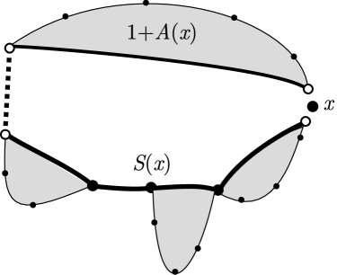
Figure 1: Closing a chain of dissections and edges to obtain a new dissection; the dashed edge is the new root edge.

This system can be solved explicitly and we find that $A(x)$ satisfies the quadratic equation

$$2xA^{2}+(3x-1)A+x=0$$

and is given by

$$A(x)={1-3x-\sqrt{1-6x+x^{2}}\over 4x}.$$ (2.1)

Observe that

$$S(x)=2A(x)+1={1-x-\sqrt{1-6x+x^{2}}\over 2x}.$$

Next we consider 2-connected labelled outerplanar graphs. There is exactly one 2-connected outerplanar graph with two vertices, namely a single edge. However, when $n\geq 3$ the number of 2-connected outerplanar graphs is

$$b_{n}=\frac{(n-1)!}{2}\,a_{n-2}.$$

To see this, note that $b_{n}$ coincides with the number $b^{\bullet}_{n-1}$ of rooted 2-connected outerplanar graphs on $n$ vertices with labels $1,2,\ldots,n-1$ (choose the vertex with label $n$ as root, and remove the label). Now consider a dissection with $n$ vertices, whose number is $a_{n-2}$. Direct the root edge of the dissection in counterclockwise order, and mark its first vertex. Then, there are exactly $(n-1)!$ ways to label the remaining $n-1$ vertices with $1,2,\ldots,n-1$. Finally, since the direction of the outer cycle is irrelevant, divide the resulting number $(n-1)!a_{n-2}$ by $2$ to get back $b_{n}$. Now, it is just a matter of computation to obtain that

$$B^{\prime}(x)=\sum_{n\geq 1}b_{n+1}\frac{x^{n}}{n!}=x+\frac{1}{2}xA(x)=\frac{1+5x-\sqrt{1-6x+x^{2}}}{8}.$$

Next we discuss the distribution of the degree of the first root in dissections. It will be easy to translate this into a corresponding result for $2$-connected outerplanar graphs. Let $A(x,w)$ be the generating function of dissections of an $(n+2)$-gon, where the exponent of $w$ counts the degree of the first vertex of the root edge. Similarly to the above we have

$$A(x,w)=w(w+A(x,w))\,x\,S(x),$$

and thus

$$A(x,w)=\frac{xw^{2}S(x)}{1-xS(x)}=\frac{xw^{2}(2A(x)+1)}{1-xw(2A(x)+1)}.$$

In this context we introduce for later use a generating function $S(x,w)$ that corresponds to series of dissections (compare with the above description) where the exponent of $w$ counts the degree of the first pole. Here we have

$$S(x,w)=(w+A(x,w))(1+xS(x)).$$

With the help of $A(x,w)$ we obtain an explicit representation for the generating function for rooted $2$-connected outerplanar graphs.

Lemma 2.1.

Let $B^{\bullet}(x,w)$ denote the bivariate generating function of labelled rooted $2$-connected outerplanar graphs, where the exponent of $x$ counts the number of non-root vertices and the exponent of $w$ counts the degree of the root vertex. Then we have

$$B^{\bullet}(x,w) =\sum_{n,k\geq 1}b_{n}^{\bullet}\,d_{n+1,k}\,\frac{x^{n}}{n!}\,w^{k}$$

$$=xw+\frac{1}{2}xA(x,w)$$

$$=xw+{xw^{2}\over 2}{x(2A(x)+1)\over 1-x(2A(x)+1)w},$$

where $b_{n}^{\bullet}=b_{n+1}$, and $d_{n+1,k}$ is the probability that a randomly selected vertex of a labelled 2-connected outerplanar graph of size $n+1$ has degree $k$.

Next we study double rooted 2-connected outerplanar graphs. As before, we start with dissections. Let $A_{1}(x,w,t)$ denote the generating function of dissections, where the exponents of $w$ and $t$ count the degree of the first and the second vertex of the root edge (in counterclockwise order). Similarly, we define $A_{2}(x,w,t)$ as the generating function of dissections $D$ with an additional root vertex $v$ not in the root edge, where the exponent of $w$ and $t$ count the degree of the first vertex of the root edge and the degree of $v$, respectively. We also introduce the generating function $S_{2}(x,w,t)$ for series of dissections with an additional root $v$ not in the poles, where the exponents of $w$ and $t$ count the degree of the first pole and the degree of $v$. Then we have the following relations:

$$A_{1}(x,w,t) =(w+A(x,w))wxtS(x,t)$$

$$A_{2}(x,w,t) =(wt+A_{1}(x,w,t))wxS(x,t)$$

$$+A_{2}(x,w,t)xwS(x)$$

$$+(w+A(x,w))xwS_{2}(x,1,t),$$

$$S_{2}(x,w,t) =A_{2}(x,w,t)(1+xS(x))$$

$$+(wt+A_{1}(x,w,t))xS(x,t)$$

$$+(w+A(x,w))xS_{2}(x,1,t).$$

The three summands for $A_{2}$ and $S_{2}$ correspond to the three places where the additional root $v$ can be placed: inside the first dissection, at the articulation vertex, or inside the series of dissections. Summing up, this yields

$$A(x,w) =\frac{xw^{2}(2A+1)}{1-xw(2A+1)},$$

$$S(x,w) =\frac{w(1+x(2A+1))}{1-xw(2A+1)},$$

$$A_{1}(x,w,t) =\frac{xw^{2}t^{2}(1+x(2A+1))}{(1-xw(2A+1))(1-xt(2A+1))}$$

$$A_{2}(x,1,t) =\frac{xt^{2}(1+x(2A+1))}{(1-xt(2A+1))^{2}(1-x(4A+3))}$$

$$S_{2}(x,1,t) =2\frac{xt^{2}(1+x(2A+1))}{(1-xt(2A+1))^{2}(1-x(4A+3))}$$

$$A_{2}(x,w,t) =\frac{xw^{2}t^{2}(1+x(2A+1))(P_{1}+x(wt-w-t)P_{2})}{(1-xw(2A+1))^{2}(1-xt(2A+1))^{2}(1-x(4A+3))},$$

where

$$P_{1} =1-x(4A+1),\qquad P_{2}=1-2A+x(2A+1).$$

Lemma 2.2.

Let $B^{\bullet\bullet}(x,w,t)$ denote the generating function of double rooted labelled $2$-connected outerplanar graphs, where the exponent of $x$ counts the number of non-root vertices, and the exponents of $w$ and $t$ count, respectively, the degree of the first and second root. Then we have

$$B^{\bullet\bullet}(x,w,t) =\sum_{n,k,\ell}b_{n}^{\bullet\bullet}\,d_{n+2,k,\ell}\,\frac{x^{n}}{n!}\,w^{k}\,t^{\ell}$$

$$=wt+\frac{1}{2}A_{1}(x,w,t)+\frac{1}{2}A_{2}(x,w,t)$$

$$=wt+\frac{x(1+x(2A+1)t^{2}w^{2}}{2(1-xw(2A+1))(1-xt(2A+1))}$$

$$+\frac{xw^{2}t^{2}(1+x(2A+1))(P_{1}+x(wt-w-t)P_{2})}{2(1-xw(2A+1))^{2}(1-xt(2A+1))^{2}(1-x(4A+3))},$$

where $b_{n}^{\bullet\bullet}=b_{n+2}$, and $d_{n+2,k,\ell}$ denotes the probability that two randomly selected vertices of a labelled 2-connected outerplanar graph of size $n+2$ have degrees $k$ and $\ell$.

2.2 Connected outerplanar graphs

We recall that in many classes of graphs, including outerplanar, series-parallel and planar graphs, a recursive relation holds between the generating functions $B(x)$ and $C(x)$ of $2$-connected and connected graphs, namely:

$$C^{\prime}(x)=e^{B^{\prime}(xC^{\prime}(x))}.$$ (2.2)

This follows from the block decomposition of a connected graph; see, for instance, [2]. This relation can be extended to the following one.

Lemma 2.3.

Let $C^{\bullet}(x,w)$ and $C^{\bullet\bullet}(x,w,t)$ be the generating functions of rooted and double rooted connected outerplanar graphs, where the exponents of $w$ and $t$ count the degree of the first and second root. Then, we have

$$C^{\bullet}(x,w)=e^{B^{\bullet}(xC^{\prime}(x),w)}$$

and

$$C^{\bullet\bullet}(x,w,t) =\frac{x}{(xC^{\prime}(x))^{\prime}}\frac{\partial}{\partial x}C^{\bullet}(x,w)\frac{\partial}{\partial x}C^{\bullet}(x,t)$$

$$+B^{\bullet\bullet}(xC^{\prime}(x),w,t)C^{\bullet}(x,w)C^{\bullet}(x,t).$$

Proof.

The equation for $C^{\bullet}(x,w)$ is the natural extension of Equation (2.2), since the degree of the root vertex is the sum of the degrees of the root vertices of the blocks incident to it.

Figure 2: Block decomposition of a connected graph with two roots, either sharing a common block (left), or not (right).

Next we consider double rooted graphs enumerated by $C^{\bullet\bullet}(x,w,t)$. Here we distinguish two situations, depending on whether the two roots are in the same block or not (see Figure 2). In the former case, we have a block with two roots, so a term $B^{\bullet\bullet}(x,w,t)$ appears. Each non-root vertex of this block is replaced by a rooted connected graph in $xC^{\prime}(x)$, while the second root is replaced by $C^{\bullet}(x,t)$, since this replacement contributes to the degree of the second root. Thus, the generating function of double rooted connected graphs where the two roots are in the same block is

$$e^{B^{\bullet}(xC^{\prime}(x),w)}B^{\bullet\bullet}(xC^{\prime}(x),w,t)C^{\bullet}(x,t).$$

If the roots are in different blocks, it is still true that one of the blocks incident to the first root is distinguished (the unique block leading to the second root), and so is one of its vertices (the articulation vertex leading to the second root). So this time the decomposition has a rooted block with an additional distinguished vertex, that is, a term $x\frac{\partial}{\partial x}B^{\bullet}(x,w)$. Every vertex is replaced by $xC^{\prime}(x)$, except for the distinguished one, which is replaced by $x\frac{\partial}{\partial x}C^{\bullet}(x,t)$, that is, a rooted connected graph with an additional root.

Hence, the generating function of $C^{\bullet\bullet}(x,w,t)$ is given by

$$C^{\bullet\bullet}(x,w,t) =e^{B^{\bullet}(xC^{\prime}(x),w)}x\frac{\partial}{\partial x}B^{\bullet}(xC^{\prime}(x),w)\frac{\partial}{\partial x}C^{\bullet}(x,t)$$

$$+e^{B^{\bullet}(xC^{\prime}(x),w)}B^{\bullet\bullet}(xC^{\prime}(x),w,t)C^{\bullet}(x,t)$$

$$=\frac{x}{(xC^{\prime}(x))^{\prime}}\frac{\partial}{\partial x}C^{\bullet}(x,w)\frac{\partial}{\partial x}C^{\bullet}(x,t)$$

$$+B^{\bullet\bullet}(xC^{\prime}(x),w,t)C^{\bullet}(x,w)C^{\bullet}(x,t).$$

∎

Note that in the outerplanar case the functions $C^{\bullet}(x,w)$ and $C^{\bullet\bullet}(x,w,t)$ are explicit in terms of $C^{\prime}(x)$. For example, we have

$$C^{\bullet}(x,w)=e^{xC^{\prime}(x)w+a(x)w^{2}/(1-wb(x))},$$ (2.3)

where

$$a(x) =\frac{1}{2}x^{2}C^{\prime}(x)^{2}(1+2A(xC^{\prime}(x))),$$

$$b(x) =xC^{\prime}(x)(1+2A(xC^{\prime}(x))).$$

This is due to the fact that we have an explicit expression for $B^{\bullet}(x,w)$, which is not true in general.

3 Outerplanar graphs: asymptotics

In this section we analyze the singularities of the multivariate generating functions derived in the previous section. By studying the “shape” of these functions when $x,w$ and $t$ get close to the relevant singularities we derive asymptotic estimates for the number $d_{n,k}$ and $d_{n,k,\ell}$, as $n,k,\ell\to\infty$ in a suitable range. By applying the Master Theorem discussed in the Introduction we obtain a precise estimate for the maximum degree of outerplanar graphs.

3.1 $2$-Connected Outerplanar Graphs

In Propositions 3.1 and 3.2 we obtain asymptotic estimates for the numbers $d_{n,k}$ and $d_{n,k,\ell}$.

Proposition 3.1.

Let $d_{n,k}$ denote the probability that a randomly selected vertex in a $2$-connected outerplanar graph with $n$ vertices has degree $k$. Then we have uniformly for $k\leq C\log n$

$$d_{n,k}=2k(\sqrt{2}-1)^{k}\left(1+O\left(\frac{1}{k}\right)\right).$$ (3.1)

Furthermore, we have uniformly for all $n,k\geq 1$

$$d_{n,k}=O(\overline{q}^{k})$$ (3.2)

for some real $\overline{q}$ with $0<\overline{q}<1$.

In order to prove the above result we need to perform singularity analysis on the generating function $B^{\bullet}(x,w)$ given in Lemma 2.1. The precise technical result we need is the following.

Lemma 3.1.

Let $f(x,w)=\sum_{n,k}f_{n,k}x^{n}w^{k}$ be a bivariate generating function of non-negative numbers $f_{n,k}$, and suppose that $f(x,w)$ can be represented as

$$f(x,w)=\frac{G(x,X,w)}{1-y(x)w},$$ (3.3)

where $X=\sqrt{1-x/x_{0}}$, $y(x)$ is a power series with non-negative coefficients of the square-root type as in (1.7),

$$y(x)=g(x)-h(x)\sqrt{1-x/x_{0}},$$

and the function $G(x,v,w)$ is analytic in the region

$$D^{\prime}=\{(x,v,w)\in\mathbb{C}^{3}:|x|<x_{0}+\eta,|v|<\eta,|w|<1/g(x_{0})+\eta\}$$

for some $\eta>0$, and satisfies $G(x_{0},0,1/g(x_{0}))\neq 0$.

Then we have uniformly for $k\leq C\log n$ (with an arbitrary constant $C>0$)

$$f_{n,k}=\frac{G(x_{0},0,1/g(x_{0}))h(x_{0})}{2\sqrt{\pi}}\,g(x_{0})^{k-1}x_{0}^{-n}k\,n^{-\frac{3}{2}}\left(1+O\left(\frac{1}{k}\right)\right).$$ (3.4)

Moreover, for every $\varepsilon>0$ we have uniformly for all $n,k\geq 0$

$$f_{n,k}=O\left((g(x_{0})+\varepsilon)^{k}x_{0}^{-n}n^{-\frac{3}{2}}\right).$$ (3.5)

If $g(x_{0})<1$, then $f_{n}=\sum_{k}f_{n,k}$ is given asymptotically by

$$f_{n}=\frac{1}{2\sqrt{\pi}}\left(\frac{h(x_{0})G(x_{0},0,1)}{(1-g(x_{0}))^{2}}-\frac{G_{v}(x_{0},0,1)}{1-g(x_{0})}\right)x_{0}^{-n}n^{-\frac{3}{2}}\left(1+O\left(\frac{1}{n}\right)\right),$$ (3.6)

and for every $k$ the limit

$$\overline{d}_{k}=\lim_{n\to\infty}\frac{f_{n,k}}{f_{n}}$$

exists.

The proof of Lemma 3.1 is given in Appendix B.

We proceed to prove Proposition 3.1. We remind the reader that the limit $\overline{d}_{k}=\lim_{n\to\infty}d_{n,k}$ exists for all fixed $k$, and that (see [6])

$$\overline{d}_{k}=2(k-1)(\sqrt{2}-1)^{k}.$$

Proof of Proposition 3.1.

Recall that the $d_{n,k}$ are encoded in the function $B^{\bullet}(x,w)$ (see Lemma 2.1). Next observe that $B^{\bullet}(x,w)$ has precisely the form of $f(x,w)$ in Lemma 3.1. In particular, we have that

$$y(x)=x(2A(x)+1)=\frac{1-x-\sqrt{1-6x+x^{2}}}{2}$$

is a power series with non-negative coefficients that admits the local expansion

$$y(x) =g(x)-h(x)\sqrt{1-\frac{x}{x_{0}}}$$

$$g(x) =\frac{1-x}{2}$$

$$h(x) =\frac{1}{2}\sqrt{1-xx_{0}},$$

with $x_{0}=3-2\sqrt{2}$, and that $G(x,X,w)$ is given by

$$G(x,X,w)=xw+\frac{xw}{4}\left(xw-w+x\sqrt{1-xx_{0}}X\right).$$

Hence, we just need to compute the evaluations

$$g(x_{0}) =\sqrt{2}-1$$

$$h(x_{0}) =\sqrt{3\sqrt{2}-4}$$

$$G(x_{0},0,1/g(x_{0})) =\frac{3-2\sqrt{2}}{2(\sqrt{2}-1)}$$

$$G(x_{0},0,1) =\frac{1}{2}(13-9\sqrt{2})$$

$$G_{v}(x_{0},0,1) =\frac{1}{2}(3-2\sqrt{2})\sqrt{3\sqrt{2}-4}$$

to obtain the asymptotics for $f_{n,k}$ and $f_{n}$, in accordance with Equations (3.4) and (3.6). Now it is just a matter of computation to check that

$$d_{n,k}=\frac{f_{n,k}}{f_{n}}=2k(\sqrt{2}-1)^{k}\left(1+O\left(\frac{1}{k}\right)\right),$$

as required by (3.1). Also, (3.2) follows immediately from (3.5). ∎

Next we turn to the case of double rooted graphs.

Proposition 3.2.

Let $d_{n,k,\ell}$ denote the probability that two different (and ordered) randomly selected vertices in a $2$-connected outerplanar graph with $n$ vertices have degrees $k$ and $\ell$. Then we have uniformly for $2\leq k,\ell\leq C\log n$

$$d_{n,k,\ell}=4k\ell\,(\sqrt{2}-1)^{k+\ell}\left(1+O\left(\frac{1}{k}+\frac{1}{\ell}\right)\right).$$ (3.7)

Furthermore, we have uniformly for all $n,k\geq 1$

$$d_{n,k,\ell}=O(\overline{q}^{k+\ell}),$$ (3.8)

for some real number $\overline{q}$ with $0<\overline{q}<1$.

Again we need a precise technical result, to be proved in Appendix B.

Lemma 3.2.

Let $f(x,w,t)=\sum_{n,k,\ell}f_{n,k,\ell}x^{n}w^{k}t^{\ell}$ be a triple generating function of non-negative numbers $f_{n,k,\ell}$, and assume that $f(x,w,t)$ can be represented as

$$f(x,w,t)=\frac{G(x,X,w,t)}{X\,(1-y(x)w)^{2}(1-y(x)t)^{2}},$$ (3.9)

where $X=\sqrt{1-x/x_{0}}$, $y(x)$ is a power series of the square-root type as in (1.7), and $G(x,v,w,t)$ is non-zero and analytic at $(x,0,w,t)=(x_{0},0,1/g(x_{0}),1/g(x_{0}))$.

Then we have uniformly for $k,\ell\leq C\log n$ (with an arbitrary constant $C>0$)

$$f_{n,k,\ell}=\frac{G(x_{0},0,1/g(x_{0}),1/g(x_{0}))}{\sqrt{\pi}}\,g(x_{0})^{k+\ell}x_{0}^{-n}k\,\ell\,n^{-\frac{1}{2}}\left(1+O\left(\frac{1}{k}+\frac{1}{\ell}\right)\right).$$

Moreover, for every $\varepsilon>0$ we have uniformly for all $n,k\geq 0$

$$f_{n,k,\ell}=O\left((g(x_{0})+\varepsilon)^{k+\ell}x_{0}^{-n}n^{-\frac{1}{2}}\right).$$ (3.10)

If $g(x_{0})<1$, then $f_{n}=\sum_{k,\ell}f_{n,k,\ell}$ is given asymptotically by

$$f_{n}=\frac{G(x_{0},0,1,1)}{\sqrt{\pi}(1-g(x_{0}))^{4}}x_{0}^{-n}n^{-\frac{1}{2}}\left(1+O\left(\frac{1}{n}\right)\right)$$

and for every pair $(k,\ell)$ the limit

$$d_{k,\ell}=\lim_{n\to\infty}\frac{f_{n,k,\ell}}{f_{n}}$$

exists.

Proof of Proposition 3.2.

Recall that $d_{n,k,\ell}$ are encoded in the function $B^{\bullet\bullet}(x,w,t)$, which is given explicitly in Lemma 2.2. The result follows from a direct application of Lemma 3.2, since $B^{\bullet\bullet}(x,w,t)$ is exactly of the form $f(x,w,t)$, with the same $y(x)=x(2A(x)+1)$ and $x_{0}=3-2\sqrt{2}$, as in the proof of Lemma 3.1. Indeed, the factors $(1-xw(2A+1))^{2}$ and $(1-xt(2A+1))^{2}$ in the denominator of $B^{\bullet\bullet}(x,w,t)$ become $(1-y(x)w)^{2}$ and $(1-y(x)t)^{2}$ in $f(x,w,t)$, and the factor $(1-x(4A+3))$ transforms into $\sqrt{1-xx_{0}}X$ (the term $\sqrt{1-xx_{0}}$ is analytic and contributes to $G(x,X,w,t)$).

We just need to compute the evaluations

$$G(x_{0},0,1/g(x_{0}),1/g(x_{0})) =\dfrac{\sqrt{2}}{2\sqrt{3\sqrt{2}-4}}$$

$$G(x_{0},0,1,1) =\dfrac{\sqrt{2}(\sqrt{2}-1)^{4}}{2\sqrt{3\sqrt{2}-4}}$$

$$(1-g(x_{0}))^{4} =(2-\sqrt{2})^{4}$$

and check that

$$\dfrac{G(x_{0},0,1/g(x_{0}),1/g(x_{0}))}{G(x_{0},0,1,1)(1-g(x_{0}))^{4}}=4.$$

Hence,

$$d_{n,k,\ell} =\frac{f_{n,k,\ell}}{f_{n}}=4k\ell(\sqrt{2}-1)^{k+\ell}\left(1+O\left(\frac{1}{k}+\frac{1}{\ell}\right)\right),$$

as required by (3.7). Also, (3.8) follows immediately from (3.10).

∎

Theorem 3.1.

Let $\Delta_{n}$ denote the maximum degree of a random labelled $2$-connected outerplanar graph with $n$ vertices. Then

$$\frac{\Delta_{n}}{\log n}\to\frac{1}{\log(\sqrt{2}+1)}\qquad\mbox{in probability}$$

and

$$\mathbb{E}\,\Delta_{n}\sim\frac{\log n}{\log(\sqrt{2}+1)}\qquad(n\to\infty).$$

Proof.

The proof is an application of Theorem 1.1 to the class of 2-connected outerplanar graphs. Condition 1 of the theorem is a direct consequence of either the asymptotics $\overline{d}_{k}\sim ck^{\alpha}q^{k}$ derived in [6], or the asymptotics from $d_{n,k}$ of Proposition 3.1. Conditions 2 and 3 follow from Proposition 3.1 (for the $d_{n,k}$), and Proposition 3.2 (for the $d_{n,k,\ell}$). The condition $d_{n,k,\ell}\sim\overline{d}_{k}\overline{d}_{\ell}$ is easily verified from both asymptotic estimates. ∎

Remark​​ .

Prior to the proof of Proposition 3.1, we mentioned that $\overline{d}_{k}=\lim_{n\to\infty}d_{n,k}=2(k-1)(\sqrt{2}-1)^{k}$. This relation can be verified easily by considering the generating function

$$\overline{p}(w)=\sum_{k\geq 2}\overline{d}_{k}w^{k}=\lim_{n\to\infty}\frac{[x^{n}]B^{\bullet}(x,w)}{[x^{n}]B^{\prime}(x)}.$$

By setting

$$H(x,w,z)=xw+{xw^{2}\over 2}{4z-3x\over 1-(4z-3x)w}$$

we have $B^{\bullet}(x,w)=H(x,w,B^{\prime}(x))$, and consequently, by [6, Lemma 3.1],

$$\overline{p}(w)=H_{z}(3-2\sqrt{2},w,B^{\prime}(3-2\sqrt{2}))=\frac{2w^{2}}{(1+\sqrt{2}-w)^{2}},$$

from where it follows the explicit expression for $\overline{d}_{k}$ for $k\geq 2$. Similarly we can analyze $B^{\bullet\bullet}(x,w,t)$. Define $\overline{d}_{k,\ell}=\lim_{n\to\infty}d_{n,k,\ell}$ and

$$\overline{p}(w,t)=\sum_{k,\ell\geq 2}\overline{d}_{k,\ell}w^{k}t^{\ell}=\lim_{n\to\infty}\frac{[x^{n}]B^{\bullet\bullet}(x,w,t)}{[x^{n}]B^{\prime\prime}(x)}.$$

The analytic situation is a little bit different from the univariate one. The asymptotic leading term comes from the factor $1/(1-x(4A+3))=1/\sqrt{1-6x+x^{2}}$. Hence it follows that

$$\overline{p}(w,t) =\left[\dfrac{\dfrac{xw^{2}t^{2}(1+x(2A+1))(P_{1}+x(wt-w-t)P_{2})}{2(1-xw(2A+1))^{2}(1-xt(2A+1))^{2}}}{\dfrac{x(1+x(2A+1))(P_{1}-xP_{2})}{2(1-x(2A+1))^{2}(1-x(2A+1))^{2}}}\right]_{x=3-2\sqrt{2},A=1/\sqrt{2}}$$

$$=\frac{2w^{2}}{(1+\sqrt{2}-w)^{2}}\frac{2t^{2}}{(1+\sqrt{2}-t)^{2}}=\overline{p}(w)\overline{p}(t).$$

It particular it follows that $\overline{d}_{k,\ell}=\overline{d}_{k}\overline{d}_{\ell}$ for all $k,\ell\geq 2$. The interpretation of this relation is that the degrees of the two randomly chosen vertices are independent in the limit (which is not unexpected). Furthermore, this relation provides an automatic proof that $d_{n,k,\ell}\sim\overline{d}_{k}\overline{d}_{\ell}$.

3.2 Connected Outerplanar Graphs

Again we need asymptotic expansions for $d_{n,k}$ and $d_{n,k,\ell}$, but in this case it is a little more involved due to the presence of essential singularities in the associated generating functions. We recall that $C^{\bullet}(x,w)$ and $C^{\bullet\bullet}(x,w,t)$ are explicit in terms of $C^{\prime}(x)$.

The numbers $c_{n}$ of vertex labelled outerplanar graphs satisfy [2]

$$c_{n} =c\cdot n^{-\frac{5}{2}}\rho^{-n}n!\left(1+O\left(\frac{1}{n}\right)\right),$$

where $\rho=v_{0}e^{-B^{\prime}(v_{0})}\approx 0.136594$ is the radius of convergence of $C(x)$ and $v_{0}\approx 0.170765$ satisfies the equation $1=v_{0}B^{\prime\prime}(v_{0})$. Furthermore, $C^{\prime}(x)$ has a local representation of the form (1.7).

Proposition 3.3.

Let $d_{n,k}$ denote the probability that a randomly selected vertex in a connected outerplanar graph with $n$ vertices has degree $k$. Then we have as $n,k\to\infty$ and uniformly for $k\leq C\log n$

$$d_{n,k}\sim\overline{d}_{k},$$ (3.11)

where $\overline{d}_{k}$ denotes the asymptotic degree distribution of connected outerplanar graphs encoded by the generating function

$$\overline{p}(w) =\sum_{k\geq 1}\overline{d}_{k}w^{k}$$

$$=\rho\frac{v_{0}^{2}(2A(v_{0})+1)(2A(v_{0})+1+2v_{0}A^{\prime}(v_{0}))w^{2}}{2(1-v_{0}(2A(v_{0})+1)w)^{2}}$$

$$\qquad\times\exp\left(v_{0}w+\frac{v_{0}^{2}(2A(v_{0})+1)w^{2}}{2(1-v_{0}(2A(v_{0})+1)w)}\right)$$

and is given asymptotically by

$$\overline{d}_{k}\sim c_{1}k^{1/4}e^{c_{2}\sqrt{k}}q^{k},$$

where $c_{1}\approx 0.667187$, $c_{2}\approx 0.947130$.

Furthermore, we have uniformly for all $n,k\geq 1$

$$d_{n,k}=O(\overline{q}^{k}),$$ (3.12)

for some real $\overline{q}$ with $0<\overline{q}<1$.

The corresponding technical result needed to prove the previous proposition is the following.

Lemma 3.3.

Let $f(x,w)=\sum_{n,k}f_{n,k}x^{n}w^{k}$ be a bivariate generating function of non-negative numbers $f_{n,k}$, and assume that $f(x,w)$ can be represented as

$$f(x,w)=G(x,X,w)\exp\left(\frac{H(x,X,w)}{1-y(x)w}\right),$$ (3.13)

where $X=\sqrt{1-x/x_{0}}$, $y(x)$ is a power series of the square-root type as in (1.7), and the functions $G(x,v,w)$ and $H(x,v,w)$ are non-zero and analytic at $(x,v,w)=(x_{0},0,1/g(x_{0}))$.

Then we have uniformly for $k\leq C\log n$ (with an arbitrary constant $C>0$)

$$f_{n,k} =\frac{G\left(x_{0},0,\frac{1}{g(x_{0})}\right)h(x_{0})\,H\left(x_{0},0,\frac{1}{g(x_{0})}\right)^{\frac{1}{4}}}{4\pi}\,e^{\frac{1}{2}H(x_{0},0,1/g(x_{0}))-\frac{1}{g(x_{0})}H_{w}(x_{0},0,1/g(x_{0}))}$$

$$\qquad\times g(x_{0})^{k-1}x_{0}^{-n}k^{\frac{1}{4}}e^{2\sqrt{Hx_{0},0,1/g(x_{0}))\,k}}n^{-\frac{3}{2}}\left(1+O\left(\frac{1}{\sqrt{k}}\right)\right).$$

Moreover, for every $\varepsilon>0$ we have uniformly for all $n,k\geq 0$

$$f_{n,k}=O\left((g(x_{0})+\varepsilon)^{k}x_{0}^{-n}n^{-\frac{3}{2}}\right).$$

If $g(x_{0})<1$ then, $f_{n}=\sum_{k}f_{n,k}$ is given asymptotically by

$$f_{n} =\exp\left(\frac{H(x_{0},0,1)}{1-g(x_{0})}\right)\left(G(x_{0},0,1)\left(\frac{h(x_{0})H(x_{0},0,1)}{(1-g(x_{0}))^{2}}-\frac{H_{v}(x_{0},0,1)}{1-g(x_{0})}\right)-G_{v}(x_{0},0,1)\right)$$

$$\qquad\times x_{0}^{-n}n^{-\frac{3}{2}}\left(1+O\left(\frac{1}{n}\right)\right),$$

and for every $k$ the limit

$$\overline{d}_{k}=\lim_{n\to\infty}\frac{f_{n,k}}{f_{n}}$$

exists.

Proof of Proposition 3.3.

The existence of $\overline{d}_{k}$, the probability generating function $\overline{p}(w)$ encoding them, and the asymptotic expression $\overline{d}_{k}\sim c_{1}k^{1/4}e^{c2\sqrt{k}}q^{k}$, have been derived in [6]. It only remains to show the asymptotic relations (3.11) and (3.12); these will follow from an application of Lemma 3.3 to $f(x,w)=C^{\bullet}(x,w)$ with $x_{0}=\rho$, the radius of convergence of $C^{\prime}(x)$.

Indeed, recall from Equation (2.3) that $C^{\bullet}(x,w)$ is of the form

$$C^{\bullet}(x,w)=\exp\left(xC^{\prime}(x)w\right)\exp\left(\frac{a(x)w^{2}}{1-wb(x)}\right),$$

with

$$a(x) =\frac{1}{2}x^{2}C^{\prime}(x)^{2}(1+2A(xC^{\prime}(x))),$$

$$b(x) =xC^{\prime}(x)(1+2A(xC^{\prime}(x))).$$

Note that $C^{\prime}(x)$ is not analytic at $x=\rho$. Thus, we must use a local representation $C^{\prime}(x)=\overline{g}(x)-\overline{h}(x)\sqrt{1-x/\rho}$ of the form (1.7) in order to obtain the analytic expressions $A(x,v,w)$ and $G(x,v,w)$. In contrast with the 2-connected case, we are evaluating the function $A(x)$ at a point $\rho C^{\prime}(\rho)$ smaller that its radius of convergence $3-2\sqrt{2}$, so that both $A(xC^{\prime}(x))$ and

$$y(x)=b(x)=xC^{\prime}(x)\left(1+2A(xC^{\prime}(x))\right),$$

admit a local representation of the form (1.7).

Hence, we can apply Lemma 3.3 and deduce (3.11) and (3.12). Note that the asymptotic expansion for the $\overline{d}_{k}$ is derived from two sources, on the one side from asymptotic estimates on the coefficients of the PGF $\overline{p}(w)$, as in [6], and on the other side from the limit $f_{n,m}/f_{n}$ from Lemma 3.3. As expected, both asymptotic expansions coincide. ∎

The estimates for double rooted graphs come next, together with the associated technical result.

Proposition 3.4.

Let $d_{n,k,\ell}$ denote the probability that two different (and ordered) randomly selected vertices in a connected outerplanar graph with $n$ vertices have degrees $k$ and $\ell$. Then we have for $n,k,\ell\to\infty$ and uniformly for $2\leq k,\ell\leq C\log n$

$$d_{n,k,\ell}\sim\overline{d}_{k}\overline{d}_{\ell},$$ (3.14)

where $\overline{d}_{k}$ denotes the asymptotic degree distribution of connected outerplanar graphs. Furthermore, we have uniformly for all $n,k\geq 1$

$$d_{n,k,\ell}=O(\overline{q}^{k+\ell})$$ (3.15)

for some real $\overline{q}$ with $0<\overline{q}<1$.

Lemma 3.4.

Let $f(x,w,t)=\sum_{n,k,\ell}f_{n,k,\ell}x^{n}w^{k}t^{\ell}$ be a triple generating function of non-negative numbers $f_{n,k,\ell}$, and suppose that $f(x,w,t)$ can be represented as

$$f(x,w,t)=\frac{G(x,X,w,t)}{X}\frac{\exp\left(\frac{H(x,X,w)}{1-y(x)w}+\frac{H(x,X,t)}{1-y(x)t}\right)}{(1-y(x)w)^{2}(1-y(x)t)^{2}},$$ (3.16)

where $X=\sqrt{1-x/x_{0}}$, the functions $G(x,v,w,t)$ and $H(x,v,w)$ are non-zero and analytic at $(x,v,w,t)=(x_{0},0,1/g(x_{0}),1/g(x_{0}))$, and $y(x)$ is a power series of the square-root type as in (1.7).

Then we have uniformly for $k,\ell\leq C\log n$ (with an arbitrary constant $C>0$)

$$f_{n,k,\ell} =\frac{G(x_{0},0,1/g(x_{0}),1/g(x_{0})}{4\pi^{3/2}H(x_{0},0,1/g(x_{0}))^{3/2}}e^{H(x_{0},0,1/g(x_{0}))-\frac{2}{g(x_{0})}H_{w}(x_{0},0,1/g(x_{0}))}$$

$$\times g(x_{0})^{k+\ell}x_{0}^{-n}(k\ell)^{\frac{1}{4}}e^{2\sqrt{H(x_{0},0,1/g(x_{0})}(\sqrt{k}+\sqrt{\ell})}n^{-\frac{1}{2}}\left(1+O\left(\frac{1}{\sqrt{k}}+\frac{1}{\sqrt{\ell}}\right)\right).$$

Moreover, for every $\varepsilon>0$ we have uniformly for all $n,k\geq 0$

$$f_{n,k,\ell}=O\left((g(x_{0})+\varepsilon)^{k+\ell}x_{0}^{-n}n^{-\frac{1}{2}}\right).$$

If $g(x_{0})<1$, then $f_{n}=\sum_{k,\ell}f_{n,k,\ell}$ is given asymptotically by

$$f_{n}=\frac{G(x_{0},0,1,1)\exp\left(\frac{2H(x_{0},0,1)}{1-g(x_{0})}\right)}{\sqrt{\pi}(1-g(x_{0}))^{4}}\,x_{0}^{-n}n^{-\frac{1}{2}}\left(1+O\left(\frac{1}{n}\right)\right),$$

and for every pair $(k,\ell)$ the limit

$$d_{k,\ell}=\lim_{n\to\infty}\frac{f_{n,k,\ell}}{f_{n}}$$

exists.

Proof of Proposition 3.4.

As usual, we check that $C^{\bullet\bullet}(x,w,t)$ has the form of the generating function $f(x,w,t)$ in Lemma 3.4. Then (3.14) and (3.15) will follow automatically.

From (2.3) it follows that

$$\frac{\partial}{\partial x}C^{\bullet}(x,w)=e^{xC^{\prime}(x)w+a(x)w^{2}/(1-wb(x))}\left((xC^{\prime}(x))^{\prime}w+\frac{a^{\prime}(x)w^{2}}{1-wb(x)}+\frac{a(x)b^{\prime}(x)w^{3}}{(1-wb(x))^{2}}\right).$$

By using the local expansion of $C^{\prime}(x)$ it follows that $(xC^{\prime}(x))^{\prime}$, $a^{\prime}(x)$, and $b^{\prime}(x)$ can be represented as

$$\frac{\overline{g}(x)-\overline{h}(x)\sqrt{1-x/\rho}}{\sqrt{1-x/\rho}},$$

with functions $\overline{g}(x),\overline{h}(x)$ that are analytic and non-zero for $x=\rho$. Furthermore, observe that $B^{\bullet\bullet}(x,w,t)$ is analytic for $x=v_{0}=\rho C^{\prime}(\rho)$. Hence it follows easily that $C^{\bullet\bullet}(x,w,t)$ satisfies the assumptions of Lemma 3.4, as claimed. ∎

Theorem 3.2.

Let $\Delta_{n}$ denote the maximum degree of a random connected outerplanar vertex labelled graph with $n$ vertices. Then

$$\frac{\Delta_{n}}{\log n}\to c\qquad\mbox{in probability}$$

and

$$\mathbb{E}\,\Delta_{n}\sim c\,\log n\qquad(n\to\infty),$$

where $c=\displaystyle\frac{1}{\log(1/q)}$, and $q$ is given by

$$q=v_{0}\left(1+2A(v_{0})\right)\approx 0.380813,$$

and $v_{0}\approx 0.1707649$ satisfies the equation $1=v_{0}B^{\prime\prime}(v_{0})$.

Remark​​ .

Similarly as in the $2$-connected case, it is possible to check the relation $\overline{d}_{k,\ell}=\overline{d}_{k}\overline{d}_{\ell}$, or equivalently $\overline{p}(w,t)=\overline{p}(w)\overline{p}(t)$. However, in the connected case we can prove a more universal property. Suppose that we have a class of vertex labelled graphs whose block decomposition translates into the equation $C^{\prime}(x)=e^{B^{\prime}(xC^{\prime}(x))}$, and consequently into $C^{\bullet}(x,w)=e^{B^{\bullet}(xC^{\prime}(x),w)}$. Furthermore, assume that the radius of convergence of $B^{\prime}(x)$ is strictly larger than the evaluation of $xC^{\prime}(x)$ at its radius of convergence. Then we automatically have the property that $C^{\prime}(x)$ has a square-root singularity at its dominant singularty $\rho$ (which is also the radius of convergence). Setting $H(z,w)=e^{B^{\bullet}(z,w)}$, we have that (again by [6, Lemma 3.1])

$$\overline{p}(w)=\sum_{k\geq 1}\overline{d}_{k}w^{k}=H_{z}(\rho C^{\prime}(\rho),w)=e^{B^{\bullet}(\rho C^{\prime}(\rho),w)}\frac{\partial B^{\bullet}}{\partial x}(\rho C^{\prime}(\rho),w).$$

Next observe that the asymptotic leading part of $C^{\bullet\bullet}(x,w,t)$ comes from the term

$$T:=\frac{x}{(xC^{\prime}(x))^{\prime}}\frac{\partial}{\partial x}C^{\bullet}(x,w)\frac{\partial}{\partial x}C^{\bullet}(x,t).$$

Since

$$\frac{\partial}{\partial x}C^{\bullet}(x,w)=H_{z}(xC^{\prime}(x),w)(xC^{\prime}(x))^{\prime},$$

we also have

$$T=H_{z}(xC^{\prime}(x),w)H_{z}(xC^{\prime}(x),t)x(xC^{\prime}(x))^{\prime},$$

and consequently

$$\overline{p}(w,t)=\lim_{n\to\infty}\frac{[x^{n}]\,T}{[x^{n}]x(xC^{\prime}(x))^{\prime}}=H_{z}(\rho C^{\prime}(\rho),w)H_{z}(\rho C^{\prime}(\rho),t)=\overline{p}(w)\overline{p}(t).$$

In particular we obtain the relation $\overline{d}_{k,l}=\overline{d}_{k}\overline{d}_{\ell}$ for connected outerplanar graphs, as well as for connected series-parallel graphs.

4 Series-parallel graphs: combinatorics

We now turn our attention to the combinatorics of rooted and double rooted 2-connected and connected series-parallel graphs with respect to the degree of the roots. In this section we derive equations for the generating functions of these families of graphs, while their singularity analysis is postponed to Section 5.

4.1 SP networks

Recall that a connected series-parallel graph can be seen as the result of repeated series-parallel edge extensions applied to a tree. Thus, the basic element of a series-parallel graph is the result of series-parallel edge extensions of a single edge. Such graphs are also called series-parallel networks. They have two distinguished vertices (or roots) that are called poles. Series-parallel extensions induces a recursive description of SP networks: they are either a parallel composition of SP networks, a series composition of SP networks, or just the smallest network consisting of the two poles and an edge joining them.

Let $E(x)$ and $S(x)$ be the generating functions for labelled SP networks and series SP networks, where the exponent of $x$ counts the number of vertices other than the two poles. They satisfy the relations

$$E(x) =2e^{S(x)}-1,$$

$$S(x) =x(E(x)-S(x))E(x).$$

The first equation follows from the fact that a series SP network is a non-empty set of series SP networks (it is a parallel SP network if the set contains more than one network, and a series SP network otherwise), where the factor $2$ stands for choosing whether we have an edge joining both poles or not (see Figure 3). The second equation stablishes that a series SP network is always the series composition of two SP networks, where the first one is taken to be non-series to avoid multiple counting.

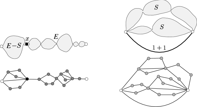
Figure 3: A parallel composition (left) and a series composition (right) of SP networks.

Next let $D(x,w)$ and $S(x,w)$ be the generating functions for SP and series SP networks, where the exponent of $w$ counts the degree of the first pole. Note that $E(x)=D(x,1)$ and $S(x)=S(x,1)$. (To be consistent, we should have chosen $D(x)$ instead of $E(x)$, but we have opted for $E(x)$ to avoid confusion in future formulas). Here we have

$$D(x,w) =(1+w)e^{S(x,w)}-1,$$

$$S(x,w) =x(D(x,w)-S(x,w))E(x).$$

We now consider double rooted SP networks: the first root is taken always as the first pole, while the second root is a vertex other than the first pole. Let $D_{1}(x,w,t)$ and $S_{1}(x,w,t)$ denote the generating functions for SP and series SP networks where the second root is the second pole, and $D_{2}(x,w,t)$ and $S_{2}(x,w,t)$ denote the generating functions for SP and series SP networks where the second root is not the second pole. Here, the exponents of $w$ and $t$ count the degree of the first and second root, respectively. The corresponding relations are

$$D_{1}(x,w,t) =(1+wt)e^{S_{1}(x,w,t)}-1,$$

$$S_{1}(x,w,t) =x(D(x,w)-S(x,w))D(x,t),$$

$$D_{2}(x,w,t) =(1+w)e^{S(x,w)}S_{2}(x,w,t),$$

$$S_{2}(x,w,t) =x(D_{2}(x,w,t)-S_{2}(x,w,t))E(x)$$

$$+x(D_{1}(x,w,t)-S_{1}(x,w,t))D(x,t)$$

$$+x(D(x,w)-S(x,w))D_{2}(x,1,t).$$

Note that $D(x,1)=D_{1}(x,1,1)=E(x)$, $S(x,1)=S_{1}(x,1,1)=S(x)$ and that $D_{2}(x,1,1)=xE^{\prime}(x)$ and $S_{2}(x,1,1)=xS^{\prime}(x)$. Also, observe that, by symmetry, $D_{1}(x,1,t)=D(x,t)$.

These equations can be easily solved. First one uses the implicit equation

$$E(x)=2\exp\left(\frac{xE(x)^{2}}{1+xE(x)}\right)-1$$ (4.1)

for $E(x)$ to express

$$S(x)=\frac{xE(x)^{2}}{1+xE(x)}.$$

Secondly, the implicit equation

$$D(x,w)=(1+w)\exp\left(\frac{xD(x,w)E(x)}{1+xE(x)}\right)-1$$ (4.2)

determines $D(x,w)$, and it can be used to obtain

$$S(x,w)=\frac{xE(x)}{1+xE(x)}D(x,w).$$

With the help of these representations we get directly

$$D_{1}(x,w,t) =(1+wt)\exp\left(\frac{x}{1+xE(x)}D(x,w)D(x,t)\right)-1,$$

$$S_{1}(x,w,t) =\frac{x}{1+xE(x)}D(x,w)D(x,t).$$

Next we set $w=1$ and obtain from the two equations for $D_{2}$ and $S_{2}$ the representations

$$D_{2}(x,1,t) =\frac{x(1+E(x))}{1-2xE(x)^{2}-x^{2}E(x)^{3}}D(x,t)^{2},$$

$$S_{2}(x,1,t) =\frac{x}{1-2xE(x)^{2}-x^{2}E(x)^{3}}D(x,t)^{2}.$$

Finally this gives

$$D_{2}(x,w,t) =\frac{x(1+D(x,w))D(x,t)}{1-xE(x)D(x,w)}\left((1+wt)\exp\left(\frac{x}{1+xE(x)}D(x,w)D(x,t)\right)-1\right)$$

$$+\frac{x^{2}E(x)(1+xE(x))}{1-2xE(x)^{2}-x^{2}E(x)^{3}}\frac{(1+D(x,w))D(x,w)D(x,t)^{2}}{1-xE(x)D(x,w)},$$

$$S_{2}(x,w,t) =\frac{xD(x,t)}{1-xE(x)D(x,w)}\left((1+wt)\exp\left(\frac{x}{1+xE(x)}D(x,w)D(x,t)\right)-1\right)$$

$$+\frac{x^{2}E(x)(1+xE(x))}{1-2xE(x)^{2}-x^{2}E(x)^{3}}\frac{D(x,w)D(x,t)^{2}}{1-xE(x)D(x,w)}.$$

4.2 $2$-connected SP graphs

It has been shown (see [6]) that the generating function $B(x)$ of $2$-connected SP graphs can be expressed in terms of $E(x)$ as

$$B(x)=\frac{1}{2}\log(1+xE(x))-\frac{xE(x)(x^{2}E(x)^{2}+xE(x)+2-2x)}{4(1+xE(x))}.$$ (4.3)

Next we recall that the generating function $B^{\bullet}(x,w)$ of rooted $2$-connected SP graphs, where the exponent of $x$ counts the number of non-root vertices and the exponent of $w$ the degree of the root, satisfies

$$w\frac{\partial}{\partial w}B^{\bullet}(x,w)=\sum_{k\geq 1}kB_{k}(x)w^{k}=xwe^{S(x,w)}.$$ (4.4)

From this relation it is possible to obtain an explicit representation for $B^{\bullet}(x,w)$.

Lemma 4.1 (From [6, Lemma 4.2]).

Let $B^{\bullet}(x,w)$ be the generating function of vertex rooted $2$-connected SP graphs, where the exponent of $x$ counts the number of vertices and the exponent of $w$ the degree of the root vertex. Then we have

$$B^{\bullet}(x,w)=x\left(D(x,w)-{xE(x)\over 1+xE(x)}D(x,w)\left(1+{D(x,w)\over 2}\right)\right).$$

We also obtain an explicit expression for the generating function of double rooted 2-connected graphs.

Lemma 4.2.

Let $B^{\bullet\bullet}(x,w,t)$ denote the generating function of labelled double rooted $2$-connected SP graphs, where the exponent of $x$ counts the number of non-root vertices, and the exponents of $w$ and $t$ count the degree of the two roots. Then we have

$$w\frac{\partial}{\partial w}B^{\bullet\bullet}(x,w,t)=wte^{S_{1}(x,w,t)}+we^{S(x,w)}S_{2}(x,w,t)$$ (4.5)

$$=wt\exp\left(\frac{x}{1+xE(x)}D(x,w)D(x,t)\right)$$

$$+\frac{xwD(x,t)(D(x,w)+1)}{(1+w)(1-xE(x)D(x,w))}\left((1+wt)\exp\left(\frac{xD(x,w)D(x,t)}{1+xE(x)}\right)-1\right.$$

$$\left.+\frac{xE(x)(1+xE(x))D(x,w)D(x,t)}{1-2xE(x)^{2}+x^{2}E(x)^{3}}\right)$$

Proof.

Equation (4.5) is the natural extension of Equation (4.4) to double rooted graphs. Both follow from the fact that we can obtain a SP network with non-adjacent poles (that is, an object enumerated by $e^{S(x)}$) by distinguishing, orienting and then deleting any edge of an arbitrary 2-connected SP graph. Here, we use the partial derivative $\partial/\partial w$ to distinguish an edge incident to the first root. Finally, we note that the two summands of Equation 4.5 correspond, respectively, to the case where the second root is the other vertex of the distinguished edge, and to the case where it is not. ∎

4.3 Connected SP graphs

As before we denote the corresponding generating functions for connected SP graphs by $C^{\prime}(x)$, $C^{\bullet}(x,w)$, and $C^{\bullet\bullet}(x,w,t)$. The function $C^{\prime}(x)$ satisfies the same equation as in the outerplanar case,

$$C^{\prime}(x)=e^{B^{\prime}(xC^{\prime}(x))}.$$

Indeed, the situation is completely analogous to that of rooted and double rooted connected outerplanar graphs (compare with Lemma 2.3).

Lemma 4.3.

Let $C^{\bullet}(x,w)$ and $C^{\bullet\bullet}(x,w,t)$ be the generating functions of rooted and double rooted connected SP graphs, where the exponents of $w$ and $t$ count the degrees of the first and second roots. Then, we have

$$C^{\bullet}(x,w)=e^{B^{\bullet}(xC^{\prime}(x),w)}$$

and

$$C^{\bullet\bullet}(x,w,t) =\frac{x}{(xC^{\prime}(x))^{\prime}}\frac{\partial}{\partial x}C^{\bullet}(x,w)\frac{\partial}{\partial x}C^{\bullet}(x,t)$$

$$+B^{\bullet\bullet}(xC^{\prime}(x),w,t)C^{\bullet}(x,w)C^{\bullet}(x,t).$$

5 Series-parallel graphs: asymptotics

We now analyze the singularities of the generating functions derived in the previous section. In contrast to the case of outerplanar graphs, the singularities of 2-connected and connected SP graphs are of the same type (square-roots and powers of square-roots), so that a single pair of technical lemmas is sufficient to deal with both cases. As before, we derive asymptotic estimates for the numbers $d_{n,k}$ and $d_{n,k,\ell}$ as $n,k,\ell\to\infty$ in a suitable range, and we obtain a precise estimate for the maximum degree of 2-connected and connected SP graphs by applying the Master Theorem discussed in the Introduction.

5.1 Series-Parallel Networks

We first discuss the singular behaviour of the functions $E(x)$ and $D(x,w)$ associated to SP networks.

Lemma 5.1 (From [2, Lemma 2.2]).

The function $E(x)$ admits a local expansion of the form (1.7) or, equivalently, of the form

$$E(x)=E_{0}+E_{1}X+E_{2}X^{2}+E_{3}X^{3}\cdots,$$

where $X=\sqrt{1-x/\rho_{1}}$ and $\rho_{1}\approx 0.1280038$. More precisely, we have that $E_{0}$, $\rho_{1}$ and $E_{1}$ satisfy the equations

$$E_{0}+1 =2\exp\left(\frac{1}{1+1/{E_{0}}+\sqrt{1+1/{E_{0}}}}\right),$$ (5.1)

$$\rho_{1} =\frac{\sqrt{1-1/E_{0}}-1}{E_{0}},$$

$$E_{1} =-\sqrt{\frac{2E_{0}(1+E_{0})}{4+3\rho_{1}E_{0}}},$$

from where we obtain $E_{0}\approx 1.867893$ and $E_{1}\approx-1.507045$.

Proof.

We start with the implicit equation (4.1). By [4, Theorem 2.19] the generating function $E(x)$ has a singular representation of the form

$$E(x) =g(x)-h(x)\sqrt{1-\frac{x}{\rho_{1}}}$$

$$=E_{0}+E_{1}X+E_{2}X^{2}+E_{3}X^{3}+\cdots,$$

where $E_{0}=E(\rho_{1})$ and $\rho_{1}$ are determined by the system of equations

$$E_{0} =2\exp\left(\frac{\rho_{1}E_{0}^{2}}{1+\rho_{1}E_{0}}\right)-1,$$

$$1 =2\exp\left(\frac{\rho_{1}E_{0}^{2}}{1+\rho_{1}E_{0}}\right)\frac{\rho_{1}E_{0}(2+\rho_{1}E_{0})}{(1+\rho_{1}E_{0})^{2}}.$$

From here we obtain that

$$\rho_{1}E_{0}^{2}\left(2+\rho_{1}E_{0}\right)=1,$$ (5.2)

and hence Equation 5.1 in the statement, and the approximations $\rho_{1}\approx 0.128004$ and $E_{0}\approx 1.867893$. Furthermore,

$$E_{1}=-\sqrt{\frac{2E_{0}(1+E_{0})}{4+3\rho_{1}E_{0}}}\approx-1.507045\neq 0.$$

∎

Lemma 5.2.

The function $D(x,w)$ has a local expansion of the form

$$D(x,w)=D_{0}(x)+D_{1}(x)W+D_{2}(x)W^{2}+\cdots,$$ (5.3)

where $W=\sqrt{1-w/w_{0}(x)}$ and

$$w_{0}(x) =\left(1+\frac{1}{xE(x)}\right)\exp\left(-\frac{1}{1+xE(x)}\right)-1,$$

$$D_{0}(x) =\frac{1}{xE(x)},$$

$$D_{1}(x) =-\left(1+\frac{1}{xE(x)}\right)\sqrt{\frac{2w_{0}(x)}{1+w_{0}(x)}},$$

$$D_{2}(x) =-\frac{2}{3}\left(\exp\left(\frac{1}{1+xE(x)}\right)-1-\frac{1}{xE(x)}\right).$$

In particular, the functions $w_{0}(x)$, $D_{0}(x)$, $D_{1}(x)$ and $D_{2}(x)$ have a singular expansion in $X$ analogous to $E(x)$.

Proof.

Recall that the generating function $D(x,w)$ satisfies the Equation (4.2). We first consider $x$ as a (complex) parameter and observe, by another application of [4, Theorem 2.19], that $D(x,w)$ has a representation of the form

$$D(x,w) =g(x,w)-h(x,w)\sqrt{1-\frac{w}{w_{0}(x)}}$$

$$=D_{0}(x)+D_{1}(x)W+D_{2}(x)W^{2}+D_{3}(x)W^{2}+\cdots,$$ (5.4)

where $W=\sqrt{1-w/{w_{0}(x)}}$ and where $w_{0}(x)$ and $D_{0}(x)$ are determined by the system of equations

$$D_{0}(x) =(1+w_{0}(x))\exp\left(\frac{xD_{0}(x)E(x)}{1+xE(x)}\right)-1,$$

$$1 =(1+w_{0}(x))\exp\left(\frac{xD_{0}(x)E(x)}{1+xE(x)}\right)\frac{xE(x)}{1+xE(x)}.$$

In particular we obtain the representations claimed for $w_{0}(x)$, $D_{0}(x)$, $D_{1}(x)$ and $D_{2}(x)$. ∎

Note that representations similar to those of Lemma 5.1 and 5.2 hold for $S(x)=xE(x)^{2}/(1+xE(x))$ and $S(x,w)=xE(x)D(x,w)/(1+xE(x))$, respectively. We also note for future use that $w_{0}(x)$ of Lemma 5.2 satisfies $w_{0}(\rho_{1})\approx 1.312267>1$.

Finally, we remark that (5.3) can be rewritten as

$$D(x,w)=G(x,X,w)-H(x,X,w)\sqrt{1-y(x)w},$$ (5.5)

where $X=\sqrt{1-x/\rho_{1}}$, $y(x)=1/w_{0}(x)$, and $G(x,v,w)$ and $H(x,v,w)$ are analytic functions that are non-zero for $(x,v,w)=(\rho_{1},0,w_{0}(\rho_{1}))$.

5.2 $2$-Connected Series-Parallel Graphs

We first recall the asymptotic estimate for the number of $2$-connected SP graphs. From [2, Theorem 2.5], the number of labelled $2$-connected SP graphs is given asymptotically by

$$b_{n}=b\cdot n^{-\frac{5}{2}}\rho_{1}^{-n}n!\left(1+O\left(\frac{1}{n}\right)\right),$$

where $\rho_{1}\approx 0.1280038$ and $b\approx 0.0010131$.

Next we derive the asymptotic estimates for $d_{n,k}$ and $d_{n,k,\ell}$ that we need in order to apply Theorem 1.1.

Proposition 5.1.

Let $d_{n,k}$ denote the probability that a randomly selected vertex in a $2$-connected SP graph with $n$ vertices has degree $k$. Then we have uniformly for $k\leq C\log n$

$$d_{n,k}\sim\overline{d}_{k},$$ (5.6)

where $\overline{d}_{k}$ denotes the asymptotic degree distribution of $2$-connected SP graphs encoded by the generating function

$$\overline{p}(w)=\sum_{k\geq 2}\overline{d}_{k}w^{k}=\frac{B_{1}(w)}{B_{1}(1)},$$

with

$$D_{0}(w) =(1+w)\exp\left({\frac{\rho_{1}E_{0}}{1+\rho_{1}E_{0}}D_{0}(w)}\right)-1,$$

$$B_{1}(w) =\frac{E_{1}\rho_{1}^{2}D_{0}(w)^{2}}{2(1+\rho_{1}E_{0})^{2}},$$

and $\rho_{1}$, $E_{0}$, and $E_{1}$ are as in Lemma 5.1. The $\overline{d}_{k}$ are given asymptotically by

$$\overline{d}_{k}=c\,w_{0}(\rho_{1})^{-k}k^{-\frac{3}{2}}\left(1+O\left(\frac{1}{k}\right)\right),$$ (5.7)

where $c>0$ is some constant.

Furthermore, we have uniformly for all $n,k\geq 1$

$$d_{n,k}=O(\overline{q}^{k})$$ (5.8)

for some real $\overline{q}$ with $0<\overline{q}<1$.

The proof of Proposition 5.1 makes use of the following technical lemma, which we prove in Appendix B.

Lemma 5.3.

Suppose that a generating function $f(x,w)=\sum_{n,k\geq 0}f_{n,k}x^{n}w^{k}$ with non-negative coefficients $f_{n,k}$ has a local representation of the form

$$f(x,w)=G(x,X,w)+H(x,X,w)\left(1-y(x)w\right)^{\frac{3}{2}},$$

where $X=\sqrt{1-x/x_{0}}$, the functions $G(x,v,w)$ and $H(x,v,w)$ are non-zero and analytic at $(x,v,w)=(x_{0},0,1/g(x_{0}))$, and $y(x)$ is a power series of the square-root type as in (1.7).

Then we have uniformly for $k\leq C\log n$ (with an arbitrary constant $C>0$)

$$f_{n,k}=\frac{3h(x_{0})H(x_{0},0,1/g(x_{0}))}{8\pi}g(x_{0})^{k-1}x_{0}^{-n}k^{-\frac{3}{2}}n^{-\frac{3}{2}}\left(1+O\left(\frac{1}{k}\right)\right).$$

Moreover, for every $\varepsilon>0$ we have uniformly for all $n,k\geq 0$

$$f_{n,k}=O\left((g(x_{0})+\varepsilon)^{k}\rho^{-n}n^{-\frac{3}{2}}\right).$$

If $g(x_{0})<1$, then $f_{n}=\sum_{k}f_{n,k}$ is given asymptotically by

$$f_{n} =\frac{1}{2\sqrt{\pi}}\left(G_{v}(x_{0},0,1)+(1-g(x_{0}))^{3/2}\left(H_{v}(x_{0},0,1)-\frac{3h(x_{0})}{2(1-g(x_{0}))}H(x_{0},0,1)\right)\right)$$

$$\qquad\times x_{0}^{-n}n^{-\frac{3}{2}}\left(1+O\left(\frac{1}{n}\right)\right),$$

and for every $k$ the limit

$$\overline{d}_{k}=\lim_{n\to\infty}\frac{f_{n,k}}{f_{n}}$$

exists.

Proof of Proposition 5.1.

It is not difficult to check that $B^{\bullet}(x,w)$ fits precisely into the assumptions of Lemma 5.3. By using Lemma 4.2 and Equation (5.4) it follows that $B^{\bullet}(x,w)$ has a singular representation of the form

$$B^{\bullet}(x,w)=B_{0}^{\bullet}(x)+B_{2}^{\bullet}(x)W^{2}+B_{3}^{\bullet}(x)W^{3}+\cdots,$$ (5.9)

where $W=\sqrt{1-w/{w_{0}(x)}}$ and the coefficients $B_{j}^{\bullet}(x)$ are analytic functions in $x$ and $E(x)$. For example, we have

$$B_{0}^{\bullet}(x) =\frac{1}{2E(x)(1+xE(x))},$$

$$B_{2}^{\bullet}(x) =-\frac{x^{2}E(x)D_{1}(x)^{2}}{2(1+xE(x))},$$

$$B_{3}^{\bullet}(x) =-\frac{x^{2}E(x)D_{1}(x)D_{2}(x)}{1+xE(x)}.$$

Clearly, this representation can be rewritten as

$$B^{\bullet}(x,w)=G(x,X,w)+H(x,X,w)\left(1-y(x)w\right)^{3/2},$$ (5.10)

where $X=\sqrt{1-x/\rho_{1}}$ and $y(x)=1/w_{0}(x)$.

There is an alternative way to derive the same result without making use of the explicit representation for $B^{\bullet}(x,w)$. Start from (5.5) to derive a corresponding representation for

$$\frac{\partial}{\partial w}B^{\bullet}(x,w)=\sum_{k\geq 1}kB_{k}(x)w^{k}=xe^{S(x,w)}=\widetilde{G}(x,X,w)-\widetilde{H}(x,X,w)\left(1-y(x)w\right)^{1/2}.$$

By expanding the functions $\widetilde{G}(x,X,w)$ and $\widetilde{H}(x,X,w)$ in $W=\sqrt{1-y(x)w}$ this leads to a local representation of the form

$$\frac{\partial}{\partial w}B^{\bullet}(x,w)=G_{0}(x,X)+G_{1}(x,X)W+G_{2}(x,X)W^{2}+\cdots.$$

Finally, since

$$\int W^{\ell}\,dw=-\frac{2}{(\ell+2)y(x)}W^{\ell+1}+C,$$

we obtain a representation for $B^{\bullet}(x,w)$ of the form

$$B^{\bullet}(x,w)=\widetilde{G}_{0}(x,X)+\widetilde{G}_{2}(x,X)W^{2}+\widetilde{G}_{3}(x,X)W^{3}+\cdots,$$ (5.11)

where

$$\widetilde{G}_{0}(x,X)=\int_{0}^{1/y(x)}\frac{\partial}{\partial w}B^{\bullet}(x,w)\,dw$$

and

$$\widetilde{G}_{j}(x,X)=-\frac{2G_{j-2}(x,X)}{jy(x)}$$

for $j\geq 2$. Of course, (5.11) rewrites to (5.10).

Anyway, this shows that $B^{\bullet}(x,w)$ has precisely the form of $f(x,w)$ in Lemma 5.3, and that $w(\rho_{1})>1$ implies that $y(\rho_{1})=g(\rho_{1})<1$. Hence, all the properties claimed follow. The representation for $\overline{p}(w)$ and the asymptotic expansion of $\overline{d}_{k}$ can be also found in [6]. ∎

Proposition 5.2.

Let $d_{n,k,\ell}$ denote the probability that two different (and ordered) randomly selected vertices in a $2$-connected SP graph with $n$ vertices have degrees $k$ and $\ell$. Then we have uniformly for $2\leq k,\ell\leq C\log n$

$$d_{n,k,\ell}\sim\overline{d}_{k}\overline{d}_{\ell}.$$ (5.12)

Furthermore, we have uniformly for all $n,k\geq 1$

$$d_{n,k,\ell}=O(\overline{q}^{k+\ell})$$ (5.13)

for some real number $\overline{q}$ with $0<\overline{q}<1$.

The proof of the proposition makes use of the following lemma.

Lemma 5.4.

Let $f(x,w,t)=\sum_{n,k,\ell}f_{n,k,\ell}x^{n}w^{k}t^{\ell}$ be a generating function of non-negative numbers $f_{n,k,\ell}$, and suppose that $f(x,w,t)$ can be represented as

$$f(x,w,t)=\frac{1}{X}\Bigl{(}G_{1}(x,X,w,t)+G_{2}(x,X,w,t)\left(1-y(x)w\right)^{1/2}$$ (5.14)

$$\qquad+G_{3}(x,X,w,t)\left(1-y(x)t\right)^{1/2}+G_{4}(x,X,w,t)\left(1-y(x)w\right)^{1/2}\left(1-y(x)t\right)^{1/2}\Bigr{)},$$

where $X=\sqrt{1-x/x_{0}}$, the functions $G_{j}(x,v,w)$ are analytic for at $(x,v,w,t)=(x_{0},0,1/g(x_{0}),1/g(x_{0}))$ for $j=1,2,3,4$, and non-zero for $j=4$, and $y(x)$ is a power series of the square-root type as in (1.7).

Then, we have uniformly for $k,\ell\leq C\log n$ (with an arbitrary constant $C>0$)

$$f_{n,k,\ell}=\frac{G_{4}\left(x_{0},0,\frac{1}{g(x_{0})},\frac{1}{g(x_{0})}\right)}{4\pi^{3/2}}g(x_{0})^{k+\ell}x_{0}^{-n}(k\ell)^{-\frac{3}{2}}n^{-\frac{1}{2}}\left(1+O\left(\frac{1}{\sqrt{k}}+\frac{1}{\sqrt{\ell}}\right)\right).$$

Moreover, for every $\varepsilon>0$ we have uniformly for all $n,k\geq 0$

$$f_{n,k,\ell}=O\left((g(x_{0})+\varepsilon)^{k+\ell}x_{0}^{-n}n^{-\frac{1}{2}}\right).$$

If $g(x_{0})<1$, then $f_{n}=\sum_{k,\ell}f_{n,k,\ell}$ is given asymptotically by

$$f_{n} =\frac{1}{\sqrt{\pi}}\left(G_{1}+\left(G_{2}+G_{3}\right)\sqrt{1-g(x_{0})}+G_{4}(1-g(x_{0}))\right)$$

$$\qquad\times x_{0}^{-n}n^{-\frac{1}{2}}\left(1+O\left(\frac{1}{n}\right)\right),$$

in which $G_{j}$ ($j=1,2,3,4$) has to be evaluated at $(x,v,w,t)=\left(x_{0},1,\frac{1}{g(x_{0})},\frac{1}{g(x_{0})}\right)$, and for every pair $(k,\ell)$ the limit

$$d_{k,\ell}=\lim_{n\to\infty}\frac{f_{n,k,\ell}}{f_{n}}$$

exists.

Proof of Proposition 5.2.

Since we do not have an explicit expression for $B^{\bullet\bullet}(x,w,t)$, we proceed using the second idea in the proof of Proposition 5.1. We start with the explicit expression for $\frac{\partial}{\partial w}B^{\bullet\bullet}(x,w)$ from Lemma 4.2. By using the local singular expansion (5.5) for $D(x,w)$, it follows directly that

$$D(x,w)D(x,t)\left((1+wt)\exp\left(\frac{x}{1+xE(x)}D(x,w)D(x,t)\right)-1\right)\\$$

and that $D(x,w)^{2}D(x,t)^{2}$ can be represented as

$$G_{1}(x,X,w,t)+G_{2}(x,X,w,t)W+G_{3}(x,X,w,t)T+G_{4}(x,X,w,t)WT,$$

where $T=\sqrt{1-t/w_{0}(x)}$, and $w$ and $t$ vary in a $\Delta$-domain corresponding to the common singularity $w_{0}(x)=1/y(x)$. Furthermore, since $D_{0}(x)=1/(xE(x))$ we have

$$\frac{1}{1-xE(x)D(x,w)}=-\frac{D_{0}(x)}{D_{1}(x)W}\left(1-\frac{D_{2}(x)}{D_{1}(x)}W+O(W^{2})\right).$$

Finally, since $\rho_{1}E_{0}^{2}\left(2+\rho_{1}E_{0}\right)=1$ (see (5.2)) we have the expansion

$$\frac{1}{1-2xE(x)^{2}-x^{2}E(x)^{3}}=\frac{F_{-1}}{X}+F_{0}+F_{1}X+O(X^{2}),$$

where $X=\sqrt{1-x/\rho_{1}}$.

Consequently, the function $\frac{\partial}{\partial w}B^{\bullet\bullet}(x,w,t)$ can be represented as

$$\frac{1}{XW}\left(H_{1}(x,X,w,t)+H_{2}(x,X,w,t)W+H_{3}(x,X,w,t)T+H_{4}(x,X,w,t)WT\right),$$

with analytic functions $H_{j}(x,v,w,t)$. Hence, by rewriting this representation as a series in $W$, integration with respect to $w$ leads, as in the proof of Proposition 5.1, to a representation of $B^{\bullet\bullet}(x,w,t)$ of the form

$$B^{\bullet\bullet}(x,w,t)$$

$$=\frac{1}{X}\left(\widetilde{H}_{1}(x,X,w,t)+\widetilde{H}_{2}(x,X,w,t)W+\widetilde{H}_{3}(x,X,w,t)T+\widetilde{H}_{4}(x,X,w,t)WT\right).$$

Hence, we can apply Lemma 5.4 to obtain all the claimed properties. ∎

We are ready to prove the main result in this section.

Theorem 5.1.

Let $\Delta_{n}$ denote the maximum degree of a random labelled $2$-connected SP graph with $n$ vertices. Then

$$\frac{\Delta_{n}}{\log n}\to c\qquad\mbox{in probability}$$

and

$$\mathbb{E}\,\Delta_{n}\sim c\log n\qquad(n\to\infty),$$

where $c=\displaystyle\frac{1}{\log(1/q)}\approx 3.679772$, and $q\approx 0.7620402$ is given by

$$q=\left(\left(1+\frac{1}{\rho_{1}E_{0}})\right)\exp\left(-\frac{1}{1+\rho_{1}E_{0}}\right)-1\right)^{-1},$$

with $\rho_{1}$ and $E_{0}$ as in Lemma 5.1.

Proof of Theorem 5.1.

The proof is a direct application of Propositions 5.1, 5.2 and Theorem 1.1. ∎

Remark​​ .

It is also possible to prove in this case that $\overline{p}(w,t)=\overline{p}(w)\overline{p}(t)$. However, it is much more technical than in the case of $2$-connected outerplanar graphs. For the sake of conciseness we skip the details.

5.3 Connected Series-Parallel Graphs

We first analyze the equation for $C^{\prime}(x)$. From [2, Theorem 3.7], the number $c_{n}$ of labelled connected SP graphs is given asymptotically by

$$c_{n}=c\cdot n^{-\frac{5}{2}}\rho_{2}^{-n}n!\left(1+O\left(\frac{1}{n}\right)\right),$$

where $\rho_{2}\approx 0.11021$ and $c\approx 0.0067912$.

The function $v(x)=xC^{\prime}(x)$ has a local representation of the form

$$xC^{\prime}(x)=g(x)-h(x)\sqrt{1-\frac{x}{\rho_{2}}}.$$ (5.15)

Thus, from an analytic point of view, we are in the same situation as in the outerplanar case. Recall that

$$C^{\bullet}(x,w)=e^{B^{\bullet}(xC^{\prime}(x),w)}.$$

The singularity $\rho_{1}$ of $B^{\prime}(x)$ has no influence on the singular behavior of $C^{\prime}(x)$, since it is not hard to check that $v(\rho_{2})=\rho_{2}C^{\prime}(\rho_{2})<\rho_{1}$. Consequently we obtain corresponding representations for

$$C(x)=g_{2}(x)+h_{2}(x)\left(1-\frac{x}{\rho_{2}}\right)^{\frac{3}{2}}$$

and the asymptotic expansion for $c_{n}$.

The final step is to prove the following properties.

Proposition 5.3.

Let $d_{n,k}$ denote the probability that a randomly selected vertex in a connected SP graph with $n$ vertices has degree $k$. Then we have uniformly for $k\leq C\log n$

$$d_{n,k}\sim\overline{d}_{k},$$ (5.16)

where $\overline{d}_{k}$ denotes the asymptotic degree distribution of connected SP graphs encoded by the generating function

$$\overline{p}(w)=\sum_{k\geq 2}\overline{d}_{k}w^{k}=\rho_{2}e^{B^{\bullet}(v_{0},w)}\frac{\partial}{\partial x}B^{\bullet}(v_{0},w).$$

where $v_{0}=v(\rho_{2})$, and is given asymptotically by

$$\overline{d}_{k}=c^{\prime}\cdot k^{-\frac{3}{2}}w_{0}(v_{0})^{-k}\left(1+O\left(\frac{1}{k}\right)\right),$$ (5.17)

where $c^{\prime}\approx 3.5952391$.

Furthermore, we have uniformly for all $n,k\geq 1$

$$d_{n,k}=O(\overline{q}^{k})$$ (5.18)

for some real $\overline{q}$ with $0<\overline{q}<1$.

Proof.

By using (5.9) we derive the singular representation

$$e^{B^{\bullet}(x,w)}=e^{B_{0}^{\bullet}(x)}\left(1+B_{2}^{\bullet}(x)W^{2}+B_{3}^{\bullet}(x)W^{3}+O(W^{4})\right).$$

By using this local expansion and (5.15) we get

$$C^{\bullet}(x,w) =e^{B^{\bullet}(xC^{\prime}(x),w)}$$

$$=C_{0}^{\bullet}(x)+C_{2}^{\bullet}(x)\overline{W}^{2}+C_{3}^{\bullet}(x)\overline{W}^{3}+\cdots,$$ (5.19)

$$=G(x,X_{2},w)+H(x,X_{2},w)\left(1-\overline{y}(x)w\right)^{3/2},$$

where all functions $C_{j}^{\bullet}(x)$ have a square-root singularity of the form (1.7) with $x_{0}=\rho_{2}$, $X_{2}=\sqrt{1-x/\rho_{2}}$, and with $\overline{y}(x)=1/w_{0}(xC^{\prime}(x))$. We have $\overline{W}=\sqrt{1-\overline{y}(x)w}$, where the function $\overline{y}(x)=1/w_{0}(xC^{\prime}(x))=\overline{g}(x)-\overline{h}(x)X_{2}$ has also a square-root singularity of the form (1.7) with $x_{0}=\rho_{2}$.

Hence we are exactly in the same situation as in the $2$-connected case and we can apply Lemma 5.3. ∎

Proposition 5.4.

Let $d_{n,k,\ell}$ denote the probability that two different (and ordered) randomly selected vertices in a connected SP graph with $n$ vertices have degrees $k$ and $\ell$. Then we have uniformly for $2\leq k,\ell\leq C\log n$

$$d_{n,k,\ell}\sim\overline{d}_{k}\overline{d}_{\ell}.$$ (5.20)

Furthermore, we have uniformly for all $n,k\geq 1$

$$d_{n,k,\ell}=O(\overline{q}^{k+\ell})$$ (5.21)

for some real number $\overline{q}$ with $0<\overline{q}<1$.

Proof.

We consider the function $C^{\bullet\bullet}(x,w,t)$. We focus first on the term

$$\frac{x}{(xC^{\prime}(x))^{\prime}}\frac{\partial}{\partial x}C^{\bullet}(x,w)\frac{\partial}{\partial x}C^{\bullet}(x,t).$$

Since

$$\frac{\partial}{\partial x}X_{2} =-\frac{1}{2x_{2}X_{2}},$$

$$\frac{\partial}{\partial x}\overline{y}(x) =\frac{1}{X_{2}}\left(\frac{1}{2x_{2}}\overline{h}(x)-\overline{h}^{\prime}(x)X_{2}^{2}+\overline{g}^{\prime}(x)X_{2}\right),$$

it follows from (5.19) that $\frac{\partial}{\partial x}C^{\bullet}(x,w)$ can be represented as

$$\frac{\partial}{\partial x}C^{\bullet}(x,w)=\frac{1}{X_{2}}\left(\overline{G}(x,X_{2},w)-\overline{H}(x,X_{2},w)\overline{W}\right).$$

Hence, we obtain

$$\frac{x}{(xC^{\prime}(x))^{\prime}}\frac{\partial}{\partial x}C^{\bullet}(x,w)\frac{\partial}{\partial x}C^{\bullet}(x,t)$$

$$=\frac{1}{X_{2}}\left(H_{1}(x,X_{2},w,t)+H_{2}(x,X_{2},w,t)\overline{W}+H_{3}(x,X_{2},w,t)\overline{T}+H_{4}(x,X_{2},w,t)\overline{W}\overline{T}\right),$$

for certain analytic functions $H_{j}$.

Since $v_{0}=\rho_{2}C^{\prime}(\rho_{2})<\rho_{1}$, the function $X(xC^{\prime}(x))=\sqrt{1-xC^{\prime}(x)/\rho_{1}}$ is analytic at $x=\rho_{2}$. Consequently, the second term

$$B^{\bullet\bullet}(xC^{\prime}(x),w,t)C^{\bullet}(x,w)C^{\bullet}(x,t)$$

can be represented as

$$J_{1}(x,X_{2},w,t)+J_{2}(x,X_{2},w,t)\overline{W}+J_{3}(x,X_{2},w,t)\overline{T}+J_{4}(x,X_{2},w,t)\overline{W}\,\overline{T},$$

with analytic functions $J_{j}$. Hence we obtain

$$C^{\bullet\bullet}(x,w,t)$$

$$=\frac{1}{X_{2}}\left(\widetilde{H}_{1}(x,X_{2},w,t)+\widetilde{H}_{2}(x,X_{2},w,t)\overline{W}+\widetilde{H}_{3}(x,X_{2},w,t)\overline{T}+\widetilde{H}_{4}(x,X_{2},w,t)\overline{W}\,\overline{T}\right),$$

with $\widetilde{H}_{j}=H_{j}+X_{2}J_{j}$.

Thus, we can apply Lemma 5.4 and obtain (as in the 2-connected case) all the properties claimed. ∎

Theorem 5.2.

Let $\Delta_{n}$ denote the maximum degree of a random labelled connected SP graph with $n$ vertices. Then

$$\frac{\Delta_{n}}{\log n}\to c\qquad\mbox{in probability}$$

and

$$\mathbb{E}\,\Delta_{n}\sim c\log n\qquad(n\to\infty),$$

where $c=\displaystyle\frac{1}{\log(1/q)}\approx 3.482774$, and $q\approx 0.750416$ is given by

$$q=\left(\left(1+\frac{1}{\tau E(\tau)}\right)\exp\left(-\frac{1}{\tau E(\tau)}\right)-1\right)^{-1},$$

with $\tau=\rho_{1}C^{\prime}(\rho_{1})$.

Proof.

Again, the proof is a direct consequence of Proposition 5.3, 5.4 and Theorem 1.1. ∎

Remark​​ .

We recall that the radius of convergence of $C^{\prime}(x)$ is smaller than that of $B^{\prime}(x)$. Consequently, for the class of connected SP graphs we obtain automatically that $\overline{p}(w,t)=\overline{p}(w)\overline{p}(t)$.

Appendix A

The proof of Theorem 1.1 is based on the so-called first and second moment methods.

Lemma 5.5.

Let $X$ be a discrete random variable on non-negative integers with finite first moment. Then

$$\mathbb{P}\{X>0\}\leq\min\{1,\mathbb{E}\,X\}.$$

Furthermore, if $X$ is a non-negative random variable which is not identically zero and has finite second moment then

$$\mathbb{P}\{X>0\}\geq\frac{(\mathbb{E}\,X)^{2}}{\mathbb{E}\,(X^{2})}.$$

Proof.

For the first inequality we only have to observe that

$$\mathbb{E}\,X=\sum_{k\geq 0}k\,\mathbb{P}\{X=k\}\geq\sum_{k\geq 1}\mathbb{P}\{X=k\}=\mathbb{P}\{X>0\}.$$

The second inequality follows from an application of the Cauchy-Schwarz inequality:

$$\mathbb{E}\,X=\mathbb{E}\,\left(X\cdot{\bf 1}_{[X>0]}\right)\leq\sqrt{\mathbb{E}\,(X^{2})}\sqrt{\mathbb{E}\,({\bf 1}_{[X>0]}^{2})}=\sqrt{\mathbb{E}(X^{2})}\sqrt{\mathbb{P}\{X>0\}}.$$

∎

As indicated in the Introduction, we apply this principle for the random variable $Y_{n,k}$ that counts the number of vertices of degree $>k$ in a random graph with $n$ vertices. This random variable is closely related to the maximum degree $\Delta_{n}$ by the relation

$$Y_{n,k}>0\quad\Longleftrightarrow\quad\Delta_{n}>k.$$

One of our aims is to get bounds for the expected maximum degree $\mathbb{E}\,\Delta_{n}$. Due to the relation

$$\mathbb{E}\,\Delta_{n} =\sum_{k\geq 0}\mathbb{P}\{\Delta_{n}>k\}$$

$$=\sum_{k\geq 0}\mathbb{P}\{Y_{n,k}>0\},$$

we are actually led to estimate the probabilities $\mathbb{P}\{Y_{n,k}>0\}$, which can be handled via the first and second moment methods by estimating the first two moments

$$\mathbb{E}\,Y_{n,k}\quad\mbox{and}\quad\mathbb{E}\,Y_{n,k}^{2}.$$

Actually, we compute asymptotics for the probabilities $d_{n,k}$. Observe that the number $X_{n,k}$ of vertices of degree $k$ is given by

$$X_{n,k}=\sum_{v\in V(G_{n})}{\bf 1}_{[d(v)=k]},$$ (5.22)

and consequently we have

$$\mathbb{E}\,X_{n,k}=nd_{n,k}.$$

Since $Y_{n,k}=\sum_{\ell>k}X_{n,\ell}$, we have

$$\mathbb{E}\,Y_{n,k}=n\sum_{\ell>k}d_{n,\ell}.$$ (5.23)

The second moment is a bit more involved. From (5.22) we get

$$X_{n,k}^{2} =\sum_{v,w\in V(G_{n})}{\bf 1}_{[d(v)=k]}{\bf 1}_{[d(w)=k]}$$

$$=\sum_{v\in V(G_{n})}{\bf 1}_{[d(v)=k]}+\sum_{v,w\in V(G_{n}),v\neq w}{\bf 1}_{[d(v)=k\,\wedge\,d(w)=k]},$$

and consequently

$$\mathbb{E}\,X_{n,k}^{2}=nd_{n,k}+n(n-1)d_{n,k,k},$$

where $d_{n,k,k}$ denotes the probability that two different randomly selected vertices have degree $k$. Similarly, for $k\neq\ell$ we have

$$X_{n,k}X_{n,\ell} =\sum_{v,w\in V(G_{n})}{\bf 1}_{[d(v)=k]}{\bf 1}_{[d(w)=\ell]}$$

$$=\sum_{v,w\in V(G_{n}),v\neq w}{\bf 1}_{[d(v)=k\,\wedge\,d(w)=\ell]}$$

and

$$\mathbb{E}\,X_{n,k}X_{n,\ell}=n(n-1)d_{n,k,\ell},$$

where $d_{n,k,\ell}$ denotes the probability that two different randomly selected vertices have degrees $k$ and $\ell$.

This also shows that

$$\mathbb{E}\,Y_{n,k}^{2} =\sum_{\ell_{1},\ell_{2}>k}\mathbb{E}\,X_{n,\ell_{1}}X_{n,\ell_{2}}$$

$$=\sum_{\ell>k}\mathbb{E}\,X_{n,\ell}^{2}+2\sum_{\ell_{1}>\ell_{2}>k}\mathbb{E}\,X_{n,\ell_{1}}X_{n,\ell_{2}}$$

$$=n\sum_{\ell>k}d_{n,\ell}+n(n-1)\sum_{\ell>k}d_{n,\ell,\ell}$$

$$+2n(n-1)\sum_{\ell_{1}>\ell_{2}>k}d_{n,\ell_{1},\ell_{1}}$$

$$=n\sum_{\ell>k}d_{n,\ell}+n(n-1)\sum_{\ell_{1},\ell_{2}>k}d_{n,\ell_{1},\ell_{1}}.$$

Summing up we have the following estimates.

Lemma 5.6.

Suppose that $d_{n,k}$ denotes the probability that a randomly selected vertex in a graph of size $n$ from a certain class of random planar graphs has degree $k$, and that $d_{n,k,\ell}$ denotes the probability that two randomly selected (ordered) vertices have degrees $k$ and $\ell$. Furthermore let $\Delta_{n}$ denote the maximum degree of a random planar graph (in this class) of size $n$.

Then the probability $\mathbb{P}\{\Delta_{n}>k\}$ is bounded by

$$\frac{n^{2}\left(\sum_{\ell>k}d_{n,\ell}\right)^{2}}{n\sum_{\ell>k}d_{n,\ell}+n(n-1)\sum_{\ell_{1},\ell_{2}>k}d_{n,\ell_{1},\ell_{1}}}\leq\mathbb{P}\{\Delta_{n}>k\}\leq\min\left\{1,n\sum_{\ell>k}d_{n,\ell}\right\}.$$ (5.24)

Consequently the expected value satisfies

$$\mathbb{E}\,\Delta_{n}\leq\sum_{k\geq 0}\min\left\{1,n\sum_{\ell>k}d_{n,\ell}\right\}$$ (5.25)

and

$$\mathbb{E}\,\Delta_{n}\geq\sum_{k\geq 0}\frac{n^{2}\left(\sum_{\ell>k}d_{n,\ell}\right)^{2}}{n\sum_{\ell>k}d_{n,\ell}+n(n-1)\sum_{\ell_{1},\ell_{2}>k}d_{n,\ell_{1},\ell_{1}}}.$$ (5.26)

With the help of Lemma 5.24 is it easy to prove Theorem 1.1.

Proof of Theorem 1.1.

We start with the proof of (1.6). Suppose that the constant $C$ of condition (2) satisfies $C>2\max\left\{(\log(1/q))^{-1},(\log(1/\overline{q}))^{-1}\right\}$, and define $k_{0}(n)$ as

$$k_{0}(n)=\min\left\{k\geq 0:n\sum_{\ell>k}\overline{d}_{\ell}\leq 1\right\}.$$

By assumptions (1.2) and (1.4) it follows that

$$k_{0}(n)\sim\frac{\log n}{\log(1/q)}\qquad(n\to\infty).$$

In particular we obtain from (5.25) that

$$\mathbb{E}\,\Delta_{n} \leq\sum_{k\geq 0}\min\left\{1,n\sum_{\ell>k}d_{n,\ell}\right\}$$

$$\leq k_{0}(n)+1+n\sum_{\ell>k}d_{\ell}\,(1+o(1))$$

$$\sim\frac{\log n}{\log q^{-1}}.$$

Next define $k_{1}(n)$ by

$$k_{1}(n)=\max\left\{k\geq 0:n\sum_{\ell>k}\overline{d}_{\ell}\geq\log n\right\},$$

which also satisfies

$$k_{1}(n)\sim\frac{\log n}{\log q^{-1}}\qquad(n\to\infty).$$

By assumptions (1.2)–(1.4) it follows that, uniformly for $0\leq k\leq k_{1}(n)$,

$$n(n-1)\sum_{\ell_{1},\ell_{2}>k}d_{n,\ell_{1},\ell_{1}}\sim n^{2}\left(\sum_{\ell>k}d_{n,\ell}\right)^{2}$$

and

$$n\sum_{\ell>k}d_{n,\ell}=o\left(n^{2}\left(\sum_{\ell>k}d_{n,\ell}\right)^{2}\right).$$

Consequently

$$\frac{n\sum_{\ell>k}d_{n,\ell}+n(n-1)\sum_{\ell_{1},\ell_{2}>k}d_{n,\ell_{1},\ell_{1}}-n^{2}\left(\sum_{\ell>k}d_{n,\ell}\right)^{2}}{n\sum_{\ell>k}d_{n,\ell}+n(n-1)\sum_{\ell_{1},\ell_{2}>k}d_{n,\ell_{1},\ell_{1}}}\to 0,$$

uniformly for $0\leq k\leq k_{1}(n)$ as $n\to\infty$.

In order to obtain an upper bound for $\mathbb{E}\,\Delta_{n}$ we use (5.26) and get, as $n\to\infty$,

$$\mathbb{E}\,\Delta_{n} \geq\sum_{0\leq k\leq k_{1}(n)}\frac{n^{2}\left(\sum_{\ell>k}d_{n,\ell}\right)^{2}}{n\sum_{\ell>k}d_{n,\ell}+n(n-1)\sum_{\ell_{1},\ell_{2}>k}d_{n,\ell_{1},\ell_{1}}}$$

$$=\sum_{0\leq k\leq k_{1}(n)}1$$

$$-\sum_{0\leq k\leq k_{1}(n)}\frac{n\sum_{\ell>k}d_{n,\ell}+n(n-1)\sum_{\ell_{1},\ell_{2}>k}d_{n,\ell_{1},\ell_{1}}-n^{2}\left(\sum_{\ell>k}d_{n,\ell}\right)^{2}}{n\sum_{\ell>k}d_{n,\ell}+n(n-1)\sum_{\ell_{1},\ell_{2}>k}d_{n,\ell_{1},\ell_{1}}}$$

$$\sim\frac{\log n}{\log q^{-1}}.$$

Finally, it follows directly from assumptions (1.2)–(1.4) and the estimate (5.24) that for every $\varepsilon>0$

$$\mathbb{P}\left\{\left|\frac{\Delta_{n}}{\log n}-\frac{1}{\log q^{-1}}\right|\geq\varepsilon\right\}\to 0$$

as $n\to\infty$. This implies (1.5) and completes the proof of Theorem 1.1 ∎

Remark​​ .

It is clear that asymptotic relations with error terms (that are more precise than (1.2)–(1.4)) imply an error term for the expected maximum degree $\mathbb{E}\,\Delta_{n}$.

Appendix B

Proof of Lemma 3.1.

We use Cauchy’s formula

$$f_{n,k}=\frac{1}{(2\pi i)^{2}}\int_{\gamma}\int_{\Gamma}\frac{f(x,w)}{x^{n+1}w^{k+1}}\,dx\,dw$$

with the following contours of integration.

For the integration with respect to $x$ we use $\gamma=\gamma_{1}\cup\gamma_{2}\cup\gamma_{3}\cup\gamma_{4}$, where

$$\gamma_{1} = \left\{x=x_{0}\left(1+\frac{-i+(\log n)^{2}-t}{n}\right):0\leq t\leq(\log n)^{2}\right\},$$

$$\gamma_{2} = \left\{x=x_{0}\left(1-\frac{1}{n}e^{-i\phi}\right):-\frac{\pi}{2}\leq\phi\leq\frac{\pi}{2}\right\},$$

$$\gamma_{3} = \left\{x=x_{0}\left(1+\frac{i+t}{n}\right):0\leq t\leq(\log n)^{2}\right\},$$

and $\gamma_{4}$ is a circular arc centered at the origin and making $\gamma$ a closed curve.

Similarly, for the integration with respect to $w$ we use $\Gamma=\Gamma_{1}\cup\Gamma_{2}\cup\Gamma_{3}\cup\Gamma_{4}$, where

$$\Gamma_{1} = \left\{w=w_{0}\left(1+\frac{-i+(\log k)^{2}-s}{k}\right):0\leq s\leq(\log k)^{2}\right\},$$

$$\Gamma_{2} = \left\{w=w_{0}\left(1-\frac{1}{k}e^{-i\psi}\right):-\frac{\pi}{2}\leq\psi\leq\frac{\pi}{2}\right\},$$

$$\Gamma_{3} = \left\{w=w_{0}\left(1+\frac{i+s}{w}\right):0\leq s\leq(\log k)^{2}\right\},$$

where $w_{0}=1/g(x_{0})$ and $\Gamma_{4}$ is a circular arc centered at the origin and making $\Gamma$ a closed curve.

We recall that we assume that $k\leq C\log n$ (for some constant $C>0$). The following calculations will show that the Cauchy integral is always well defined, in particular we have $1-y(x)w\neq 0$ for $x\in\gamma$ and $w\in\Gamma$. (Recall that $y(x)$ has non-negative coefficients.) The most important part of the integral comes from the $x\in\gamma_{1}\cup\gamma_{2}\cup\gamma_{3}$ and $w\in\Gamma_{1}\cup\Gamma_{2}\cup\Gamma_{3}$. If we use the substitutions $x=x_{0}\left(1+\frac{t}{n}\right)$ and $w=w_{0}\left(1+\frac{s}{k}\right)$, then $t$ and $s$ vary in a corresponding curve $H_{1}\cup H_{2}\cup H_{3}$ that can be considered as a finite part of a so-called Hankel contour $H$ (see Figure 4). In particular we note that $|X|\leq(\log n)/\sqrt{n}$ and $|w-w_{0}|\geq w_{0}/k\geq w_{0}/(C\log n)$ on these parts of the integration.

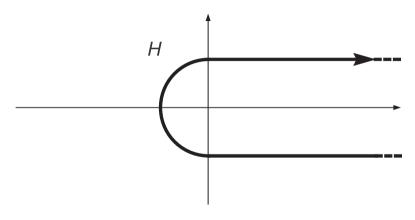
Figure 4: Hankel contour of integration

By using the substitution $y(x)=g(x_{0})-h(x_{0})X+O(X^{2})$ and the relations $w_{0}g(x_{0})=1$, we have

$$1-y(x)w=g(x_{0})(w_{0}-w)+h(x_{0})w_{0}X+O(X^{2}).$$

Hence, if $n$ is large enough we definitely have $1-y(x)w\neq 0$, in particular the term $h(x_{0})w_{0}X+O(X^{2})$ is of minor order of magnitude on these parts of the integration. Consequently we can rewrite the reciprocal of $1-y(x)w$ as

$$\frac{1}{1-y(x)w} =\frac{1}{g(x_{0})(w_{0}-w)+h(x_{0})w_{0}X+O(X^{2})}$$

$$=\frac{1}{g(x_{0})(w_{0}-w)}\left(1-\frac{h(x_{0})w_{0}X}{g(x_{0})(w_{0}-w)}+O\left(\frac{|X|^{2}}{|w_{0}-w|^{2}}\right)\right)$$

$$=\frac{1}{1-\frac{w}{w_{0}}}-\frac{h(x_{0})w_{0}X}{\left(1-\frac{w}{w_{0}}\right)^{2}}+O\left(\frac{|X|^{2}}{|w-w_{0}|^{3}}\right).$$

Next we set $x=x_{0}(1-X^{2})$ and rewrite $G(x,X,w)$ locally as

$$G(x,X,w)=G_{0}(w)+G_{1}(w)X+O(X^{2}).$$

Hence, if $x$ and $w$ are in this range then $f(x,w)$ can be represented as

$$f(x,w) =\left(G_{0}(w)+G_{1}(w)X+O(X^{2})\right)\left(\frac{1}{1-\frac{w}{w_{0}}}-\frac{h(x_{0})w_{0}X}{\left(1-\frac{w}{w_{0}}\right)^{2}}+O\left(\frac{|X|^{2}}{|w-w_{0}|^{3}}\right)\right)$$

$$=\frac{G_{0}(w)}{1-\frac{w}{w_{0}}}-\frac{G(x_{0},0,w_{0})h(x_{0})w_{0}X}{\left(1-\frac{w}{w_{0}}\right)^{2}}+O\left(\frac{|X|}{\left|1-\frac{w}{w_{0}}\right|}\right).$$

The first term does not depend on $x$, hence it does not contribute for $n\geq 1$. The second term provides the asymptotic leading term

$$\frac{1}{(2\pi i)^{2}}\int\limits_{\gamma_{1}\cup\gamma_{2}\cup\gamma_{3}}\int\limits_{\Gamma_{1}\cup\Gamma_{2}\cup\Gamma_{3}}\frac{G(x_{0},0,w_{0})h(x_{0})w_{0}X}{\left(1-\frac{w}{w_{0}}\right)^{2}}\,x^{-n-1}w^{-k-1}\,dx\,dw$$

$$\qquad=-\frac{G(x_{0},0,w_{0})h(x_{0})}{2\sqrt{\pi}}\,g(x_{0})^{k-1}x_{0}^{-n}k\,n^{-\frac{3}{2}}\left(1+O\left(\frac{1}{k}\right)\right),$$

compare with the methods of Flajolet and Odlyzko [8]. We just remark that $x^{-n}$ and $w^{-k}$ are replaced by

$$x^{-n}=x_{0}^{-n}e^{-t+O(t^{2}/n)}\quad\mbox{and}\quad w^{-k}=w_{0}^{-k}e^{-s+O(s^{2}/k)},$$

so that one can use Hankel’s representation of $1/\Gamma(s)$ to evaluate the resulting integrals asymptotically.

Finally, the remainder term provides an error term of the form

$$\int\limits_{\gamma_{1}\cup\gamma_{2}\cup\gamma_{3}}\int\limits_{\Gamma_{1}\cup\Gamma_{2}\cup\Gamma_{3}}O\left(\frac{|X|}{\left|1-\frac{w}{w_{0}}\right|}\right)|x|^{-n-1}|w|^{-k-1}\,|dx|\,|dw|=O\left(w_{0}^{-k}x_{0}^{-n}n^{-\frac{3}{2}}\right),$$

compare again with [8].

If $x\in\gamma_{1}\cup\gamma_{2}\cup\gamma_{3}$ and $w\in\Gamma_{4}$ we can argue in a similar way. We use the expansions

$$\frac{1}{1-y(x)w} =\frac{1}{1-\frac{w}{w_{0}}}+O\left(\frac{|X|}{\left|1-\frac{w}{w_{0}}\right|^{2}}\right),$$ (5.27)

$$G(x,X,w) =G_{0}(w)+O(|X|),$$ (5.28)

and the bounds $x^{-n}=O(x_{0}^{-n})$ and $w^{-k}=O(w_{0}^{-k}e^{-(\log k)^{2}})$ to observe that

$$\frac{1}{(2\pi i)^{2}}\int\limits_{\gamma_{1}\cup\gamma_{2}\cup\gamma_{3}}\int\limits_{\Gamma_{4}}\left(\frac{G_{0}(w)}{1-\frac{w}{w_{0}}}+O\left(\frac{|X|}{\left|1-\frac{w}{w_{0}}\right|}\right)\right)x^{-n-1}w^{-k-1}\,dx\,dw$$

$$\qquad=O\left(w_{0}^{-k}x_{0}^{-n}ke^{-(\log k)^{2}}n^{-\frac{3}{2}}\right).$$

Note that the first term does not depend on $x$ and does not contribute if $n\geq 1$.

Next suppose that $x\in\gamma_{4}$ and $w\in\Gamma_{1}\cup\Gamma_{2}\cup\Gamma_{3}$. In this case we need not be that precise. We can use the estimates $G(x,X,w)=O(1)$ and $|1-y(x)w|\geq c/k\geq c^{\prime}/\log n$ (for certain positive constants $c,c^{\prime}$). Furthermore we have $x^{-n}=O(x_{0}^{-n}e^{-(\log n)^{2}})$ and $w^{-k}=O(w_{0}^{-k})$. Hence the corresponding integral can be estimated by

$$\frac{1}{(2\pi i)^{2}}\int\limits_{\gamma_{4}}\int\limits_{\Gamma_{1}\cup\Gamma_{2}\cup\Gamma_{3}}\frac{G(x,X,w)}{1-y(x)w}x^{-n-1}w^{-k}\,dx\,dw=O\left(x_{0}^{-n}w_{0}^{-k}\log n\,e^{-(\log n)^{2}})\right),$$

which is negligible compared to the asymptotic leading term.

Finally, if $x\in\gamma_{4}$ and $w\in\Gamma_{4}$, the corresponding integral just provides an error term of the form

$$O\left(x_{0}^{-n}w_{0}^{-k}\log n\,e^{-(\log n)^{2}-(\log k)^{2})}\right),$$

which is again negligible. This proves the asymptotic expansion (3.4).

In order to show the upper bound (3.5) we use again Cauchy’s formula for $x\in\gamma_{1}\cup\gamma_{2}\cup\gamma_{3}\cup\gamma_{4}$ (as above) and $|w|=w_{0}(1-\delta)$ for some $\delta>0$. If $x\in\gamma_{1}\cup\gamma_{2}\cup\gamma_{3}$ we use the expansions (5.27) and (5.28) to obtain

$$\frac{1}{(2\pi i)^{2}}\int\limits_{\gamma_{1}\cup\gamma_{2}\cup\gamma_{3}}\int\limits_{|w|=w_{0}(1-\delta)}\left(\frac{G_{0}(w)}{1-\frac{w}{w_{0}}}+O\left(\frac{|X|}{\left|1-\frac{w}{w_{0}}\right|}\right)\right)x^{-n-1}w^{-k-1}\,dx\,dw$$

$$\qquad=O\left(w_{0}^{-k}(1-\delta)^{-k}x_{0}^{-n}n^{-\frac{3}{2}}\right).$$

The integral over $x\in\gamma_{4}$ and $|w|=w_{0}(1-\delta)$ can be estimated directly (and similarly to the above), which leads to an additional error term of the form

$$O\left(x_{0}^{-n}w_{0}^{-k}(1-\delta)^{-k}e^{-(\log n)^{2}}\right).$$

This completes the proof of (3.5).

Now suppose that $g(x_{0})<1$. Then the generating function of $f_{n}=\sum_{k}f_{n,k}$ is given by

$$\sum_{n\geq 0}f_{n}x^{n}=f(x,1)=\frac{G(x,X,1)}{1-y(x)}.$$

By a local expansion it follows that

$$\frac{G(x,X,1)}{1-y(x)}=\frac{G(x_{0},0,1)}{1-g(x_{0})}-\frac{h(x_{0})G(x_{0},0,1)-(1-g(x_{0}))G_{v}(x_{0},0,1)}{(1-g(x_{0}))^{2}}X+O(X^{2}),$$

which induces an asymptotic expansion for $f_{n}$ of the form

$$f_{n}\sim\frac{h(x_{0})G(x_{0},0,1)-(1-g(x_{0}))G_{v}(x_{0},0,1)}{2\sqrt{\pi}(1-g(x_{0}))^{2}}x_{0}^{-n}n^{-3/2}.$$

Similarly we can derive an asymptotic expansion for

$$\sum_{k}f_{n,k}w^{k}=[x^{n}]f(x,w),$$

which shows that the limit

$$\lim_{n\to\infty}\sum_{k}\frac{f_{n,k}}{f_{n}}w^{k}$$

exists uniformly for $|w|\leq 1$. This also shows the existence of the limits $\overline{d}_{k}=\lim_{n\to\infty}f_{n,k}/f_{n}$. ∎

Proof of Lemma 3.2.

The proof of Lemma 3.2 is very close to that of Lemma 3.1. The essential observation is an asymptotic representation of $f(x,w,t)$ of the form

$$f(x,w,t) =\frac{G(x_{0},0,w_{0},w_{0})}{X\left(1-\frac{w}{w_{0}}\right)^{2}\left(1-\frac{t}{w_{0}}\right)^{2}}-\frac{2h(x_{0})G_{0}(w,t)}{1-\frac{w}{w_{0}}}$$

$$-\frac{2h(x_{0})G_{0}(w,t)}{1-\frac{t}{w_{0}}}+O\left(\frac{X}{|w-w_{0}|}+\frac{X}{|t-w_{0}|}\right),$$

for $(x,w,t)$ close to the singularity $(x_{0},w_{0},w_{0})$, and the fact that the first term is the asymptotic leading one. ∎

Proof of Lemma 3.3.

The main observation is that $f(x,w)$ can be approximated by

$$f(x,w) =G(x_{0},0,w_{0})\,\exp\left(\frac{H(x_{0},0,w)}{1-\frac{w}{w_{0}}}\right)$$

$$\quad\times\Biggl{(}1+\Biggl{(}\frac{G(x_{0},0,w)}{G_{v}(x_{0},0,w)}+\frac{H_{v}(x_{0},0,w)}{1-\frac{w}{w_{0}}}-\frac{H(x_{0},0,w)h(x_{0})w_{0}}{\left(1-\frac{w}{w_{0}}\right)^{2}}\Biggr{)}X$$

$$\qquad\qquad+O\left(\frac{X^{2}}{|w-w_{0}|^{3}}\right)\Biggr{)}$$

if $x$ and $w$ are close to their singularities $x_{0}$ and $w_{0}$. Hence, the term

$$-G(x_{0},0,w_{0})\,\exp\left(\frac{H(x_{0},0,w)}{1-\frac{w}{w_{0}}}\right)\frac{h(x_{0})H(x_{0},0,w_{0})w_{0}X}{\left(1-\frac{w}{w_{0}}\right)^{2}}$$

leads to the asymptotic expansion as claimed. The main difference with the proof of Lemma 3.1 is that the contour integration with respect to $w$ is a circle $|w|=w_{0}(1-\eta)$, where $\eta\sim ck^{-1/2}$ is chosen such that $w_{0}(1-\eta)$ becomes a saddle point of the integrand; compare with Hayman’s method [11] and with [1]. All error terms can be easily estimated. ∎

Proof of Lemma 3.4.

The proof is (more or less) a direct combination of the methods used in the proof of Lemma 3.1 and 3.3. The main observation here is that the asymptotic leading term of $f(x,w,t)$ is of the form

$$\frac{G(x_{0},0,w_{0},w_{0})}{X}\,\frac{\displaystyle\exp\left(\frac{H(x_{0},0,w)}{1-w/{w_{0}}}+\frac{H(x_{0},0,t)}{1-t/{w_{0}}}\right)}{\left(1-w/{w_{0}}\right)^{2}\left(1-t/{w_{0}}\right)^{2}}.$$

∎

Proof of Lemma 5.3.

We can neglect the function $G(x,X,w)$ since it is analytic in $w$ around the critical point $(x_{0},w_{0})$.

The main observation now it that the remaining part can be represented (locally) as

$$H(x,X,w)\left(1-\frac{w}{w_{0}}+h(x_{0})w_{0}X+O(X^{2})\right)^{3/2}$$

$$=H(x,X,w)\left(1-\frac{w}{w_{0}}\right)^{3/2}\left(1+\frac{(3/2)h(x_{0})w_{0}X}{1-\frac{w}{w_{0}}}+O\left(\frac{X^{2}}{|w-w_{0}|}\right)\right).$$

Hence, the main contribution comes from the term

$$\frac{3}{2}h(x_{0})w_{0}H(x_{0},0,w_{0})\left(1-\frac{w}{w_{0}}\right)^{1/2}\left(1-\frac{x}{x_{0}}\right)^{1/2}.$$

∎

Prof of Lemma 5.4.

The proof is an easy combination of the proofs of Lemma 5.3 and 3.2. The asymptotic leading term of $f(x,w,t)$ is given by

$$\frac{G_{4}(x_{0},0,w_{0},w_{0})}{X}\left(1-\frac{w}{w_{0}}\right)^{1/2}\left(1-\frac{t}{w_{0}}\right)^{1/2}.$$

∎

References

- [1] N. Bernasconi, K. Panagiotou, A. Steger, The degree sequence of random graphs from subcritical classes, Combin. Probab. Comput. 18 (2009), 647–681.
- [2] M. Bodirsky, O. Giménez, M. Kang and M. Noy, Enumeration and limit laws for series-parallel graphs. Europ. J. Combin. 8 (2007), 2091–2105.
- [3] M. Drmota, A bivariate asymptotic expansion of coefficients of powers of generating functions, European J. Combin. 15 (1994), no. 2, 139–152
- [4] M. Drmota, Random Trees, Springer, Wien-New York, 2009.
- [5] M. Drmota, O. Giménez, M. Noy, Vertices of given degree in series-parallel graphs, Random Structures Algorithms 36 (2010), 273–314.
- [6] M. Drmota, O. Giménez, M. Noy, Degree distribution in random planar graphs, arXiv:0911.4331
- [7] M. Drmota, O. Giménez, M. and Noy, The maximum degree of planar graphs II, manuscript in preparation.
- [8] P. Flajolet and A. Odlyzko, Singularity analysis of generating functions, SIAM J. Discrete Math. 3 (1990), 216– 240.
- [9] P. Flajolet, R. Sedgewick, Analytic Combinatorics, Cambridge University Press, Cambridge (2009).
- [10] Z. Gao and N. C. Wormald, The distribution of the maximum vertex degree in random planar maps. J. Combin. Theory Ser. A 89 (2000), 201–230.
- [11] W. K. Hayman, A generalisation of Stirling’s formula, J. Reine Angew. Math. 196 (1956), 67–95.
- [12] C. McDiarmid and B. Reed, On the maximum degree of a random planar graph, Combin. Probab. Comput. 17 (2008), 591–601.