The DAFT/FADA survey. I. Photometric redshifts along lines of sight to clusters in the z=[0.4,0.9] interval

Abstract

Context. As a contribution to the understanding of the dark energy concept, the Dark energy American French Team (DAFT, in French FADA) has started a large project to characterize statistically high redshift galaxy clusters, infer cosmological constraints from Weak Lensing Tomography, and understand biases relevant for constraining dark energy and cluster physics in future cluster and cosmological experiments.

Aims. The purpose of this paper is to establish the basis of reference for the photo-$z$ determination used in all our subsequent papers, including weak lensing tomography studies.

Methods. This project is based on a sample of 91 high redshift ($z\geq$0.4), massive ($\mathrel{\mathchoice{\lower 0.5pt\vbox{\halign{$\mathnew\displaystyle\hfil#\hfil$\cr>\crcr\sim\crcr}}}{\lower 0.5pt\vbox{\halign{$\mathnew\textstyle\hfil#\hfil$\cr>\crcr\sim\crcr}}}{\lower 0.5pt\vbox{\halign{$\mathnew\scriptstyle\hfil#\hfil$\cr>\crcr\sim\crcr}}}{\lower 0.5pt\vbox{\halign{$\mathnew\scriptscriptstyle\hfil#\hfil$\cr>\crcr\sim\crcr}}}}3\times 10^{14}$ M_⊙) clusters with existing HST imaging, for which we are presently performing complementary multi-wavelength imaging. This allows us in particular to estimate spectral types and determine accurate photometric redshifts for galaxies along the lines of sight to the first ten clusters for which all the required data are available down to a limit of ${\rm I_{AB}}=24./24.5$ with the LePhare software. The accuracy in redshift is of the order of 0.05 for the range $0.2\leq z\leq 1.5$.

Results. We verified that the technique applied to obtain photometric redshifts works well by comparing our results to with previous works. In clusters, photo-z accuracy is degraded for bright absolute magnitudes and for the latest and earliest type galaxies. The photo-z accuracy also only slightly varies as a function of the spectral type for field galaxies. As a consequence, we find evidence for an environmental dependence of the photo-z accuracy, interpreted as the standard used Spectral Energy Distributions being not very well suited to cluster galaxies. Finally, we modeled the LCDCS 0504 mass with the strong arcs detected along this line of sight.

1 Introduction

The discovery ten years ago of the acceleration of the expansion of the Universe (Riess et al. 1998) which is typically explained by assuming that most of its energy is in the form of an unknown dark energy (DE), is one of the most puzzling issues of modern cosmology. Efforts have therefore been undertaken, such as the Dark Energy Task Force (Albrecht et al. 2006) or the ESA-ESO working group on fundamental physics (Peacock et al. 2006) to design projects to measure DE and determine its nature. As highlighted by these reports, understanding DE requires big surveys to overcome cosmic variance and shot noise as well as new experiments to control the unknown systematic uncertainties.

In this context, galaxy clusters, together with several other probes, are expected to play a major role (e.g. Nichol 2007). These objects have indeed long held a place of importance in astronomy and cosmology. Zwicky (e.g. 1933) inferred from observations of the Coma cluster that the matter in our universe could be in the form of a dark component (this component was first supposed to be low surface brightness diffuse light). The measurement of the baryon fraction in X-ray clusters (e.g. Lubin et al. 1996, Cruddace et al. 1997), combined with big-bang nucleosynthesis constraints allowed to put an upper limit on the matter density of the Universe. The resulting value was considerably less than the theoretically-favored critical density. Cluster number counts (e.g. Evrard 1989) and cluster correlation functions (e.g. Bahcall & Soneira 1983) have been used to constrain the amplitude of mass fluctuations and strengthen support for the Cold Dark Matter (CDM) structure formation paradigm. Galaxy clusters can also be used to test the redshift-distance relation (e.g. Supernovae as standard candles, Baryon Acoustic Oscillations or Weak Lensing Tomography with clusters, e.g. Hu 1999) or the growth of structures through weak lensing, cluster number counts, or integrated Sachs-Wolfe effect. Clusters are also intrinsically interesting in many aspects, including the influence of environment on galaxy formation and evolution. Building a detailed picture of galaxy and large-scale structure growth (e.g. clusters) is therefore necessary to understand how the Universe has evolved.

The Dark energy American French Team (DAFT, in French FADA) has started a large project to characterize statistically high redshift galaxy clusters, infer cosmological constraints from Weak Lensing Tomography, and understand biases relevant for constraining DE and cluster physics in future cluster and cosmological experiments. This work is based on a sample of 91 high redshift (z=[0.4;0.9]), massive ($>3\times 10^{14}$ M_⊙) clusters with existing HST imaging, for which we are presently performing complementary multi-wavelength imaging. This will allow us in particular to estimate accurate photometric redshifts for as many galaxies as possible. The requested accuracy depends on both our ability to discriminate between cluster and background field galaxies without loosing too many objects and on the Weak Lensing Tomography method internal parameters. Catalogs of cluster galaxies (e.g. Adami et al. 2008) typically show photometric redshifts spanning a total ($\sim 3\sigma$) interval of $\pm$0.15 in photo$-z$. This means that the goal of our survey is to have photometric redshifts with a 1$\sigma$ precision better than 0.05. With such a precision, the photo-$z$ uncertainties would not be the expected dominant source of errors in our method, except when considering lensing and lensed objects at redshift greater than 0.8 and closer than 0.4 along the redshift direction. The immediate goal of this paper is then to describe these photometric redshift measurements on the first 10 completed clusters in our sample. This will allow us in the future to combine photo-$z$s with weak lensing shear measurements both to carry out tomography and to build mass models for clusters. This paper will also provide the foundation for other future works that will use the photo-$z$s produced by the process described here to study cluster galaxy populations.

Throughout the paper we assume H₀ = 71 km s^-1 Mpc^-1, $\Omega_{m}$=0.27, and $\Omega_{\Lambda}$=0.73. All magnitudes are in the $AB$ system.

2 Observations

The 10 clusters for which we produced photometric redshifts (hereafter photo-zs ) were originally observed as part of the EDisCS program (e.g. White et al. 2005), but new data (mostly B, but also R and z^′, see Table 1) were obtained and some data were also collected from the literature (V, R, I, z^′, F814W, Spitzer IRAC) to complete the data set in order to calculate more accurate photo-zs. We thus created a full data set with BVRIz’, HST ACS F814W, and Spitzer IRAC 3.6 $\mu$m and 4.5$\mu$m (channels 1 & 2). Fig. 1 shows the spectral coverage achieved with this set of filters.

Figure 1: Transmission curves of the available sets of filters. Upper figure: infrared filters (Irac 1: cyan, Irac2: blue). Lower figure: visible filters (from left to right: B, V, R, I in green, F814W in yellow, and z^′).

2.1 HST ACS data

We have retrieved from the HST archives data for 10 EDisCS clusters observed with the ACS in the F814W filter, each image including 4 tiles (2$\times$2 mosaic) of 2 ks and a central tile of 8 ks (Desai et al. 2007). The achieved depth for point sources at the 90$\%$ level is of the order of F814W$\sim$28 for the deep parts and F814W$\sim$26 for the shallow parts (see Fig. 4) . The full data reduction technique is described in Schrabback et al. (2010) and will be expanded in a companion paper (Clowe et al. in preparation), but we give here the salient points. The data were reduced using a modified version of the HAGGLeS pipeline, with careful background subtraction, improved bad pixel masking, and proper image registration. Stacking and cosmic ray rejection were done with Multidrizzle (MD) (Koekemoer et al. 2002), taking the time-dependent field-distortion model from Anderson et al. (2007) into account. The pixel scale was 0.05 arcsec and we used a Lanczos3 kernel. After aligning the exposures of each tile separately, shifts and rotations between the tiles were determined from separate stacks by measuring the positions of objects in the overlap regions. As final step, mosaic stacks including all tiles of one cluster were created. We set these ACS mosaics as astrometric references for ground-based data. Our first results based on weak lensing measurements and weak lensing tomography will be described in a companion papers (Clowe et al., in preparation).

2.2 B, R and z^′ ground based data

The new B, R and z’ band observations presented here were conducted at the CTIO Blanco telescope using the multi-CCD device MOSAIC (see Table 1). Exposure times were computed to reach an expected depth of F814W$\sim$24.5 (AB) at the 10$\sigma$ level. The seeing was on average about 1.1 arcsec, 0.7 arcsec and 0.9 arcsec for the B, R and z bands respectively. During the observations, we followed a regular dithering pattern with an amplitude of 5–10 arcsec to improve cosmetics (e.g. inter-chip separations) of the final images. The standard star fields SA98, SA104, SA107a and SA107b were also regularly observed during the nights (3 standard stars per night). This allowed us to derive extinction curves for the Blanco site and perform photometric calibrations.

Table 1: Decimal degrees J2000 coordinates, observed bands, CTIO exposure times, and redshift for each of the ten considered clusters.

cluster name	RA	DEC	band	exposure time	z	90$\%$ completeness level
	deg	deg		seconds		F814W magnitude
LCDCS 0110	159.464	$-12.724$	B	11x600	0.58	26.2
LCDCS 0130	160.168	$-11.934$	B	11x600	0.70	26.2
LCDCS 0172	163.601	$-11.772$	B	11x600	0.70	26.2
LCDCS 0173	163.681	$-12.764$	B	11x600	0.75	26.2
CLJ1103.7-1245a	165.895	$-12.780$	B	11x600	0.63	26.2
LCDCS 0340	174.542	$-11.560$	B	11x600	0.48	26.2
LCDCS 0504	184.189	$-12.022$	B	11x600	0.79	26.2
LCDCS 0531	186.995	$-11.587$	B	11x600	0.64	26.2
LCDCS 0541	188.126	$-12.8434$	z’	18x500	0.54	25.8
			R	8 x 600		26.6
LCDCS 0853	208.541	$-12.517$	B	11x600	0.76	26.2

2.3 Tools

For the image reduction, we used the MIDAS, SCAMP and SWarp (e.g. Bertin et al. 2002, Bertin 2006) packages to produce images with cosmic rays and other image defects removed, and to produce final calibrated and aligned images; these newly acquired data have then been combined with the previously reduced data. Descriptions of the MissFits, SCAMP and SWarp software are given in http://www.astromatic.net. We co-aligned the FITS images in different bands by using SCAMP and then combined them to generate panchromatic images (see e.g. Fig. 3).

2.4 Ground based data reduction

After the classical reduction scheme (offsets, flatfields, etc.), we realized that the gains between the different MOSAIC CCDs were not initially very well constrained. To solve this problem, we observed a SDSS field in all the bands, which allowed us to adjust these gains. These corrections were in most cases smaller than 10%.

The SCAMP and SWarp tools were used to perform the astrometry and homogenize internal photometry in order to put each of the individual images on a common grid to create a merged image without cosmic rays, with inter-chip gaps filled and CCD defaults erased. This is a commonly employed technique for the CFHT Megacam and CFH12K images (e.g. McCracken et al. 2003). We usually found it necessary to use a third-order polynomial to model the astrometric distortions. We then generated weight maps which took into account bad pixels, overscans and low efficiency areas. Fig. 2 shows the resulting astrometric distortion map obtained for one of the B band observations.

Figure 2: Resulting astrometric distortion map for one of our B band observations. Large black rectangles are the individual MOSAIC CCDs. Blue to red colors show 0.25 to 0.27 arcsec astrometry residual uncertainties.

We then used standard stars observed during the nights to build extinction curves.

The CCDs from MOSAIC are affected by some cross talk. We corrected for this effect by subtracting from a contaminated (receiving) CCD the contaminating (sending) CCD weighted by a factor given on the web page of MOSAIC (http://www.lsstmail.org/noao/mosaic/calibs.html). In any case, this only affected bright magnitude objects. However, considering that the number of such objects per CCD was non-negligible, we had to take cross-talk into account.

Figure 3: LCDCS 0541 tricolor image (50 arcsec $\times$ 30 arcsec) made with the B (CTIO: shown as blue), F814 (HST: shown as green) and z^′ (VLT: shown as red) filters. Known spectroscopic redshifts are also shown.

2.5 Completeness level

Although completeness per se is not important for our goal of obtaining photo-$z$s of the background searched galaxies, it is interesting to discuss this issue because net completeness determines how many galaxies we will have in the end to carry out weak lensing tomography and cluster studies. The first important parameter to estimate is the completeness level of our images in each band. Based on this information we can then determine the magnitude range where all our bands can contribute. To estimate this level, we ran simulations for the HST ACS F814W images as in Adami et al. (2006). In brief, the simulation method adds 100 artificial stars of different magnitudes to the CCD images and then attempts to recover them by running SExtractor again with the same parameters used for object detection on the original images. In this way, the completeness is measured on the original images. We investigated the catalog completeness for point-like sources only. The completeness levels in magnitudes are therefore an upper value for the real completeness level for galaxies of different types.

For the other bands, we computed how many objects detected in the HST ACS F814W images also gave a successful magnitude measurement in the other bands when extracted in SExtractor double-image mode (to increase the depth of the catalogs). We note that the HST ACS F814W images are the deepest among all our bands by a large factor. Multiplying these percentages (not always 100$\%$ because objects are sometimes so close to the background in a given band that the fluxes are not significantly positive) by the completeness of the HST ACS F814W images themselves, we therefore estimate the $complete\leavevmode\nobreak\ detection\leavevmode\nobreak\ level$ of the considered band (as function of the F814W magnitude).

This method also has the following consequence: we must take into account the varying exposure times in the HST ACS F814W images (the centers have longer exposure times than the edges). This results in a varying mean signal to noise in the HST ACS F814W images and we had therefore to adapt the extraction and measure SExtractor signal to noise ratios. We therefore estimated the point source completeness separately in the deep (10 ksec) and shallow (2 ksec) portions of the HST ACS F814W images. This also gave two different $complete\leavevmode\nobreak\ detection\leavevmode\nobreak\ levels$ for the other bands.

The results are displayed in Fig. 4 for LCDCS 0541 (other clusters show very similar results). This shows that considering point sources brighter than F814W=24.5 in the HST ACS F814W deep parts ensures that our data are more than 90% complete whatever the considered band. In the HST ACS F814W shallow parts, the same limit ensures that our data are more than 90% complete for the ground based plus HST ACS F814W images, and more than 80% complete for the Spitzer data. F814W=24.5 therefore seems to be a reasonable compromise between depth and completeness level. This value is also close to the expected value given the chosen exposure times. If we accept lower completeness levels of the order of 50% in all the bands, we can consider magnitudes as faint as F814W=26. Since we can carry out shear measurements down to even fainter magnitudes, this completeness result means we will be able to use a sizable fraction of those shear measurements.

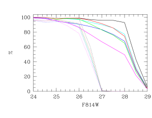
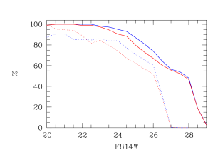
Figure 4: Detection levels for point sources in the LCDCS 0541 fields. Continuous lines correspond to the deep parts of the HST ACS F814W images and dotted lines to the shallow parts. Top figure: blue: B band, cyan: V band, green: R band, red: I band, black: F814W band, magenta: z’ band. Bottom figure: blue: Irac 1 band, red: Irac 2 band. Each curve is given as a function of the F814W magnitude.

$Detection\leavevmode\nobreak\ levels$ are also interresting to compute for future uses for a given band in itself, detecting $and$ measuring the fluxes in this band without considering the HST ACS F814W image as a detection image. We note however that resulting catalogs would then be shallower than previously. We therefore performed the same simulations we did for the HST ACS F814W images for the B, V, R, I, z’, Irac 1, and Irac 2 bands (Sextractor detection level of 1.8, point sources). Fig. 5 gives the corresponding results.

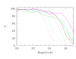
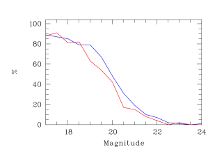
Figure 5: Top figure: detection levels for point sources in the B, V, R, I, z’ bands. Continuous lines correspond to the EDISCS data and dashed lines correspond to the CTIO data. blue: B band, cyan: V band, green: R band, red: I band, magenta: z’ band. Bottom figure: blue: Irac 1 band, red: Irac 2 band.

2.6 Star/galaxy separation

The second step in our processing was to carry out a star-galaxy separation. We only applied this task to the HST ACS F814W images because they have by far the best seeing. For this task we employed the classical method consisting in separating stars from galaxies (and from defects) in central surface brightness versus total magnitude plots. We show in Fig. 6 that the star/galaxy discrimination is efficient up to F814W$\sim$27 (fainter than the initially expected depth for our multi wavelength survey).

Figure 6: Central surface brightness versus total magnitude for the HST ACS F814W LCDCS0541 image. Blue dots are considered as galaxies, red dots as stars, and green dots as defects.

We also had to deal with bright saturated stars. These objects were usually classified as galaxies by classical star/galaxy separation methods. Since we were mainly interested in faint objects, these saturated stars were not really a problem in our analysis. For completeness of our description of our work, however, we investigated what was the contribution of these objects. We examined by eye all F814W$\leq$20 LCDCS 0541 objects and determined a real star catalog. From this, we determined which objects in this list were classified as stars by our automated method based on Fig. 6 and we then deduced the percentage of stars incorrectly classified as galaxies. Fig. 7 gives these percentages as a function of magnitude. We clearly see that limiting our analysis to F814W$\geq$19.5 probably ensures that our galaxy catalogs are not polluted by stars.

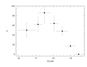
Figure 7: Percentage of saturated stars classified as galaxies by our method as a function of magnitude (see text).

3 Registration with previous images and resulting photo-z computation

We now describe how our new data were combined with the previously acquired data, and how the photo-zs were calculated. We also discuss the reliability of these photo-zs.

3.1 General strategy

In order to calculate photo-zs, the data set had to be combined with data available in the literature. We first re-sampled with SCAMP and SWarp all images to the pixel size of the HST images and the image astrometry was similarly homogenized to produce an alignment precision of the order of one pixel between different bands (1 pixel=0.05 arcsec after realignment).

At this step, the very large CTIO Blanco MOSAIC images ($\sim$30’$\times$30’), the VLT FORS2 images, and the Spitzer IRAC images were truncated to the size of the HST ACS F814W mosaics.

We homogeneously detected and measured objects with the SExtractor package in double image mode (Bertin $\&$ Arnouts 1996). Detection was made on the deepest image (HST ACS F814W image), and measurements were made inside the HST Kron apertures on the ground based B, V, R, I, z^′ images and on the Spitzer Irac 1 and Irac 2 images. At this step, we only kept objects detected in all the available bands.

We could have degraded the HST images to the resolution of the ground based images before extracting sources. However, because we are dealing with clusters of galaxies, this would have resulted in the loss of significant numbers of galaxies in the dense cores. Fig. 8 shows the percentage of recovered objects when degrading the LCDCS 0541 F814W image to a 1 arcsec resolution. We clearly see that $\sim$40 % of the objects are lost at a magnitude of F814W=24.5 and this would strongly penalize our survey.

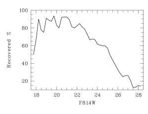
Figure 8: Percentage of recovered objects (detection threshold of 1.8 in SExtractor) in the HST ACS LCDCS 0541 image when degrading the image to a 1 arcsec resolution, as a function of the F814W magnitude.

3.2 Image resolution

Detecting objects in HST images with a spatial resolution sometimes $\sim$10 times better than other images also has non negligible consequences. For example, total magnitudes measured in ground based or in Spitzer images are probably not correct estimates: fluxes computed from $\sim$1 arcsec spatial resolution images inside the HST Kron aperture are obviously underestimates of the total fluxes. However, the main goal of this measure is not to estimate the total magnitude of the objects but to compute photo-zs. The problem can therefore be solved by using the LePhare photo-z package (e.g. Ilbert et al. 2006). Briefly, the LePhare package is able to compare observed magnitudes with predicted ones created by templates from the literature as for example in HyperZ (Bolzonella et al., 2000) or e.g. in Rudnick et al. (2003). We selected spectral energy distributions (hereafter SEDs) from Polletta et al. (2006, 2007) with a Calzetti et al. extinction law (e.g. Calzetti $\&$ Heckman 1999). These are the SEDs which give the best results. The fitting then allows to constrain simultaneously the redshift and nature of each object (galaxy or star), as well as its characteristics such as photometric type (hereafter $T$). With the selected class of SED, $T$ varies from 1 to 31. Numbers between 1 and 7 correspond to elliptical galaxies, numbers between 8 and 12 to S0, Sa, and Sb galaxies (early spiral galaxies), numbers between 13 and 19 to Sc, Sd, and Sdm galaxies (late spiral galaxies), and numbers between 20 and 31 to active galaxies. LePhare is also able to estimate possible shifts in photometric values, by comparing the photometric and spectroscopic redshifts used for training sets, and all the clusters considered in this paper have deep spectroscopic catalogs (see Fig. 10) of $\sim$100 redshifts per line of sight (Halliday et al. 2004 and Milvang-Jensen et al. 2008). Shifts are computed fixing photo-zs to the spectroscopic values and averaging the residuals in each of the bands.

This is useful to take into account internal photometry inhomogeneities between different bands, and also allows us to take into account the different spatial resolutions with LePhare by applying zero point shifts to our magnitudes. The mean (over the ten clusters) applied zero point shifts before photo-z computations in the present paper are $0.00\pm$0.14 (B band), $-0.22\pm 0.06$ (V), $-0.20\pm 0.07$ (R), $-0.18\pm 0.10$ (I), $-0.34\pm 0.08$ (F814W), 0.37$\pm$0.11 (z^′), $-0.86\pm 0.30$ (Irac 1), $-0.92\pm 0.31$ (Irac 2). These values are not negligible, mainly for the Irac 1 and Irac 2 bands. We will now try to estimate the relative contributions to these values of the zero point shifts and of the shifts due to the different spatial resolutions.

A first test to evaluate the influence of the spatial resolution is to compute the shifts to apply in LePhare when degrading the F814W images to a 1 arcsec resolution (close to the resolution of the ground based images). In this case, only the Irac1 and 2 images should require large shifts because they have the worst resolution, of the order of 2 arcsec. The values are equal (for LCDCS 0541) to 0.01 (B band), $-0.14$ (V), $-0.18$ (R), $-0.03$ (I), $-0.15$ (F814W), 0.12 (z^′), $-0.39$ (Irac 1), $-0.44$ (Irac 2). In this case, shifts are rather small and the only large values occur for the two Irac bands, as expected. This means that a large part of the shifts applied to magnitudes in LePhare is probably due to different image resolutions.

We can also evaluate the effect of different resolutions on the images with simulations. We generated artificial objects with FWHM varying from to 0.2 to 1.2 arsec and applied the magnitude measurement process to these images as seen with the HST F814W configuration and as seen in the other bands. Namely, these are B band (seeing of 1.05 arcsec), V (0.68 arcsec), R (0.82 arcsec), I (0.62 arcsec), z’ (0.54 arcsec), and Irac1 and Irac2 (1.9 arcsec). We show in Fig. 9 the differences between true and measured magnitudes as a function of object size for the various filters. These shifts are most of the time lower than 0.2 magnitude, except for the Irac1 and Irac2 bands. At the median object size, Irac1 and Irac2 magnitude shifts are of the order of 0.95, in perfect agreement with the previously quoted shifts estimated with LePhare.

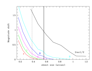
Figure 9: Simulated magnitude shifts to apply in LePhare as a function of object size and for the various bands. The solid vertical line is the median value of the object sizes for F814W$\leq$24.5 in real data. The vertical dashed line shows the minimal size of 90$\%$ of the objects.

3.3 Blended objects

Objects which are nearby ($\sim 1$^′′) but separated in ACS images may be blended in ground based or Spitzer images. Using SExtractor in double image mode avoids the incorrect identification of faint ACS detected objects with incorrect objects in the ground based or Spitzer images. We calculate the flux inside the Kron aperture in the poorer spatial resolution images as determined from the higher spatial resolution image (HST) at the exact place of the faint object. This procedure limits the cross talk between the fluxes. Furthermore, we flag these blends so we can determine if including the objects or not changes the result we derive from our photo-z catalogs in a statistically significant manner. However, as we show below, the quality of the photo-zs for the blends is close to those derived from the non-blended objects.

3.4 Photo-$z$ accuracy with the spectroscopic sample

Given the results of Coupon et al. (2009), our data should be able to provide good photo-zs for magnitudes at least as faint as i^′=24 (AB magnitudes) and for redshifts lower than $\sim$1.5. We first estimate the quality of our photo-zs by comparing them to available spectroscopic redshifts. This gives us insight on the photo-z quality in the magnitude and redshift ranges covered by the spectroscopic catalogs. We show in Fig. 10 the redshift and F814W band magnitude histograms of the available spectroscopic redshifts along the ten considered lines of sight. The photo-z quality assessment will be valid up to z$\sim$1.05 and for magnitudes brighter than $\sim$23.5 and really strong up to z$\sim$1 and for magnitudes brighter than $\sim$23.

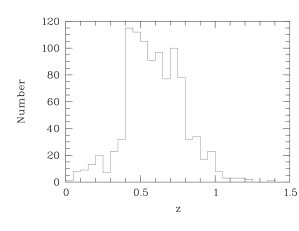
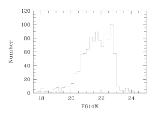
Figure 10: Redshift (top) and F814W magnitude (bottom) histograms of the spectroscopic sample.

We then generated the photo-z versus spectroscopic redshift ($specz$ hereafter) plots shown in Figs. 11 and  12. These plots give the dispersions around the mean relation (both the NMAD reduced sigma of Ilbert et al. (2006) and the regular sigma value: second moment of the value distribution), and the mean shift between photo-zs and $specz$s. We clearly see that on average, photo-zs and $specz$s are in good agreement with a reduced $\sigma$ of the order of 0.05 around the mean relation (regular sigma of the order of 0.09). The percentage of catastrophic errors (objects with a difference between true redshift and photo-z of more than 0.2$\times$(1+$specz$)) is not negligible, but remains lower than 5$\%$. It is also tempting to see an increased uncertainty in the photo-z estimates when considering cluster galaxies (except for LCDCS 0173). We will however quantify this possible effect later in the paper. We also remark that catastrophic errors mainly occur towards the high photometric redshifts (at z$\geq$1.5) and we will discuss the possible consequences on our survey in the final section.

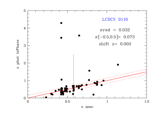
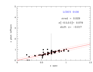
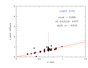
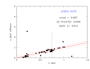
Figure 11: Spectroscopic versus photometric redshifts for 4 clusters. We also give the dispersions around the mean relation (reduced value, classical value excluding galaxies for which the difference between spectroscopic and photometric redshifts is greater than 0.5), and the mean shift between photo-zs and $specz$s. The solid inclined lines give the perfect relation while the dotted lines give the $\pm$0.15 relations. The vertical lines give the position of the cluster along the line of sight.

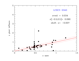
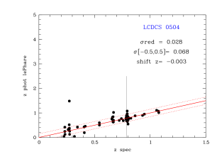
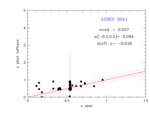
Figure 12: Same as Fig. 11 for the 6 other clusters.

The question is now to know if photo-zs of blended objects are also acceptable. We therefore flagged all such objects by selecting galaxies with a close neighbor (at less than 1.5 arcsec, given the ground based seeings) and less than 0.5 magnitude fainter than the primary object (enough to potentially bias the magnitude estimate). Such objects are potentially polluted by a comparable or brighter object (less than 0.5 magnitude fainter, or brighter). We then generated Fig. 13 where all such objects from the ten considered clusters are shown. The reduced $\sigma$ is 0.08. The percentage of catastrophic errors is $\sim$10%, higher than for the whole sample of galaxies (blended or not). However even if these two values (the reduced $\sigma$ and the percentage of catastrophic errors) are higher than for the whole sample, they remain acceptable for our purposes and we conclude that blending is not a redhibitory problem for z$\leq$1.05 and F814W$\leq$23.5.

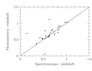
Figure 13: Photometric versus spectroscopic redshifts for the blended objects in the spectroscopic sample.

3.5 Photo-$z$ accuracy and environmental dependence

Although the first goal for the FADA/DAFT project is to determine the photo-zs of background field galaxies, it is also of interest to determine the achieved photo-z accuracy and the fraction of catastrophic errors as a function of various cluster/galaxy internal parameters. In clusters, Adami et al. (2010) have already shown with the X-ray selected XMM-LSS sample that late type galaxies tend to exhibit poorer photo-z precision than early type galaxies. Moreover, the XMM-LSS clusters are not very massive structures and environmental effects are perhaps not as strong as in the presently considered clusters.

With the sample presently in hand, we determined the effect of galaxy type and magnitude on the photo-z accuracy in the redshift range for which spectroscopic data exist. Similarly, we can investigate the possible effects of the environment (cluster versus field regions).

We chose to merge the 10 clusters in a single photometric versus spectroscopic redshift catalog. The following results will therefore apply for the considered cluster redshift range (z [0.4;0.9]). We show in Figs. 14 and  15 the variation of the reduced $\sigma$ of the photo-zs as a function of photometric type and of absolute magnitude for cluster galaxies within a projected cluster-centric radius of 0.5 Mpc and 1 Mpc, and field galaxies. Galaxies were selected as members of the 1 Mpc radius region if their redshift differed by less than 3 times the velocity dispersion of Clowe et al. (2006) compared to the mean cluster redshift. For the 0.5 Mpc region, the limit was set to less than one time the velocity dispersion of Clowe et al. (2006).

These figures show that we have a worse photo-z accuracy for the brightest cluster galaxies (in absolute magnitude). Differences between best and worst values represent most of the time a factor of two, in good agreement with the results of Adami et al. (2010). The tendency is clearly different in the field where the variation is not significant. Considering now the photometric type $T$, we see in Fig. 14 the worse photo-z accuracy for the latest and earliest type objects in cluster regions while again field galaxies do not show any significant tendency.

Considering now catastrophic error percentages, in clusters such errors occur for both bright and late type galaxies. Table 2 gives the spectral type and magnitude intervals for which we have non null catastrophic error percentages in clusters. In the field, these percentages are non null whatever the galaxy type or magnitude and there is no clear trend to have preferably high or low catastrophic error percentages for specific galaxy types or magnitudes.

Table 2: Spectral type and magnitude intervals for a given cluster area for which the percentage of catastrophic errors (4th column) is non null.

Spectral type	Magnitude	Radius	Percentage
$19\leq T\leq 31$	M${}_{i^{\prime}}=[-23,-22]$	1Mpc	11$\pm$11$\%$
$19\leq T\leq 31$	M${}_{i^{\prime}}=[-25,-23]$	1Mpc	28$\pm$19$\%$
$19\leq T\leq 31$	M${}_{i^{\prime}}=[-22,-21]$	0.5Mpc	5$\pm$4$\%$
$19\leq T\leq 31$	M${}_{i^{\prime}}=[-25,-22]$	0.5Mpc	19$\pm$7$\%$
$12\leq$$T$$\leq 19$	M${}_{i^{\prime}}=[-23,-22]$	0.5Mpc	5$\pm$5$\%$

How can these tendencies be understood? It is tempting to say that photometric redshift SEDs are environment dependent. This would not be surprising as the commonly used SEDs are adapted to low density environments and resulting photo-z accuracy could be degraded when considering cluster galaxies. The spectral types showing in clusters the most atypical evolution compared to field objects are early type galaxies (cluster dominant galaxies) and very late type galaxies (galaxies with short bursts of star formation induced by the intracluster influence). These are exactly the ones showing the worst photo-z accuracies in the previous tests. Moreover, during the process of the zero point shift estimates, we recall that we are comparing the photometric and spectroscopic redshifts used for training sets. These training sets are dominated by field galaxies for most of the presently considered lines of sight ($\sim$60$\%$ of the available redshifts are field objects), so photometric redshifts for cluster galaxies may well not be optimally computed. In order to test these possibilities, we computed the shifts to apply to our photometry when including in spectroscopic training sets all the available redshifts or only those belonging to clusters. Fig. 16 shows the difference between these shifts as a function of the considered photometric band disregarding the cluster redshift. Fig. 17 shows the same shifts but at the rest frame wavelength (only for optical bands). This last figure is sensitive to the general SED shape. We clearly see that most of the optical magnitudes need to be brighter to reach the best SED when using cluster training sets, except for the B band which needs to be fainter. From Fig. 17, we can also say that SEDs for cluster galaxies would need to be (sligthly) fainter at red wavelengths and brighter by $\sim$0.1 magnitude at blue wavelengths. The effect remains modest (less than 0.1 magnitude most of the time) but it is nearly systematic over the 10 considered lines of sight. The magnitude shifts computed with the global training sets are therefore not perfectly adapted to cluster galaxies, and used SEDs are also not very well adapted to cluster galaxies. This probably explains part of the photo-z accuracy dependence on the environment. These results therefore confirm the need for high density environment SEDs when high precision photo-zs are required for cluster studies. The main improvement should essentially come from new SEDs for bright and very early or very late type cluster galaxies at various redshifts.

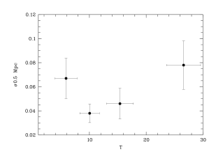
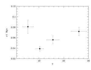
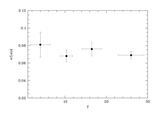
Figure 14: Reduced $\sigma$ of photo-zs versus galaxy photometric type $T$. From top to bottom: cluster galaxies inside a 500 kpc radius, inside a 1 Mpc radius, and field galaxies. Error bars for the types are simply the second order momentum of the galaxy type distribution in the selected type bins ([1;7], [8;12], [13;19], [20;31]). Error bars for the reduced $\sigma$ are Poissonian error bars and are therefore directly proportional to the inverse of the number of galaxies inside the considered bin.

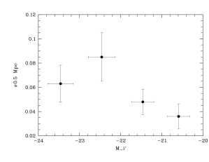
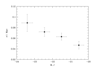
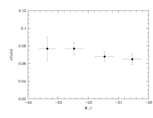
Figure 15: Reduced $\sigma$ of photo-zs versus galaxy i’ absolute magnitude. From top to bottom: cluster galaxies inside a 500 kpc radius, inside a 1 Mpc radius, and field galaxies. Error bars for the absolute magnitudes are simply the second order momentum of the galaxy magnitude distribution in the selected magnitude bins ($[-24;-23],[-23;-22],[-22;-21],[-21;-20]$). Error bars for the reduced $\sigma$ are Poissonian error bars and are therefore directly proportional to the inverse of the number of galaxies inside the considered bin.

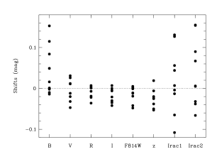
Figure 16: Difference between LePhare estimated magnitude shifts (the value when considering only cluster galaxy redshifts minus the value when considering all available galaxy redshifts) for the various photometric bands considered. A positive value means that magnitudes have to be more weakened when considering cluster galaxy redshifts than when considering all available redshifts (from cluster or field galaxies).

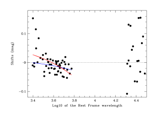
Figure 17: Same as Fig. 16 at the rest frame wavelength. The red inclined line is the regression line for the visible bands. The blue inclined line is the regression line for the visible bands when considering only the shifts smaller than 0.04.

3.6 Photo-$z$ quality checks: beyond the spectroscopic sample limits

We now ask the question of the photo-z quality beyond z=1.05 as well as for objects fainter than F814W=23.5. These ranges cannot be tested with the spectroscopic data in hand, so we chose the same approach as in Ilbert et al. (2009). This paper shows that the percentage of galaxies with an individual photo-z error (estimated by LePhare) larger than a given value is an indicator of the catastrophic error percentages while the mean value of the individual photo-z errors (for a given object subsample) is a good approximation of the dispersion of the $specz$/photo-z relation (for the same subsample).

Before directly applying this approach, we first need to test it on our data. For this, we select galaxies with a spectroscopic redshift and we compute how many times the spectroscopic value falls inside the 1$\sigma$ interval given by the photo-zs. The result is 67$\pm$8%, in good agreement with the expected 68% for the 1$\sigma$ interval. We can therefore quantify the global photo-z accuracy based on the 1$\sigma$ error bars of individual photo-zs.

We then computed the percentage of galaxies with a $1\sigma$ error bar less than $0.2(1+z)$ (similarly as in Adami et al. 2008). This gives us an estimate of the percentage of galaxies with photo-zs which are not catastrophic errors as a function of magnitude and as a function of redshift, even beyond the spectroscopic limit. We plot in Fig. 18 these percentages for the ten merged lines of sight considered. We first confirm that F814W$\leq$23.5 and z$\leq$1.05 galaxies probably have reliable photo-zs, as suggested in the previous section. Moreover, percentages statistically remain globally higher than 90$\%$ for magnitudes brighter than F814W$\sim$24 or 24.5 except in the $z=[1.5;2.0]$ redshift range. As expected, the worse situation appears for the $z=[1.5,2.0]$ range (see also Coupon et al. 2009). The presently available magnitude passbands are not well adapted to this range, the Balmer break being located redward of the z^′ band, and the Lyman break still being bluer than the B band. Finally, galaxy fluxes contaminated by brighter close (blended) neighbors do not seem to show values significantly different from isolated objects. Taken at face value, these results suggest that our photo-zs are not strongly polluted by catastrophic errors down to F814W$\sim$24.5.

We plot in Fig. 19 the mean individual photo-z errors per bin of magnitude as a function of magnitude and photo-z for various redshift intervals. This gives us an estimate of the 1$\sigma$ uncertainty around the $specz$/photo-z relation in the considered redshift interval. We confirm and extend the results of the previous section. Galaxies brighter than F814W$\sim$24.5 and in the z=[0.4;1.5] or brighter than F814W$\sim$24 and in the z=[3.0;6.0] range have relatively low photo-z uncertainties. We also confirm that photo-zs in the z=[1.5;3.75] range are poorly constrained.

These tests therefore lead us to adopt a conservative approach, and to limit our catalogs to galaxies brighter than F814W=24.5 and z$\leq$1.5. We may also consider galaxies brighter than F814W=24 and at z$\geq$3.75.

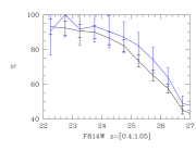
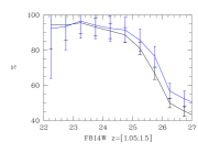
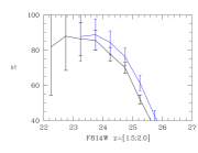
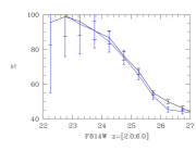
Figure 18: Percentages of galaxies with a photo-z error lower than 0.2*(1+z) as function of magnitude in four redshift bins. Black line: whole sample, blue line: galaxies polluted by a comparably bright or brighter galaxy. We computed the percentages only in the magnitude bins with more than 5 galaxies.

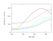
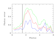
Figure 19: Left: mean individual photo-z uncertainties (regular estimator) as a function of F814W magnitude in four redshift intervals, color coded as: blue: z=[0.4;1.05], green: z=[1.05;1.5], red: z=[1.5;2.0], black: z=[2.0;3.0], cyan: z=[3.0;6.0]. Right: mean individual photo-z uncertainties as a function of photo-z for various F814W magnitude intervals, color coded as: blue: F814W=[19.5;22.5], red: F814W=[19.5;24.5], green: F814W=[19.5;26.]. The vertical line shows the z$\leq$1.5 limit we suggest to adopt in order to use the photo-zs of this paper.

3.7 Photo-$z$ quality checks: the z$\geq$3 domain

As an additional external test of the photo-z uncertainties for distant and faint galaxies, we took advantage of the giant arcs detected along the LCDCS 0504 cluster (see Fig. 20). These arcs are likely to be multiple images of a low number of sources and should therefore have identical redshifts when they originate from a single object. We computed photo-zs for these arcs and at least four of them produced values close in redshift with similar spectral types (T in [21,31], all consistent with an active galaxy). These arcs have F814W magnitudes (measured in the rectangles shown in Fig. 20) of $26.3\pm 0.2$, $23.9\pm 0.1$, $25.5\pm 0.1$ and $24.8\pm 0.1$. We assumed that these four objects were multiple images of a single z$\sim$3.68 galaxy, although we may have two couples of arcs coming from two distinct objects at z$\sim$3.74 and z$\sim$3.62. This allowed us to estimate an upper value of the photo-z uncertainty in this redshift range and at these magnitudes. We found a value of 0.07 even better than the statistical estimates of Fig. 19.

Figure 20: LCDCS 0504 F814W image showing the giant arcs for which we computed photometric redshifts.

As a by product, we also performed a dynamical analysis of LCDCS 0504 from the giant detected arcs (see Appendix A).

3.8 Photo-$z$ quality and spatial resolution

We will now test if systematic effects appear as a function of image resolution. For this, we degraded the HST image of LCDCS0541 to a 1 arcsec resolution. As stressed above, this would lead to an important loss of objects, so we concentrate here only on the photo-z estimate. We repeat all the process of photo-z computation (detection of objects in the HST ACS F814W images, and measurements in the other bands) and correlate the present photo-z estimates with the values coming from the image with no degradation. We show in Fig. 21 the differences between the two estimates, as a function of magnitude. This figure provides evidence for a redshift underestimate for F814W magnitudes fainter than 24. This underestimate is lower than $\sim$0.2 down to F814W=24.5, which remains modest compared to the mean photo-z values also shown in Fig. 21. We therefore conclude that the fact that the spatial resolutions of the considered images differ is not a problem for photo-zs down to F814W$\sim$24.5. This conclusion is in good agreement with the previous sections, where we also proposed to limit the use of photo-zs to objects brighter than F814W$\sim$24.5 (which corresponds to a mean redshift of 1.5, also in good agreement with previous expectations).

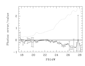
Figure 21: Continuous line (with error bars): photo-z difference for LCDCS 0851 between degraded HST image and full HST resolution, as a function of magnitude. Dotted line: mean photo-z values as a function of magnitude (full HST resolution).

3.9 Do we need Spitzer images to estimate photo-$z$s?

The images with the worse spatial resolution in our sample are the two Irac bands so we need to check if there is any benefit in using these two bands, in particular for objects with F814W$\leq$23.5. We therefore merged spectroscopic redshift catalogs for the ten lines of sight considered and produced a $specz$ versus photo-z diagram with and without Spitzer data (see Fig. 22). The reduced sigma around the mean relation is better when Spitzer data are not considered (0.028 versus 0.031). However, the inclusion of these infrared data reduces by a factor of 3 to 4 the catastrophic error percentage (2$\%$ versus 7$\%$) as computed by Ilbert et al. (2006). This catastrophic error percentage of 2$\%$ is comparable to that found by Coupon et al. (2009). It seems therefore reasonable to pay the price of a slightly higher reduced sigma (but still acceptable and comparable to classical literature values of 0.03 for LePhare, e.g. Coupon et al. 2009) to obtain a catastrophic error percentage lower by a great factor.

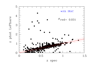
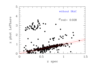
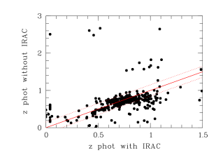
Figure 22: Spectroscopic versus photometric redshifts for the ten lines of sight. Top figure: photo-zs computed with all available bands. Central figure: photo-zs computed without Spitzer data. Bottom figure: photo-zs computed with and without Spitzer data.

4 Comparison with the literature

4.1 General redshift histogram

Now that we have defined a well controlled sample, we compare in this section the resulting photo-z histogram (from the ten merged lines of sight) with known literature redshift distributions. We chose the VVDS deep and ultra deep (LeFèvre et al. 2005, LeFèvre et al. in preparation) surveys because they provide a much more robust spectroscopic redshift distribution than any other literature photo-z distribution. The VVDS deep survey gathers 7266 reliable spectroscopic redshifts down to I_AB$\sim$24.1 over a $\geq$0.6 deg² area. The VVDS ultra deep survey gathers 550 reliable spectroscopic redshifts down to i’_AB$\sim$24.75 over a more limited area of $\sim$400 arcmin². This magnitude limit is very close to F814W=24.5 (an Sc galaxy at z=1.2 has i’$-$F814W$\sim$0.3) and will allow a direct comparison without magnitude limitations.

We re-normalized the two histograms (from the VVDS surveys and from our photo-z catalogs) to the same number of galaxies in order to take into account the different spatial coverages. We then produced Fig. 23 where we can see the generally good agreement between the two distributions. Some differences are visible but are nearly all explained by known clusters along the different lines of sight. The only puzzling differences occur at z$\geq$1.2. They can be explained by the fact that this redshift interval is mainly dominated by VVDS ultra-deep data, which only cover a relatively small area of the sky and are subject to a strong cosmic variance. A second explanation can also be that photo-zs begin to have a decreasing precision beyond z$\sim$1.3 and F814W$\geq$22.5, as shown in Fig. 19.

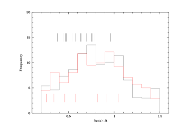
Figure 23: Normalized redshift distributions of our photo-zs (black histogram) superimposed on the VVDS deep and ultra deep spectroscopic redshift distribution (red histogram). Short black vertical lines show the redshift distribution of known NED clusters along our lines of sight. Short red vertical lines show the redshift distribution of known clusters in the VVDS deep survey from Mazure et al. (2007).

4.2 Comparison with EDisCS photo-$z$s

Although Pelló et al. (2009) already computed photo-zs for the EDisCS galaxy cluster sample, there are fundamental differences in the present approach based largely on the difference in goals.

First, we did not use the same photometric bands, due to differing scientific goals. Most of the photo-zs of Pelló et al. (2009) were computed with V, R, I, J, and Ks magnitudes (except for Cl1232-1250 where B, V, I, J, and Ks were selected) because the study was mainly focused on z$\sim$[0.4, 0.8] cluster galaxy populations. All photo-zs in the present study were computed with B, V, R, I, F814W, Spitzer IRAC 3.6 $\mu$m, and 4.5$\mu$m (J and Ks data were not all publicly available at the beginning of the study) because we are also interested in detecting foreground z$\leq$0.4 galaxy populations (to avoid potential pollution of distant galaxy samples) and very high redshift objects. This should lead us to have a better precision at redshifts lower than 0.4 (where the 4000 Å break is not yet bracketed if the B band is not used) and for very distant objects (z$\geq$5). Conversely, our precision will be degraded at z$\geq$1.5, where we lose the 4000 Å break due to our lack of near infrared data. The two approaches are therefore complementary.

Second, Pelló et al. used the 80’s and 90’s Coleman et al. (1980), Bruzual $\&$ Charlot (1993), and Kinney et al. (1996) SEDs. We considered the more recent Polletta et al. (2007) SEDs. These recent templates are becoming standard SEDs because they were optimized for near infrared and infrared data and are therefore well adapted to our set of magnitudes. They were also selected for the COSMOS survey (e.g. Ilbert et al. 2009).

For these two reasons, it is interesting to make a comparison between the two photo-z computations in the common redshift range z$\sim$[0.4, 1.5]. In this range, we compared our reliable photo-zs (galaxies brighter than F814W=24.5, and with 1$\sigma$ uncertainty lower than 0.2$\times$(1+z)) with the HyperZ values of Pelló et al. (2009). Fig. 24 shows a reasonable agreement. This figure exhibits a few objects with large differences between the two estimates. They are all at z$\geq$2 in the HyperZ computations, in good agreement with the fact that Pelló et al. (2009) photo-zs were computed with Ks data. However they represent only 6$\%$ of our total sample and are basically all fainter than F814W=22.5. This percentage is also similar to the previously estimated percentages of catastrophic errors in our estimates. The offset between the two photo-z estimates is $-0.03\pm 0.20$ (1$\sigma$ error bar). This uncertainty of 0.20 has to be compared to the quadratic sum of the LePhare and HyperZ respective uncertainties.

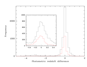
Figure 24: Histogram of the differences between the presently computed reliable photo-zs (galaxies in 19.5$\leq$F814W$\leq$24.5, at redshift lower than 1.5, and with 1$\sigma$ LePhare uncertainty estimate lower than 0.2$\times$(1+z)) and the HyperZ photo-zs of Pelló et al. (2009). The black histogram is for F814W$\leq$24.5 and the red histogram is for F814W$\leq$22.5. The inner figure is a magnification of the central peak.

These comparisons therefore validate our current approach.

5 Summary

We computed photo-zs with the LePhare package for ten relatively distant cluster lines of sight selecting B, V, R, I, F814W, z’, Spitzer IRAC 3.6 $\mu$m, and 4.5$\mu$m images. These images were reduced and aligned at the pixel scale using the SCAMP and SWarp tools. The zero points of the various bands were adjusted by LePhare using publicly available spectroscopy.

The photo-zs prove to be reliable in the z$\sim$[0.4, 1.5] redshift range and in the magnitude range F814W$\sim$[19.5, 24.5]. They are also relatively reliable in the z$\sim$[3.75, 6.0] redshift range and in the magnitude range F814W$\sim$[19.5, 24.]. We remarked that catastrophic errors mainly occured towards the high photometric redshifts (at z$\geq$1.5). This will obviously not affect our survey when limiting our analysis to the [0.4, 1.5] redshift range. The only consequence would be to remove a small number of galaxies. If we also consider the z$\sim$[3.75, 6.0] redshift range, we will include in our future weak lensing analyses some galaxies (of the order of 2$\%$ from the spectroscopic redshift sample estimate) with completely wrong redshifts. Given the limited amount of such galaxies, the consequences on our survey will however remain limited. We achieved a photo-z precision of the order of 0.05 for the full sample. This precision is degraded by a factor of two when considering blended objects.

The photo-z catalogs produced will therefore allow future weak lensing tomography measurements as well as mass modeling of the 10 clusters presently considered. We already used strong lensing features in order to model the mass of LCDCS 0504 (see Appendix A).

We also present evidence for environmental dependence of the photo-z precision. We show that in dense regions (cluster centers or peripheral cluster areas), photo-z precision for bright galaxies is of the order of 0.07 while it is of the order of 0.04 for faint galaxies. We detect the same variation in clusters when considering galaxies as a function of their spectral type. The photo-zs are better estimated for S0 galaxies ($\sim$0.04) than for late type galaxies by a factor of about 2. Considering now galaxies in the sample not related to clusters, the photo-z precision only slightly varies as a function of galaxy spectral type and absolute magnitude. We reach similar conclusions in Adami et al. (2010) based on Coleman et al. (1980) SEDs instead of the Polletta et al. (2007) SEDs. The catastrophic error percentages give similar results. The largest catastrophic error percentages occur in clusters for bright and late type galaxies. In the field, we have similar percentages whatever the galaxy magnitudes and spectral types. This leads us to conclude that regular field-based SEDs available in the literature are not very well adapted to high density environments. The agreement between spectroscopic and photometric redshifts stays acceptable most of the time, but could penalize cluster studies when a precise cluster membership is required. In this framework, we therefore plan in a future work to build such high-density region SEDs with long based spectral range instruments as VLT/X-Shooter, in order to have SEDs usable for cluster galaxies. The VLT/X-Shooter spectral coverage of $\sim$[300,2500]nm for z$\sim$0 galaxies should for example be able to provide a large enough interval to constrain B to Irac1 bands at z$\sim$0.4 and V to Irac2 bands at z$\sim$0.9. We also plan to observe more distant objects than z$\sim$0 galaxies in order to limit possible evolutionary effects. The most important galaxies to target are bright objects (M${}_{i^{\prime}}\leq-23$) making these targets easy to observe. The VLT/X-Shooter should for example be able to provide signal to noise better than 5 over the available spectral range in a 2 hours integration for a z=0.1 elliptical galaxy and better than 5 redder than 4000 A in a 4 hours integration for a z=0.4 elliptical galaxy.

As external tests, we also compared the redshift histogram of our photo-zs with the redshift histogram from a spectroscopic survey, the VVDS, and we find a good agreement. We also directly compared our photo-zs with the estimates of Pelló et al. (2009), and we also have a good agreement in the redshift range where both computations are reliable.

Finally, we stress that the data we present here are part of a larger survey, the DAFT/FADA survey. The present paper will therefore act as a reference study for all subsequent articles. An important aspect is that our data will be made available to the astronomical community at the end of the survey, via a dedicated structure included in the Marseille CENCOS data center (http://cencosw.oamp.fr/).

Appendix A The Einstein Radius of LCDCS 0504

LCDCS 0504 has prominent arc features (see Fig. 20) that form a near circular ring. We can use these arcs to make a simple estimate of the mass inside the ring by assuming circular symmetry. A completely circular mass model results in a complete Einstein ring. We calculate the Einstein radius for the three knots in this arc (seen on both sides of the cluster: a, b, c, see Fig. 25) and find $\theta_{E}=16.28\pm 0.02$ arcseconds.

Figure 25: LCDCS 0504 trichromic image showing the arcs selected to estimate the Einstein radius.

The Einstein radius for a circular mass distribution is defined by the equation:

$$\theta_{E}=\sqrt{\frac{4G\leavevmode\nobreak\ m(\theta_{E})}{c^{2}}\leavevmode\nobreak\ \frac{d_{LS}}{d_{L}d_{S}}}$$ (1)

where $m(\theta)$ is the projected or cylindrical mass inside an angle $\theta$ and $d_{L}$, $d_{S}$ and $d_{LS}$ are the usual angular diameter distances, to the lens, to the source and between the lens and the source respectively. It is easily shown that this equation is equivalent to the equation $\gamma(\theta_{E})+\kappa(\theta_{E})$=1 where $\gamma$ and $\kappa$ are the shear and convergence.

For an isothermal sphere, with velocity dispersion $\sigma$, $\gamma(\theta)=\kappa(\theta)=2\pi(\sigma/c)^{2}(d_{LS}/d_{S})\leavevmode\nobreak\ \theta^{-1}$ and so $\theta_{E}=4\pi(\sigma/c)^{2}(d_{LS}/d_{S})$.

We have measured the photometric redshifts of the faint blue arcs and determined $z_{S}=3.7$. The redshift of the lens is $z_{L}=0.7943$ (Halliday et al. 2004). This allows us to calculate the angular diameter distances and to determine the velocity dispersion of the isothermal model. We find, $\sigma=969\pm 50$ km/s with the 5% error dominated by the model dependence and the assumption of circular symmetry. This is in good agreement with $\sigma=1018\pm 75$ km/s, the velocity dispersion measured by Halliday et al. (2004).

Another model to consider would be the NFW model. The Einstein radius can be calculated numerically from the condition $\gamma(\theta_{E})+\kappa(\theta_{E})$=1 using the well known formulae (e.g. Wright & Brainerd 2000) for the NFW profile. The NFW model has two parameters $r_{200}$ and $c_{200}$. With the one constraint from $\theta_{E}$, there is a degeneracy between these two parameters and so $r_{200}$ depends on the assumption on $c_{200}$ and vice versa. We give the resultant $r_{200}$ and $M_{200}$ (the 3D mass inside $r_{200}$) for various $c_{200}$ in Table 3.

Table 3: $r_{200}$ and $M_{200}$ (the 3D mass inside $r_{200}$) for various $c_{200}$.

$c_{200}$	$R_{200}\leavevmode\nobreak\ (h^{-1}$ Mpc)	$M_{200}\leavevmode\nobreak\ (h^{-1}M_{\odot})$
3	1.19	9.00 $\times 10^{14}$
5	0.98	5.62 $\times 10^{14}$
7	0.87	3.96 $\times 10^{14}$
10	0.79	2.61 $\times 10^{14}$

In general the relation between $c_{200}$ and $r_{200}$, consistent with our constraint, is given by the following fitting function:

$ln(r_{200})=\sum_{i}p_{i}\ln(c_{200})^{i}$ with $p_{0}=0.58485295,p_{1}=-0.29387216,p_{2}=-0.12836863,p_{3}=0.057980625$ and $p_{4}=-0.0061749105$.