Observational constraints on the energy scale of inflation
Abstract
Determining the energy scale of inflation is crucial to understand the nature of inflation in the early Universe. Assuming a power-law power spectrum of primordial curvature perturbations, we place observational constraints on the energy scale of the observable part of the inflaton potential by combining the 7-year Wilkinson Microwave Anisotropy Probe data with distance measurements from the baryon acoustic oscillations in the distribution of galaxies and the Hubble constant measurement. Our analysis provides an upper limit on this energy scale, GeV at 95% confidence level. Moreover, we forecast the sensitivity and constraints achievable by the Planck experiment by performing Monte Carlo studies on simulated data. Planck could significantly improve the constraints on the energy scale of inflation and on the shape of the inflaton potential.
pacs:
98.80.CqI Introduction
Inflation in the early Universe has become the standard model for the generation of cosmological perturbations in the Universe, the seeds for large-scale structure and temperature anisotropies of the Cosmic Microwave Background (CMB). The simplest scenario of cosmological inflation is based upon a single, minimally coupled scalar field with a flat potential. Quantum fluctuations of this inflaton field give rise to a Gaussian, adiabatic and nearly scale-invariant power spectrum of curvature perturbations (see Refs. lid95 ; bas05 for reviews). This prediction is strongly supported by CMB observations from the Wilkinson Microwave Anisotropy Probe (WMAP) kom08 ; kom10 .
During slow-roll inflation, the potential energy drives an exponential expansion of the Universe. Detecting this energy scale is crucial to understand how inflation arises in a fundamental theory of physics. It is known that the amplitude of the power spectrum of gravitational waves is directly proportional to the energy scale of inflation lid94 . Hence one could use a determination of the tensor contribution to the temperature and polarization anisotropies of the CMB to determine this energy scale.
To our knowledge, the first constraint from CMB observations on the energy scale of inflation has been obtained by Liddle lid93 . More recent constraints from previous releases of the WMAP data on the Hubble scale or energy scale during inflation have been presented in lea03 ; sch04 ; lid06 . If one assumes a specific inflationary model, in some cases the energy scale can be pinned down, e.g. for a Landau-Ginzburg potential des07 .
The WMAP collaboration has released the results of 7-year observations kom10 . They updated upper limits on the tensor-to-scalar ratio, but not on the energy scale of inflation. In this work, we place observational constrains on the potential energy scale, the first and second derivatives of the inflaton potential by using the 7-year WMAP data with Gaussian priors on the Hubble constant and on the distance ratios of the comoving sound horizon to the angular diameter distances from the Baryon Acoustic Oscillations (BAO). Our analysis assumes that inflation is driven by a single, minimally coupled scalar field and that fluctuations on the observable scales are generated during an epoch of slow roll of this field (the inflaton). We obtain upper limits on three potential parameters (Taylor coefficients of the potential). It is clear that the WMAP data mainly constrain the amplitude of tensor modes by the low- temperature and polarization data. Compared to WMAP, the Planck satellite is designed to measure temperature and polarization anisotropies of the CMB to higher accuracy. We estimate errors of the potential parameters for the Planck experiment using the Monte Carlo simulation approach. As expected, Planck could significantly improve the constraints on the energy scale of inflation.
This paper is organized as follows. In Section II, adopting a Taylor expansion of the inflaton potential, we express the power spectra and their spectral indices of scalar and tensor modes at the pivot scale in terms of the values of the potential energy and its first and second derivatives at . In Section III we obtain observational constraints on the Taylor coefficients of the inflaton potential from the 7-year WMAP data. Using a Monte Carlo approach, we analyze the sensitivity of the Planck experiment w.r.t. these Taylor coefficients in Section IV. Section V is devoted to conclusions.
II The energy scale of inflation
In standard slow-roll inflation, a scalar field slowly rolls down its potential . The condition for inflation requires that the potential energy of the inflaton field dominates over the kinetic energy. A sufficiently flat potential for the inflation is required in order to lead to a sufficient number of e-folds. On the other hand, when scales relevant to current cosmological observations cross the Hubble radius during inflation, the change in the value of the inflaton field is typically small. Hence the inflationary potential can be expanded as a Taylor series
| (1) | |||||
about the point . Here is the energy scale of inflation, is the potential force term that is balanced by the Hubble friction term during slow-roll inflation, and is the effective mass term of the inflaton field at . This approach is different from the so-called reconstruction of the inflaton potential lid94 , as we do not track the evolution of the inflaton; we rather evaluate the potential at the pivot point . Let us stress that we have to assume that the Taylor series in Eq. (1) converges.
According to the sign of the second derivative of the potential, inflationary models can be classified into large-field models and small-field models kol99 . The former have while the latter have (see Figures 1-3). Linear models with live on the boundary between large-field and small-field models. However, this classification might be misleading, as the sign of has nothing to do with the initial conditions of inflation. The classification is inspired by the Mexican hat potential, which leads to inflation for two types of initial conditions: false vacuum initial conditions lead to , while the initial conditions of chaotic inflation give . But a counter example is the recently studied non-minimally coupled Higgs field BS , which in the Einstein frame has an effective potential with , despite being a large-field model (initial field values beyond the reduced Planck mass). Nevertheless, the sign of bears physical content. If , we can continue the potential to the point when inflation comes to an end, but if , it is clear that some transition has to happen in order to finish the quasi-exponetial expansion of the Universe (see sch04 ).
We assume that the primordial power spectrum is a power-law. To leading order in the slow-roll approximation, the power spectra of the scalar and tensor perturbations, and their spectral indices can be written in terms of the value of the potential energy and its first and second derivatives at
| (2) | |||||
| (3) |
| (4) | |||||
| (5) |
where is the reduced Planck mass and is the tensor-to-scalar ratio. The amplitude of the power spectra and spectral indices are defined at the scale , which corresponds to the value of the inflaton field when the mode exits the horizon during inflation. Note that only the term appears in Eqs. (2)-(5), which means that give the same inflationary variables (). Hence observations such as CMB anisotropies cannot determine the sign of the first derivative of the potential. This fact can also be understood from the expansion (1). Actually the sign of is unphysical, because changing the sign of is equivalent to and the sign of itself cannot be measured. In what follows we will consider the case of .
In terms of the power spectra and the scalar spectral index, the coefficients in the Taylor expansion (1) can be expressed (to leading order) as (if )
| (6) | |||||
| (7) | |||||
| (8) |
which can be used to reconstruct the inflationary potential lid94 (see Ref. lid95 for a review). In this paper, we use it to determine the potential parameters when our Universe crosses the Hubble radius during inflation. Note that the sign of is determined by the sign of , which is consistent with the classification of inflationary models in the - plane kol99 .
III Observational constraints from WMAP
We assume a spatially flat CDM model as background cosmology and take the power spectrum parameters () as input parameters. Then the potential parameters () can be derived by the relation (6)-(8). The reason why we choose the power spectrum parameters instead of the potential parameters as input parameters in Markov chains is that the power spectrum parameters are very sensitive to the values of the potential parameters especially close to the origin, which leads to an extremely slow convergence of Markov chains. Analysis is carried out by using the publicly available CosmoMC package lew02 , which explores the parameter space by means of Monte Carlo Markov Chains. Besides the 7-year WMAP data including the low- temperature () and polarization () data kom10 , we use two main astrophysical priors: the present-day Hubble constant from the magnitude-redshift relation of 240 low- Type Ia supernovae at rie09 , and the angular diameter distances out to and , measured from the two-degree field galaxy redshift survey and the sloan digital sky survey data per09 . Following the WMAP team we choose Mpc-1 as the pivot scale of the primordial power spectra.
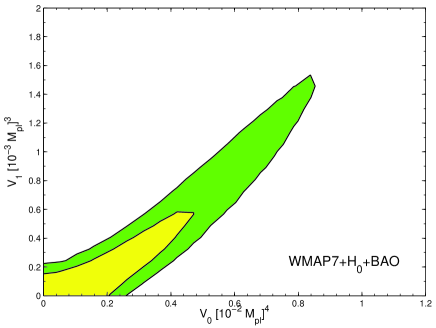
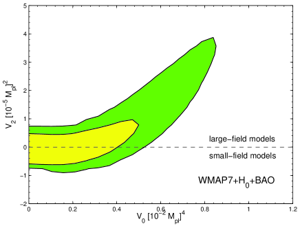
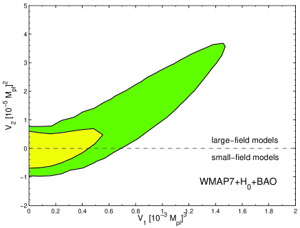
Figure 1 shows the two-dimensional joint marginalized constraints on , and at 68% and 95% confidence level (C.L.) from the 7-year WMAP data with Gaussian priors on and the distance ratios. We find upper limits on the potential energy, the first and second derivative of the potential:
| (9) |
at C.L.. Thus the upper limit on the energy scale of inflation is less than two orders of magnitude lower than the reduced Planck mass, which corresponds to the grand unified theory scale. We see that , which is consistent with our assumption that the Taylor series converges. Moreover, is almost five orders of magnitudes below the Planck scale, which confirms that the potential must be very flat, consistent with the assumption of slow-roll inflation. Another observation is that there is a strong degeneracy of the upper limits of all considered Taylor coefficients on . This stresses again how important the identification of the inflationary energy scale is for model building. We have also checked that , and are not degenerate with any of the other cosmological parameters.
IV Future constraints from Planck
In this section, following the approach described in Refs. per06 ; gal10 we generate synthetic data for the Planck experiment and then perform a systematic analysis on the simulated data. First of all, we assume a fiducial cosmological model: baryon density , cold dark matter density , the Hubble parameter , reionization optical depth , amplitude of scalar perturbation , scalar spectral index and tensor-to-scalar ratio . Given the fiducial cosmological model, one can use a Boltzmann code such as CAMB lew99 to calculate the power spectra for the temperature and polarization anisotropies , , and .
We assume that beam uncertainties are small and that uncertainties due to foreground removal are smaller than statistical errors. For an experiment with multiple channels with different beam width and sensitivity, the noise power spectrum can be approximated as kin98
| (10) | |||||
where is the root mean square of the instrumental noise per pixel for temperature (), -mode polarization () and -mode polarization (), and is the full width at half maximum of Gaussian beam for channel . Non-diagonal noise terms are expected to vanish since the noise contribution from different maps are uncorrelated. For Planck we combine only the , and GHz HFI channels, with beam width in arcminutes, temperature noise per pixel in and polarization noise per pixel in (see Ref. tau10 for the instrumental specifications of Planck).
Given the fiducial spectra and noise spectra , one can generate a random realization of using the following method per06
| (11) | |||||
| (12) | |||||
| (13) |
where and are Gaussian-distributed random numbers with unit variance. Then one can reconstruct the power spectra of the mock data by
| (14) |
Once simulated data are produced we perform a Monte Carlo analysis through the effective defined as eas04
| (15) | |||||
where is the sky fraction sampled by the experiment after foregrounds removal. For the Planck data we choose , corresponding to a Galactic cut.
We consider the , and power spectra on scales with . A measurement of the amplitude of the primordial gravitational waves would allow a direct determination of the inflationary energy scale. Both the primordial gravitational waves and the weak gravitational lensing of the -mode polarization are sources of -mode polarization zal98 . On large scales, the contributions to the -mode signal mainly come from the primordial gravitational waves generated by inflation. The effect of the weak gravitational leansing on the -mode power spectrum ultimately dominates on small scales. For the fiducial model with the -mode signal generated by the weak gravitational lensing dominates above and peaks at . We consider the power spectrum up to the peak of the spectrum at since the uncertainty in arising from instrument noise becomes large on smaller scales.
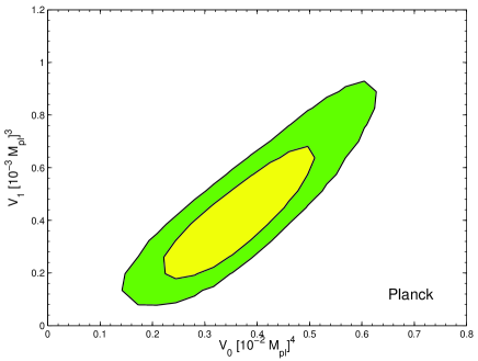
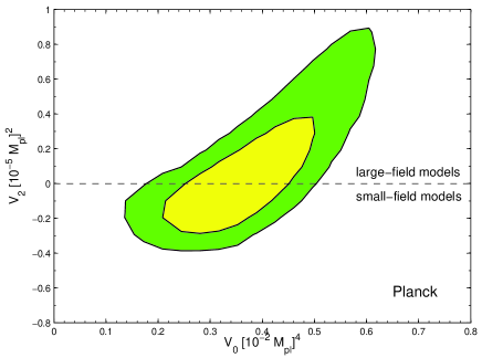
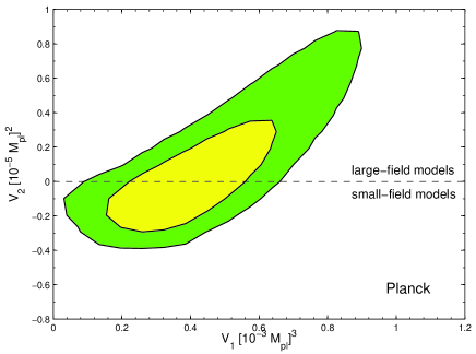
Figure 2 shows the forecast constraints on , and at 68% and 95% C.L. from the simulated Planck data in the case of . As expected, it illustrates dramatically how Plank can break degeneracies between the potential parameters if the scalar-to-tensor ratio is tightly constrained by Planck. The marginalized (68%) errors on , and are 0.099 , 0.18 and 0.27 , respectively. As we can see, Planck can place strong constraints on the inflationary energy scale, which would provide a firm observational link with the physics of the early Universe. The primordial gravitational waves could be detected at C.L. based on our fiducial cosmological model with . In order to distinguish the large-field models from the small-field models it is important to detect the sign of the second derivative of the potential. The analysis of our fiducial cosmological model indicates that Planck will not be able to distinguish these models.
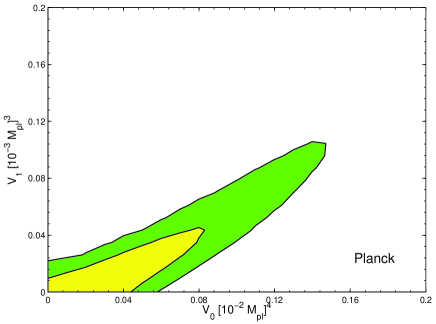
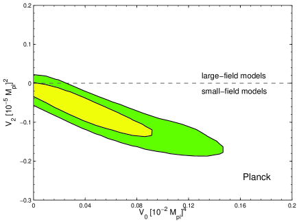
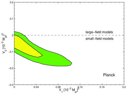
What about the forecast constraints from Planck if ? Here we show the case of . The fiducial values of the other parameters are taken to be the WMAP5 maximum likelihood values kom08 . Figure 3 shows the forecast constraints on the potential parameters at 68% and 95% C.L. from the simulated Planck data in the case of . We can see that in this case Planck only provides the upper limits on the energy scale of inflation as WMAP7 does. It is implied that Planck fails to detect the primordial gravitational waves if the tensor-to-scalar ratio is less than one percent. As shown in Figure 3, in this case “small-field” models would obviously be favored by data compared to the case of . It can be understood from Eq. (8). If and , the second term dominates over the first one in the bracket. Therefore, a red tilt of the power spectrum of curvature perturbations leads to a negative second derivative of the potential. The upper limits achievable by Planck are
| (16) |
at 95% C.L..
V Conclusions
In this paper we have placed observational constrains on the potential energy scale, the first and second derivative of the potential by using the 7-year WMAP data, combined with the latest distance measurements from the baryon acoustic oscillations in the distribution of galaxies and measurement of the present-day Hubble constant from supernova data. A previous upper limit from the first WMAP data release, combined with large scale structure data from the 2dF galaxy redshift survey found GeV at 90% C.L. lea03 ; sch04 . Our new upper limit on the energy scale of inflation is only slightly stronger GeV at 95% C.L., and shows a degeneracy with the upper limit on the first derivative of the inflaton potential, GeV at 95% C.L.. Adding information on the power spectrum of large scale structure, the limit would be improved slightly fin10 . Both upper limits lie at the energy scale of grand unified theories and are consistent with scenarios in which inflation starts very close to the Planck scale. However, a scenario in which there is just enough inflation RS in order to solve the horizon and flatness problems but for all field values cannot be excluded, nor can false vacuum initial conditions be excluded. Latter scenarios can be constrained by a lower limit on the reheating temperature of the Universe. A recent analysis MR of the 7-year WMAP data finds that the so-called reheating parameter, fully characterizing the inflationary reheating epoch, is constrained by data, which yields lower bounds on the reheating temperature, typically , dependent on inflation scenarios.
The Planck experiment will soon provide a very accurate measurements of CMB temperature and polarization anisotropies. Using the Monte Carlo simulation approach, we have presented forecasts for improved constrains from Planck. Our results indicate that the degeneracies between the potential parameters are broken because of the improved constraint on the tensor-to-scalar ratio from Planck. Besides Planck also EBEX, a balloon-borne CMB polarization experiment, has good chances to significantly improve our understanding of inflation rei07 .
In our analysis, we adopt the three-parameter parametrization of the potential for the case of a single, minimally coupled inflaton field. To leading order in the slow-roll approximation, it is consistent to expand the potential only to quadratic order, because the third derivative corresponds to higher-order slow-roll parameters. The advantage of the model-independent parametrization is that we could discriminate inflationary models by detecting the sign of the second derivative of the potential. If we drop one of the other assumptions, e.g. by means of a coupling of the inflaton and a Gauss-Bonnet term, we change the prediction of the tensor-to-scalar ratio GS and thus the limit on the inflationary energy scale.
It is quite surprising that one of the most fundamental questions in the context of inflationary cosmology, namely what is the energy scale of the observable part of the inflationary expansion, has received relatively little attention in the attempt to extract information from cosmic data. We hope that we can convince the reader, that even without a detection of tensor fluctuations, some interesting upper limits on three parameters can be extracted and that our analysis turns out to be fully self-consistent.
Acknowledgments
We thank H.-T. Ding and L. Perotto for useful discussions. Our numerical analysis was performed on the HPC cluster of the RWTH Aachen. This work was supported in part by the Alexander von Humboldt Foundation. YZZ is partially supported by National Basic Research Program of China under Grant No:2010CB832805. We used CosmoMC and CAMB. We also acknowledge the use of WMAP data from LAMBDA server.
References
- (1) J. E. Lidsey, A. R. Liddle, E. W. Kolb, E. J. Copeland, T. Barreiro and M. Abney, Rev. Mod. Phys. 69, 373 (1997) [arXiv:astro-ph/9508078].
- (2) B. A. Bassett, S. Tsujikawa and D. Wands, Rev. Mod. Phys. 78, 537 (2006) [arXiv:astro-ph/0507632]; K. A. Malik and D. Wands, Phys. Rept. 475, 1 (2009) [arXiv:0809.4944].
- (3) E. Komatsu, et al., Astrophys. J. Suppl. 180, 330 (2009) [arXiv:arXiv:0803.0547].
- (4) E. Komatsu, et al., arXiv:arXiv:1001.4538.
- (5) A. R. Liddle and M. S. Turner, Phys. Rev. D 50, 758 (1994) [arXiv:astro-ph/9402021]; M. Turner and M. White, Phys. Rev. D 53, 6822 (1996) [arXiv:astro-ph/9512155]; E. J. Copeland, I. J. Grivell, E. W. Kolb and A. R. Liddle, Phys. Rev. D 58, 043002 (1998) [arXiv:astro-ph/9802209]; I. J. Grivell and A. R. Liddle, Phys. Rev. D 61, 081301 (2000) [arXiv:astro-ph/9906327]; J. Lesgourgues and W. Valkenburg, Phys. Rev. D 75, 123519 (2007) [arXiv:astro-ph/0703625].
- (6) A. R. Liddle, Phys. Rev. D 49, 739 (1994) [arXiv:astro-ph/9307020].
- (7) S. M. Leach and A. R. Liddle, Phys. Rev. D 68, 123508 (2003) [arXiv:astro-ph/0306305].
- (8) D. J. Schwarz and C. A. Terrero-Escalante, JCAP 0408, 003 (2004) [arXiv:astro-ph/0403129].
- (9) A. R. Liddle, D. Parkinson, S. M. Leach and P. Mukherjee, Phys. Rev. D 74, 083512 (2006) [arXiv:astro-ph/0607275]; J. Martin and C. Ringeval, JCAP 0608, 009 (2006) [arXiv:astro-ph/0605367].
- (10) C. Destri, H. J. de Vega and N. G. Sanchez, Phys. Rev. D 77, 043509 (2008) [arXiv:astro-ph/0703417]; D. Boyanovsky, C. Destri, H. J. de Vega and N. G. Sanchez, Int. J. Mod. Phys. A 24, 3669 (2009) [arXiv:0901.0549].
- (11) E. W. Kolb, arXiv:hep-ph/9910311.
- (12) F. L. Bezrukov and M. Shaposhnikov, Phys. Lett. B 659, 703 (2006) [arXiv:hep-ph/0710.3755].
- (13) A. Lewis and S. Bridle, Phys. Rev. D 66, 103511 (2002) [arXiv:astro-ph/0205436].
- (14) A. G. Riess, et al., Astrophys. J. 699, 539 (2009) [arXiv:0905.0695].
- (15) W. J. Percival, et al., Mon. Not. Roy. Astron. Soc. 401, 2148 (2010) [arXiv:0907.1660].
- (16) L. Perotto, J. Lesgourgues, S. Hannestad, H. Tu and Y. Y. Y. Wong, JCAP 0610, 013 (2006) [arXiv:astro-ph/0606227].
- (17) S. Galli, et al., arXiv:1005.3808.
- (18) A. Lewis, A. Challinor and A. Lasenby, Astrophys. J. 538, 473 (2000) [arXiv:astro-ph/9911177].
- (19) W. H. Kinney, Phys. Rev. D 58, 123506 (1998) [arXiv:astro-ph/9806259].
- (20) J. A. Tauber, et al., A&A 520, A1 (2010).
- (21) R. Easther, W. H. Kinney and H. Peiris, JCAP 0505, 009 (2005) [arXiv:astro-ph/0412613].
- (22) M. Zaldarriaga and U. Seljak, Phys. Rev. D 58, 023003 (1998) [arXiv:astro-ph/9803150]; A. Lewis, Phys. Rev. D 71, 083008 (2005) [arXiv:astro-ph/0502469].
- (23) F. Finelli, J. Hamann, S. M. Leach and J. Lesgourgues, JCAP 1004, 011 (2010) [arXiv:0912.0522].
- (24) E. Ramirez and D. J. Schwarz, Phys. Rev. D 80, 023525 (2009) [arXiv:0903.3543].
- (25) J. Martin and C. Ringeval, Phys. Rev. D 82, 023511 (2010) [arXiv:1004.5525].
- (26) B. Reichborn-Kjennerud, et al., arXiv:1007.3672.
- (27) Z. K. Guo and D. J. Schwarz, Phys. Rev. D 80, 063523 (2009) [arXiv:0907.0427]; Z. K. Guo and D. J. Schwarz, Phys. Rev. D 81, 123520 (2010) [arXiv:1001.1897]; J. Moldenhauer, M. Ishak, J. Thompson and D. A. Easson, Phys. Rev. D 81, 063514 (2010) [arXiv:1004.2459]; M. Satoh, arXiv:1008.2724.