Optimal Distributed P2P Streaming under Node Degree Bounds

Abstract

We study the problem of maximizing the broadcast rate in peer-to-peer (P2P) systems under node degree bounds, i.e., the number of neighbors a node can simultaneously connect to is upper-bounded. The problem is critical for supporting high-quality video streaming in P2P systems, and is challenging due to its combinatorial nature. In this paper, we address this problem by providing the first distributed solution that achieves near-optimal broadcast rate under arbitrary node degree bounds, and over arbitrary overlay graph. It runs on individual nodes and utilizes only the measurement from their one-hop neighbors, making the solution easy to implement and adaptable to peer churn and network dynamics. Our solution consists of two distributed algorithms proposed in this paper that can be of independent interests: a network-coding based broadcasting algorithm that optimizes the broadcast rate given a topology, and a Markov-chain guided topology hopping algorithm that optimizes the topology. Our distributed broadcasting algorithm achieves the optimal broadcast rate over arbitrary P2P topology, while previously proposed distributed algorithms obtain optimality only for P2P complete graphs. We prove the optimality of our solution and its convergence to a neighborhood around the optimal equilibrium under noisy measurements or without time-scale separation assumptions. We demonstrate the effectiveness of our solution in simulations using uplink bandwidth statistics of Internet hosts.

TABLE I: Summary and comparison of previous work and this work for maximizing P2P broadcast rate.

References	General	Arbitrary Node	Exact or $1-\epsilon$	Distributed
	Overlay Graph?	Degree Bound?	Optimality?	Solution?
Mutualcast [1] and the algorithms in [2, 3]	$\times$	$\times$	$\mathbf{\checkmark}$	$\mathbf{\checkmark}$
Iterative in [4, 5]	$\mathbf{\checkmark}$	$\times$	$\mathbf{\checkmark}$	$\times$
CoopNet/SplitStream [6, 7]	$\times$	$\mathbf{\checkmark}$	$\times$	$\times$
ZIGZAG [8], PRIME [9]	$\mathbf{\checkmark}$	$\mathbf{\checkmark}$	$\times$	$\mathbf{\checkmark}$
Cluster-tree [10]	$\times$	$\mathbf{\checkmark}$	conditionally optimal ∗	$\times$
This paper	$\mathbf{\checkmark}$	$\mathbf{\checkmark}$	$\mathbf{\checkmark}$	$\mathbf{\checkmark}$

$\;{}^{*}$ The Cluster-Tree algorithm is $(1-\epsilon)$-optimal with high probability if the node degree bound is $O\left(\log N\right)$.

I Introduction

Peer-to-peer (P2P) systems have provided a scalable and cost effective way for streaming video in the past decade. Recent studies [11, 12, 13, 14], however, indicate that the practical performance of P2P streaming systems can be far from their theoretical optimal.

There have been work studying the performance limit of P2P systems to understand and unleash their potential. One focus is on the streaming capacity problem [15] in P2P live streaming systems , i.e., maximizing the streaming rate subject to the peering and overlay topology constraints. The problem is critical for supporting high-quality video, which is determined by the streaming rate, in P2P live streaming systems. In this paper, we focus on the broadcast scenario where all peers in the system are receivers.

The case of unconstrained peering on top of a complete graph is well studied, where the maximum broadcast rate is derived in several papers [3, 1, 16, 2, 17]. The case of unconstrained peering over general graph can also be addressed by using a centralized solution[5].

The streaming capacity problem becomes NP-Complete over general graph with node degree bounds [10]. Node degree is defined as the number of simultaneous active connections that a node maintains with its neighbors. Due to connection overhead costs, it is necessary to limit the number of simultaneous connections a peer can maintain. This naturally bounds the node degrees in P2P systems. For instance, in practical systems such as PPLive [18], the total number of neighbors of a node is usually bounded around 200, and the number of active neighbors of a node is usually bounded by 10-15 [15]. In such large P2P systems with hundreds of thousands of peers, the system topology is not a complete graph.

There has been work studying this challenging problem of maximizing streaming rate under node degree bounds and over general P2P graph. SplitStream/CoopNet [6, 7], ZIGZAG [8], PRIME [9] and most practical systems (such as PPLive [18] and UUSee [19]) bound node degree but do not provide rate optimality guarantee. Recently, the authors in [10] proposed a centralized Cluster-Tree algorithm that achieves near-optimal broadcast rate with high probability over complete graph, under the assumption that the node degree bound is at least logarithmic in the size of the network. A summary and comparison of previous work and this work are in Table I.

Despite of these exciting results, the following two important questions remain open:

• What is the maximum broadcast rate under arbitrary node degree bounds, and over general P2P overlay graph?

• How to achieve the maximum broadcast rate in a distributed manner?

Systems running distributed algorithms, compared with those running centralized algorithms, are more adaptable to peer churn and network dynamics.

In this paper, we answer the above two questions and make the following contributions:

• We provide the first distributed solution that achieves a broadcast rate arbitrarily close to the optimal under arbitrary node degree bounds, and over arbitrary overlay graph. Our solution runs on individual nodes and utilizes only the information from their one-hop neighbors.

Our solution consists of the following two algorithms that can be of independent interests.

• We propose a distributed broadcasting algorithm that achieves the optimal broadcast rate over arbitrary overlay graph. Previous distributed P2P broadcasting algorithms are optimal only for complete overlay graph [2, 1, 3]. Our algorithm is based on network coding and utilizes back-pressure arguments.

• We also propose a distributed algorithm that optimizes the topology. In this algorithm, each node hops among their possible set of neighbors towards the best peering configuration. Our algorithm is inspired by a set of log-sum-exp approximation and Markov chain based arguments expounded in [20].

• We prove the optimality of the overall solution. We also prove its convergence to a neighborhood around the optimal equilibrium in the presence of noisy measurements or without time-scale separation assumptions. We demonstrate the effectiveness of our solution in simulations using uplink bandwidth statistics of Internet hosts.

II Problem Formulation

II-A Settings and Notations

We model the P2P overlay network as a general directed graph $G=(V,E)$, where $V$ denotes the set of nodes and $E$ denotes the set of links. Each link in the graph corresponds to a TCP/UDP connection between two nodes. Let $N_{v}$ denote the neighbor set of node $v\in V$ in the graph. Each node $v\in V$ is associated with an upload capacity $C_{v}\geq 0$. We assume there is no constraint on the downloading rate for each node $v\in V$. This assumption can be partly justified by the empirical observation that as residential broadband connections with asymmetric upload and download rates become increasingly dominant, bottlenecks typically are at the uplinks of the access networks rather than in the middle of the Internet.

As such, P2P networks have capacity limits on the nodes instead of links. This is different from traditional underlay networks where the capacity limits are on the links.

We focus on the single-source streaming scenario, i.e., a source $s$ broadcasts a continuous stream of contents to the entire network; we denote its receiver set as $R\triangleq V-\{s\}$.

We consider the peering constraints that each node has a degree bound $B_{v}$, i.e., it can only exchange streaming content with up to a $B_{v}$ number of neighbors simultaneously due to connection overhead cost. We allow different nodes to have different degree bounds. Fig. 1 shows four sample peering configurations of a $5$-node network with node degree bound $3$ for each node.

Figure 1: Peering configuration examples for a $5$-node network with node degree bound $3$ for each node.

Let $\mathcal{F}$ denote the set of all feasible peering configurations over graph $G$ under node degree bounds. Given a configuration $f\in\mathcal{F}$, we obtain a connected sub-graph of $G$ that satisfies the node degree bound constraints. We denote this sub-graph as $G_{f}=\left(V,E_{f}\right)$, where $E_{f}$ represents the set of links in this sub-graph. We denote $N_{v,f}$ as the set of node $v$’s neighbors in this sub-graph. We have $|N_{v,f}|\leq B_{v}$ where $|\cdot|$ represents the size of a set.

II-B Problem Formulation and Our Approach

For a configuration $f\in\mathcal{F}$, let $x_{f}$ be the maximum achievable broadcast rate under $f$, i.e., the highest rate at which every node in the system can receive the streaming content simultaneously. The problem of maximizing broadcast rate under node degree bounds can be formulated as follows:

$$\mathbf{MRC:} \max_{f\in\mathcal{F}} x_{f}.$$ (1)

This problem is combinatorial in nature which is known to be NP-complete [10], and there is no efficient approximate solution to the problem even in a centralized manner.

In this paper, we address this problem by providing a distributed solution. In particular, we first develop a distributed broadcasting algorithm that can achieve $x_{f}$ under arbitrary $f\in\mathcal{F}$. We then design a distributed algorithm that optimizes towards the best peering configurations. They operate in tandem to achieve a close-to-optimal broadcast rate under arbitrary node degree bounds, and over arbitrary overlay graph. We elaborate on these two algorithms in the following two sections.

III The Proposed Distributed Broadcasting Algorithm

By exploiting network coding [21], we design a back-pressure based distributed broadcasting algorithm. Back-pressure type algorithm is proposed initially in [22]. This type of algorithms select a subset of queues in the system with the maximum back-pressures and serve these queues subject to resource constraints, where back-pressure is defined as the difference between the queue at the local node and that of its downstream nodes. Back-pressure algorithm design has found applications in many network resource allocation domains [23], [24], [25]. In this paper, we apply this method for the first time to design distributed P2P broadcasting algorithm. Our algorithm can achieve the maximum broadcast rate over arbitrary P2P topology.

III-A Routing vs. Network Coding

In P2P systems, there are two approaches for broadcasting contents: one is based on routing [26], in which nodes only store and forward packets; and the other is based on network coding [21], [26], in which a node is also allowed to mix information and output data as functions of the data it received. Some commercial P2P systems are built upon routing-based approach (e.g., PPLive [18]), and some are based on network coding (e.g., UUSee [19, 27]). It is known that both routing and network coding approaches can achieve optimal broadcast rate over arbitrary P2P graph [17, 2]. Compared to routing-based approach, the network-coding based approach introduces additional packet header overhead for carrying coding coefficients (e.g., $3\%$ extra overhead according to [29]) and computation complexity for encoding and decoding (e.g., [13, 27] discuss how to keep the complexity low). However, the network-coding based approach is robust to peer dynamics since there is no need for constructing and maintaining the spanning trees. In this section, we design a distributed broadcasting algorithm based on network coding that is robust to dynamics. In Section VII, we will discuss how the overall problem can be solved by using centralized solutions when only routing is allowed.

III-B Network Coding Based Formulation

According to the Max-Flow-Min-Cut theorem, a data transmission of rate $z$ between source $s$ and a receiver $d$ is feasible if and only if there exists a flow, denoted as $\boldsymbol{f}^{d}$, satisfying the following flow conservation constraints:

$$\sum_{u\in in(v)}f_{uv}^{d} \leq \sum_{u\in out(v)}f_{vu}^{d},\;\;\forall v\in R-\left\{d\right\},$$ (2)

$$z \leq \sum_{u\in out(s)}f_{su}^{d},$$ (3)

$$0 \leq \boldsymbol{f}^{d},$$ (4)

where $in(v)\triangleq\{u|(u,v)\in E_{f}\}$ is the set of nodes sending content to $v$ under configuration $f$, and $out(v)\triangleq\{u|(v,u)\in E_{f},u\neq s\}$ is the set of nodes receiving content from $v$.

A powerful theorem established in [21] states that a multicast or broadcast rate $z$ from $s$ to a set of receivers is achievable if and only if $z$ is feasible for $s$ and any receiver $d$. This is a strong result as it says that if the network can support a unicast rate of $z$ between $s$ and any receiver assuming other receivers’ traffic is absent, then it can support a multicast rate of $z$ to all the receivers simultaneously. Such rate $z$ can be achieved by every node in the network performing network coding [21]. Further, authors in [30, 29] show that it is sufficient to perform random linear network coding.

In random linear network coding, by independently and randomly choosing a set of coding coefficients from a finite field, each node sends out the coded packet as a linear combination of the node’s received packets. The combination information is specified by a coefficient vector in the packet header, which is updated by applying the same linear transformations as to the data. When one node receives a full set of linearly independent coded packets, it can decode and recover the original packets. In this paper, we focus on the distributed algorithm design. The discussions of decoding probability and implementation details can be found in [30, 29].

Under the setting of network coding, we can consider $\boldsymbol{f}^{d}$ as a “virtual” information flow between $s$ and $d$. Multiple information flows “piggyback” together to transmit over the physical links. The actual physical rate over a physical link is only the maximum rate of individual information flows passing over it. Let $g_{uv}$ be the physical flow rate over a link $(u,v)\in E_{f}$, then we have $f_{uv}^{d}\leq g_{uv}$ for all $d\in R$.

With the above understanding, we formulate the problem of maximizing broadcast rate under configuration $f$ as follows:

$$\mathbf{MP:} \underset{z,\boldsymbol{f,g}\geq 0}{\max}U(z)$$ (5)

s.t. $$\!\!\!\sum_{u\in in(v)}f_{uv}^{d}+z\mathbbm{1}_{\left\{v=s\right\}}\leq\sum_{u\in out(v)}\!\!\!f_{vu}^{d},\forall v\in V-\{d\},d\in R,$$ (8)

$$f_{vu}^{d}\leq g_{vu},\forall v\in V,\forall u\in out(v),d\in R,$$

$$\!\!\!\sum_{u\in out(v)}g_{vu}\leq C_{v},\forall v\in V,$$

where $U\left(z\right)$ is a twice-differentiable strictly concave utility function, $\mathbbm{1}_{\{\cdot\}}$ denotes the indicator function. The constraints in (8) describe the flow conservation requirements. The constraints in (8) come from the piggybacking property of information flows. The node upload capacity constraints are in (8). The problem $\mathbf{MP}$ is a convex problem. All feasible broadcast rates must satisfy the constraints in (8)-(8) and are achievable by using random linear network coding.

III-C Algorithm Design via Lagrange Decomposition

To proceed, we first relax the first set of constraints in (8) in problem $\mathbf{MP}$ to obtain a partial Lagrangian as follows:

$$L(z,\boldsymbol{f,g,\lambda})$$

$$= U(z)-\sum_{v\in V-\{d\}}\sum_{d\in R}\lambda_{v,d}\left(\sum_{u\in in(v)}f_{uv}^{d}+z\mathbbm{1}_{\left\{v=s\right\}}-\sum_{u\in out(v)}f_{vu}^{d}\right)$$

$$= U(z)-\sum_{v\in V}\sum_{d\in R}\lambda_{v,d}\left(\sum_{u\in in(v)}f_{uv}^{d}+z\mathbbm{1}_{\left\{v=s\right\}}-\sum_{u\in out(v)}f_{vu}^{d}\right),$$ (9)

where $\lambda_{v,d},v\in V-\{d\},d\in R$ are Lagrange multipliers, $\lambda_{d,d}=0,\forall d\in R$, and $\sum_{u\in in(s)}f_{us}^{d}=0$.

The strong duality holds for problem $\mathbf{MP}$ since the Slater conditions are satisfied [31]. Therefore, we can solve problem $\mathbf{MP}$ by finding the saddle points of $L(z,\boldsymbol{f,g,\lambda})$.

Noticing that

$$\sum_{v\in V}\sum_{d\in R}\lambda_{v,d}\,z\mathbbm{1}_{\left\{v=s\right\}}=z\sum_{d\in R}\lambda_{s,d}$$ (10)

and

$$\sum_{v\in V}\sum_{d\in R}\lambda_{v,d}\left(\sum_{u\in in(v)}f_{uv}^{d}-\sum_{u\in out(v)}f_{vu}^{d}\right)=\sum_{d\in R}\sum_{v\in V}\sum_{u\in out(v)}f_{vu}^{d}(\lambda_{u,d}-\lambda_{v,d}),$$ (11)

we can find the saddle points of $L(z,\boldsymbol{f,g,\lambda})$ by solving the following problem successively in $z,\boldsymbol{f},\boldsymbol{g},\boldsymbol{\lambda}$:

$$\mathbf{\min_{\boldsymbol{\lambda}\geq 0}} \left(\max_{z\geq 0}(U(z)-z\sum_{d\in R}\lambda_{s,d})+\max_{\boldsymbol{f,g}\geq 0}\sum_{d\in R}\sum_{v\in V}\sum_{u\in out(v)}f_{vu}^{d}(\lambda_{v,d}-\lambda_{u,d})\right)$$ (12)

$$\;\;\;\;\;\;\mbox{s.t.}\;\eqref{eq:MPC2}-\eqref{eq:MPC3}.$$

Given $\boldsymbol{\lambda}$ and $z$, we consider the following scheduling subproblem on $\boldsymbol{f,g}$:

$$\mathbf{SSP:}\max_{\boldsymbol{f,g}\geq 0} \sum_{d\in R}\sum_{v\in V}\sum_{u\in out(v)}f_{vu}^{d}(\lambda_{v,d}-\lambda_{u,d})$$

s.t. $$\eqref{eq:MPC2}-\eqref{eq:MPC3}.$$

The above linear programming problem has a structure that allows us to solve it distributedly. The first observation is that if an optimal $\boldsymbol{g}^{*}$ is given, then an optimal $\boldsymbol{f}^{*}$ can be obtained as follows: $\forall u,v\in V,d\in R$,

$$\left(f_{vu}^{d}\right)^{*}=\begin{cases}0,&\mbox{if }\lambda_{v,d}-\lambda_{u,d}\leq 0,\\ g_{vu}^{*},&\mbox{otherwise.}\end{cases}$$ (14)

As such, it is sufficient to study the following problem in $\boldsymbol{g}$:

$$\mathbf{\max_{\boldsymbol{g\geq 0}}} \sum_{v\in V}\sum_{u\in out(v)}g_{vu}\,w_{vu}$$

s.t. $$\sum_{u\in out(v)}g_{vu}\leq C_{v},\forall v\in V,$$

where

$$w_{vu}\triangleq\sum_{d\in R}[\lambda_{v,d}-\lambda_{u,d}]^{+},\;\forall(u,v)\in E_{f}.$$ (16)

denotes the aggregate back-pressure between two neighboring nodes $u$ and $v$, and $[\cdot]^{+}\triangleq\max(\cdot,0)$.

For any $v\in V$, let

$$u^{*}(v)\triangleq\arg\max_{u\in out(v)}w_{vu}$$ (17)

be one of its neighbors with the maximum back-pressure (breaking ties arbitrarily). Then one optimal solution for problem $\mathbf{SSP}$ is as follows:

$$\left(g_{vu}^{d}\right)^{*}=\begin{cases}C_{v},&\mbox{if }u=u^{*}(v),\\ 0,&\mbox{otherwise,}\end{cases}$$ (18)

and

$$\left(f_{vu}^{d}\right)^{*}=\begin{cases}0,&\mbox{if }\lambda_{v,d}-\lambda_{u,d}\leq 0,\\ g_{vu}^{*},&\mbox{otherwise.}\end{cases}$$ (19)

Given $\boldsymbol{f}^{*}$ and $\boldsymbol{g}^{*}$, primal-dual algorithms can be designed to adapt $z$ and $\boldsymbol{\lambda}$ to pursue the desired optimal solution.

We summarize the above analysis into a distributed algorithm including the following components:

Primal-dual Rate Control: we pursue the saddle point in $z$ and $\boldsymbol{\lambda}$ simultaneously as follows:

$$\begin{cases}\dot{z}=\alpha[U^{{}^{\prime}}(z)-\sum_{d\in R}\lambda_{s,d}]_{z}^{+},\\ \dot{\lambda}_{v,d}=k_{v,d}\left[\sum_{u\in in(v)}\left(f_{uv}^{d}\right)^{*}+z\mathbbm{1}_{v=s}\right.\\ \;\;\;\;\;\;\;\;\;\;\;\;\;\;\;\;\;\;\;\;\left.-\sum_{u\in out(v)}\left(f_{vu}^{d}\right)_{\lambda_{v,d}}^{*}\right]_{\lambda_{v,d}}^{+},&\forall v\in V-\{d\},d\in R,\\ \dot{\lambda}_{d,d}=\lambda_{d,d}=0,\;\;\;\forall d\in R,\end{cases}$$ (20)

where $\alpha$ and $k_{v,d}$ are positive step sizes, and the function

$$[b]_{a}^{+}=\begin{cases}\max(0,b),&a\leq 0,\\ b,&a>0.\end{cases}$$

Neighbor Scheduling, Content Scheduling, and Network Coding: Every node $v\in V$ maintains a queue storing packets that are intended for $d$. Whenever a transmission opportunity arises, node $v$ chooses one neighbor $u^{*}(v)$ with the maximum back-pressure according to (17).

If $w_{vu^{*}(v)}>0$, node $v$ sends packets to $u^{*}(v)$ at rate $C_{v}$. Every output packet is constructed as follows. Node $v$ chooses one packet from the head of each queue of $d$ if $\lambda_{v,d}-\lambda_{u^{*}(v),d}>0$, and output one random linear combination of these heard-of-queue packets. If otherwise $w_{vu^{*}(v)}\leq 0$ or there is no head-of-line packets to code, node $v$ does nothing.

We have the following observations.

• The Lagrangian variable $\lambda_{v,d}$ is proportional to the length of queue storing packets that are intended for receiver $d$. The back-pressure $w_{vu}$ measures the aggregate difference in the queues of all $d\in R$ between $v$ and $u$. The larger the back-pressure is, the more desperate node $u$ wants to receive data from $v$.

• Our algorithm can be implemented in a distributed manner. It only requires nodes to exchange information with its one-hop neighbors, and thus is robust to peer churn and system dynamics. When a new peer arrives, it connects to a set of neighbors, assigned by the streaming server or trackers. Then the peer starts exchanging streaming data with them following the strategy defined by our algorithm. When a peer leaves, its neighbors are informed and then close the connections. For the network coding operation, theoretically we need to adjust the size of field where the coding coefficients are chosen to make sure of the decoding probability when the number of nodes changes [32], [33]. While [29] and [13] show that in practice the finite field $\mathbb{F}_{2^{8}}$ or $\mathbb{F}_{2^{16}}$ is enough to have a sufficiently high decoding probability. Therefore, only local configuration changes corresponding to dynamics, which is easy to implement compared to centralized algorithms where typically global information is needed for whole configuration change (e.g., spanning trees reconstruction in spanning tree based solutions).

• Although our algorithm is designed for P2P broadcast scenarios, it also works for P2P multicast scenarios where helper nodes exist. The helper nodes simply also perform the operations described in (18)-(20). Our algorithm can be considered as the extension of the algorithm in [30] from link-capacity-limited underlay networks to node-capacity-limited overlay networks.

The following theorem characterize the convergence of the proposed algorithm.

Theorem 1

The algorithm in (18)-(20) converges to the optimal solution of problem $\mathbf{MP}$ globally asymptotically in time.

The proof utilizes standard Lyapunov arguments and a Lyapunov function for primal-dual algorithm, similar to those used in [17], [34]. The proof is relegated to Appendix -A.

Remark: We derive our algorithm and prove its convergence based on a fluid model formulation. It is also possible to obtain a similar back-pressure based distributed algorithm with packet-level dynamics taken into account and prove its stability, following a set of Lyapunov drift arguments elaborated in [35].

IV The Proposed Distributed Topology Hopping Algorithm

We recently proposed in [20] to use Markov chain as a principled approach in designing distributed algorithms for solving combinatorial network problems approximately. In particular, we show one can design distributed algorithms for a combinatorial network optimization problem in the following way. First, construct a special class of Markov chains with problem-specific steady-state distribution. Second, search for a Markov chain in this class that allows distributed implementation. If such Markov chain can be found, which is usually challenging and problem-specific, the distributed implementation directly yields a distributed algorithm for the problem.

In this paper, we follow the framework from [20] and design a distributed topology hopping algorithm for our problem (1). There are two steps in designing our algorithm under the Markov approximation framework [20]: log-sum-exp approximation and constructing problem-specific Markov chains that allows distributed implementation.

IV-A Log-Sum-Exp Approximation

First, the maximum broadcast rate can be approximated by a log-sum-exp function as follows:

$$\max_{f\in\mathcal{F}}\;x_{f}\,\approx\,\frac{1}{\beta}\log\left[\sum_{f\in\mathcal{F}}\exp\left(\beta x_{f}\right)\right],$$ (21)

where $\beta$ is a positive constant. Let $|\mathcal{F}|$ denote the size of the set $\mathcal{F}$, then the approximation accuracy is known as follows [20]:

$$0\leq\frac{1}{\beta}\log\left[\sum_{f\in\mathcal{F}}\exp\left(\beta x_{f}\right)\right]-\max_{f\in\mathcal{F}}\;x_{f}\leq\frac{1}{\beta}\log|\mathcal{F}|.$$ (22)

As $\beta$ approaches infinity, the approximation gap approaches zero. As discussed in [20], however, usually $\beta$ should not take too large values as there are practical constraints or convergence rate concerns in the algorithm design afterwards.

To better understand the log-sum-exp approximation, we associate with each configuration $f\in\mathcal{F}$ a probability $p_{f}$. Consider the following problem

$$\mathbf{MRC-EQ:}\max_{\boldsymbol{p\geq 0}} \sum_{f\in\mathcal{F}}p_{f}x_{f}$$ (23)

s.t. $$\sum_{f\in\mathcal{F}}p_{f}=1.$$ (24)

Its optimal value is $\max_{f\in\mathcal{F}}x_{f}$ and is obtained by setting the probability corresponding to one of the best configurations to be one and the rest probabilities to be zero. Hence, problem $\mathbf{MRC-EQ}$ is equivalent to the original problem $\mathbf{MRC}$.

On the other hand, according to [20] we have the following observations.

Theorem 2 (cf. [20])

The optimal value of the following optimization problem

$$\mathbf{MRC-\beta:} \max_{\boldsymbol{p}\geq 0}\sum_{f\in\mathcal{F}}p_{f}x_{f}-\frac{1}{\beta}\sum_{f\in\mathcal{F}}p_{f}\log p_{f}\;\;\;\;\;\;$$ (25)

$$\mbox{s.t.}\;\;\sum_{f\in\mathcal{F}}p_{f}=1$$ (26)

is given by $\frac{1}{\beta}\log\left[\sum_{f\in\mathcal{F}}\exp\left(\beta x_{f}\right)\right]$. The optimal solution of problem $\mathbf{MRC-\beta}$ is given by

$$p_{f}^{*}(\boldsymbol{x})=\frac{\exp\left(\beta x_{f}\right)}{\sum\limits_{f^{\prime}\in\mathcal{F}}\exp\left(\beta x_{f^{\prime}}\right)},\;\forall f\in\mathcal{F}.$$ (27)

As such, by the log-sum-exp approximation in (21), we obtain an approximate version of the maximum broadcast rate problem $\mathbf{MRC}$, off by an entropy term $-\frac{1}{\beta}\sum_{f\in\mathcal{F}}p_{f}\log p_{f}$. If we can time-share among different configurations according to the optimal solution $p_{f}^{*}(\boldsymbol{x})$ in (27), then we can solve the problem $\mathbf{MRC}$ approximately and obtain a close-to-optimal broadcast rate.

IV-B Markov Chain Guided Algorithm Design

We design a Markov chain with a state space being the set of all feasible peering configurations $\mathcal{F}$ and has a stationary distribution as $p_{f}^{*}(\boldsymbol{x})$ in (27). We implement the Markov chain to guide the system to optimize the configuration. As the system hops among configurations, the Markov chain converges and the configurations are time-shared according to the desired distribution $p_{f}^{*}(\boldsymbol{x})$.

The key lies in designing such Markov chain that allows distributed implementation. Since $p_{f}^{*}(\boldsymbol{x})$ in (27) is product-form, it suffices to focus on designing time-reversible Markov chains [20].

Let $f,f^{\prime}\in\mathcal{F}$ be two states of Markov chain, and denote $q_{f,f^{{}^{\prime}}}$ as the transition rate from state $f$ to $f^{{}^{\prime}}$. We have two degrees of freedom in designing a time-reversible Markov chain:

• The state space structure: we can add or cut direct transitions between any two states, given that the state space remains connected and any two states are reachable from each other.

• The transition rates: we can explore various options in designing $q_{f,f^{{}^{\prime}}}$, given that the detailed balance equation is satisfied, i.e.,

  $$p_{f}^{*}(\boldsymbol{x})q_{f,f^{{}^{\prime}}}=p_{f}^{*}(\boldsymbol{x})q_{f^{{}^{\prime}},f},\;\forall f,f^{\prime}\in\mathcal{F}.$$ (28)

  Satisfying the above equations guarantees the designed Markov chain has the desired stationary distribution as in (27).

Recall that for a node $v\in V$, the set of its neighbors under configuration $f$ is denoted by $N_{v,f}$. We call node in $N_{v,f}$ $v$’s in-use neighbor and node in $N_{v}\backslash N_{v,f}$ $v$’s not-in-use neighbor. For the ease of explanation, we further define $\mathcal{N}_{f}$ as the set of all the node-pairs under $f$, i.e., $\mathcal{N}_{f}=\{\{v,u\},\forall v\in V,u\in N_{v,f}\}$. Note we do not differentiate node pairs $\{u,v\}$ and $\{v,u\}$. As an example, for the peering configuration $f$ shown in Fig. 1(b), $\mathcal{N}_{f}$ is given by $\{\{s,1\},\{s,2\},\{s,4\},\{1,2\},\{1,4\},\{2,3\},\{3,4\}\}$.

In our Markov chain design, we first specify its state space structure as follows: we set the transition rate $q_{f,f^{\prime}}$ to be zero, unless $f$ and $f^{\prime}$ satisfy that $|\mathcal{N}_{f}\backslash\mathcal{N}_{f^{\prime}}|=1$ or $|\mathcal{N}_{f^{\prime}}\backslash\mathcal{N}_{f}|=1$. In other words, we only allow direct transitions between two configurations if such transitions correspond to a single node adding a new node in its in-use neighbor set or removing one in-use neighbor from its in-use neighbor set.

Second, given the state space structure of Markov chain, we design the transition rates to favor distributed implementation while satisfying the detailed balance equation in (28).

One possible option is to set $q_{f,f^{{}^{\prime}}}$ to be $\exp^{-1}(\beta x_{f})$. One way to implement this option is for every node to generate a timer according to its measured receiving rate and counts down accordingly. When the timer expires, the dedicated node performs the neighbor swapping and resets its timer. As simple as the implementation may sound, this option is expensive to implement. Once the peering configuration changes, the system needs to notify all the nodes to measure the new receiving rate and reset their timers accordingly. It is not clear how to implement such system-wide notification in a low-overhead manner.

In this paper, we design $q_{f,f^{{}^{\prime}}}$ and $q_{f^{\prime},f}$ as follows:

$$q_{f,f^{{}^{\prime}}}=\frac{1}{\exp(\tau)}\frac{\exp(\beta x_{f^{{}^{\prime}}})}{\exp(\beta x_{f})+\exp(\beta x_{f^{{}^{\prime}}})}$$ (29)

and

$$q_{f^{\prime},f}=\frac{1}{\exp(\tau)}\frac{\exp(\beta x_{f})}{\exp(\beta x_{f})+\exp(\beta x_{f^{{}^{\prime}}})},$$ (30)

where $\tau$ is a constant. It is straightforward to verify that detailed balance equation is satisfied. As will be clear in the next subsection, our choices of transition rates do not require coordination or notification among peers in its implementation.

IV-C Distributed Implementation

One distributed implementation of our designed Markov chain is briefly described as follows.

• Initialization: Each peer $v\in V$ randomly selects neighbors from its neighbor list $N_{v}$ under the node degree bound and builds connections with these selected neighbors.

• Step 1: Let $f$ denote the current configuration. Each node $v\in V$ generates an exponentially distributed random number independently with mean $\frac{2\exp(\tau)}{|N_{v}|}$, and counts down according to this number.

• Step 2: When the count-down expires, node $v$ measures its current receiving rate as an estimate of the broadcast rate $x_{f}$. Then with probability $\frac{|N_{v,f}|}{|N_{v}|}$ node $v$ goes to the Step 2a; with probability $\frac{|N_{v}|-|N_{v,f}|}{|N_{v}|}$, node $v$ goes to the Step 2b;

  • Step 2a: Node $v$ randomly selects one in-use neighbor in $N_{v,f}$ and removes it from $N_{v,f}$. Under the new peering configuration $f^{{}^{\prime}}$, node $v$ measures its receiving rate as an estimate of $x_{f^{{}^{\prime}}}$. With the estimates of $x_{f}$ and $x_{f^{{}^{\prime}}}$, peer $v$ stays in the new configuration $f^{{}^{\prime}}$ with probability $\frac{\exp(\beta x_{f^{{}^{\prime}}})}{\exp(\beta x_{f})+\exp(\beta x_{f^{{}^{\prime}}})}$, and switches back to $f$ with probability $1-\frac{\exp(\beta x_{f^{{}^{\prime}}})}{\exp(\beta x_{f})+\exp(\beta x_{f^{{}^{\prime}}})}$. Node $v$ then repeats Step 1.

  • Step 2b: Node $v$ randomly selects one not-in-use neighbor in $N_{v}\backslash N_{v,f}$. If the node degree of the selected not-in-use node is equal to the bound or $v$’s node degree is equal to the bound, node $v$ jumps back to Step 1 immediately. Otherwise, node $v$ adds this selected node into $N_{v,f}$. Under the new peering configuration $f^{{}^{\prime}}$, node $v$ measures its receiving rate as an estimate of $x_{f^{{}^{\prime}}}$. With the estimates of $x_{f}$ and $x_{f^{{}^{\prime}}}$, peer $v$ stays in the new configuration $f^{{}^{\prime}}$ with probability $\frac{\exp(\beta x_{f^{{}^{\prime}}})}{\exp(\beta x_{f})+\exp(\beta x_{f^{{}^{\prime}}})}$, and switches back to $f$ with probability $1-\frac{\exp(\beta x_{f^{{}^{\prime}}})}{\exp(\beta x_{f})+\exp(\beta x_{f^{{}^{\prime}}})}$. Node $v$ then repeats Step 1.

It is straightforward to summarize the above implementation into a distributed algorithm that runs on individual nodes and utilizes only the measurement from their one-hop neighbors. The correctness of the implementation is shown as follows:

Proposition 1

The implementation in fact realizes a time-reversible Markov chain with stationary distribution in (27).

The proof is relegated to Appendix -B.

Remarks: a) In Step 1, the generation of count-down timers does not depend on the receiving rate, thus the system does not need to notify the nodes about changes of peering configurations. b) With the above implementation, the system hops towards configurations with better broadcast rate probabilistically. For example, if $x_{f^{\prime}}>x_{f}$, then the system will be more likely to stay in configuration $f^{\prime}$ than in $f$, and vice versa. c) With large values of $\beta$, the system hops towards better configurations more greedily. However, this may as well lead to the system getting trapped in locally optimal configurations. Hence there is a trade-off to consider when setting the value of $\beta$. Moreover, the value of $\beta$ also affects the convergence rate of the time-reversible Markov chain to the desired stationary distribution. It is worth future investigation to further understand the impact of $\beta$. d) In the presence of peer dynamics, our algorithm incurs only simple actions based on local information. When a new peer arrives, a neighbor set and a neighbor list are assigned to it. The peer builds connections with the nodes in the neighbor set. Then the peer starts counting down as Step 1 and follows the strategy of our algorithm. When a peer leaves, we just eliminate it from the neighbor list of its previous neighbors and end up connections.

V Convergence Properties of Overall Solution

Algorithm 1 Broadcasting Algorithm

1:  The following procedure runs on each individual node independently.

2:  For the source $s$ and each time slot,

3:     $x\leftarrow\left[x+\alpha(U^{{}^{\prime}}(x)-\sum_{d\in R}\lambda_{s,d})\right]^{+}$

4:  For each node $v\in V$ and each time slot,

5:  $w^{*}\leftarrow 0$

6:  for $u\in out(v)$ do

7:     for for $d\in R$ do

8:        $w_{vu}\leftarrow w_{vu}+\mbox{max}(\lambda_{v,d}-\lambda_{u,d},0)$

9:     end for

10:     if $w_{vu}>w^{*}$ then

11:        $w^{*}\leftarrow w_{vu}$

12:        $u^{*}\leftarrow u$

13:     end if

14:  end for

15:  if $w_{vu^{*}}>0$ then

16:     for $d\in R$ do

17:        if $\lambda_{v,d}-\lambda_{u^{*},d}>0$ then

18:           $f_{vu^{*}}^{d}\leftarrow C_{v}$

19:        end if

20:     end for

21:  end if

22:  for $d\in R$ do

23:     $\lambda_{v,d}\leftarrow\left[\lambda_{vd}+k_{v,d}(\sum_{u\in in(v)}f_{uv}^{d}-\sum_{u\in out(v)}f_{vu}^{d})\right]^{+}$

24:  end for

Algorithm 2 Topology Hopping Algorithm

1:  The following procedure runs on each individual node independently. We focus on a particular node $v\in V$.

2:  procedure Initialization

• Initialize $N_{v}$, $B_{v}$; randomly connects to peers from $N_{v}$ under the degree bound.

• Generate a timer that follows exponential distribution with mean equal to $2\exp(\tau)/(|N_{v}|)$ and begin counting down.

3:  end procedure

4:   

5:  When the timer expires, invoke the procedure Transition.

6:  procedure Transition

7:     With probability $\frac{|N_{v,f}|}{|N_{v}|}$,

8:        $N_{o}\leftarrow N_{v,f}$;

9:        randomly remove one in-use neighbor from $N_{v,f}$;

10:        $x_{f^{{}^{\prime}}}\leftarrow\sum_{u\in in(v)}f_{uv}^{v}$;

11:        $N_{v,f}$ $\leftarrow$ $N_{o}$ with probability      $1-{\exp(\beta x_{f^{{}^{\prime}}})}/{\left(\exp(\beta x_{f})+\exp(\beta x_{f^{{}^{\prime}}})\right)}$;

12:        refresh the timer and begin counting down;

13:     With probability $1-\frac{|N_{v,f}|}{|N_{v}|}$,

14:        $N_{o}\leftarrow N_{v,f}$;

15:        randomly add one not-in-use neighbor $v^{{}^{\prime}}$ in      $N_{v}\backslash N_{v,f}$ to $N_{v,f}$;

16:        if $|N_{v,f}|=B_{v}$ or $|N_{v^{{}^{\prime}},f}|=B_{v^{{}^{\prime}}}$

17:           refresh the timer and begin counting down;

18:        end if

19:        $x_{f^{{}^{\prime}}}\leftarrow\sum_{u\in in(v)}f_{uv}^{v}$;

20:        $N_{v,f}$ $\leftarrow$ $N_{o}$ with probability      $1-{\exp(\beta x_{f^{{}^{\prime}}})}/{\left(\exp(\beta x_{f})+\exp(\beta x_{f^{{}^{\prime}}})\right)}$;

21:        refresh the timer and begin counting down;

22:  end procedure

We have designed the distributed broadcasting algorithm in Section III and the Markov chain guided topology hopping algorithm in Section IV. The pseudocodes of each algorithm are shown in Algorithm 1 and Algorithm 2 respectively. Both algorithms are simple to implement, run on each individual node, and only require nodes to exchange information with their neighbors.

If the broadcasting algorithm converges instantaneously, i.e., time-scale separation assumption holds, then we can obtain the accurate value of $x_{f}$ for any configuration $f\in\mathcal{F}$. Transiting based on the accurate $x_{f}$, the designed Markov chain will converges to the desired stationary distribution in (27). Hence by operating these two algorithms in tandem, we obtain a close-to-optimal broadcast rate under arbitrary node degree bounds, and over arbitrary overlay graph. The optimality gap is characterized in (22).

In practice, however, it is possible to obtain only an inaccurate measurement or estimate of $x_{f}$. These inaccuracies root in two sources. One is the noisy measurements of the maximum broadcast rates given the configuration. The other is the fast state transition of Markov chain, i.e., the Markov chain transits before the underlying broadcasting algorithm converges and thus it transits based on inaccurate observations of the broadcast rates.

Consequently, the topology hopping Markov chain may not converge to the desired stationary distribution $p_{f}^{*}(\boldsymbol{x})$. This observation motivates our following study on the convergence of Markov chain in the presence of inaccurate transition rates.

For each configuration $f\in\mathcal{F}$ with broadcast rate $x_{f}$, we assume its corresponding inaccurate observed rate belongs to the bounded region $\left[-\Delta_{f},\Delta_{f}\right]$. $\Delta_{f}$ is the inaccuracy bound and can be different for different $f$.

For easy explanation of our approach, we further assume the observed broadcast rate for configuration $f$ only takes one of the following $2n_{f}+1$ discrete values:

$$\left[x_{f}-\Delta_{f},\ldots,x_{f}-\frac{1}{n_{f}}\Delta_{f},x_{f},x_{f}+\frac{1}{n_{f}}\Delta_{f},\ldots,x_{f}+\Delta_{f}\right],$$

where $n_{f}$ is a positive constant. Further, with probability $\eta_{j,f}$, the observed broadcast rate takes value $x_{f}+\frac{j}{n_{f}}\Delta_{f}$, $\forall j\in\{-n_{f},\ldots,n_{f}\}$ and $\sum_{j=-n_{f}}^{n_{f}}\eta_{j,f}=1$.

With the inaccurate observed broadcast rates, the topology hopping behaves as follows. Suppose the current configuration is $f$ and the observed broadcast rate is $x_{f}+\frac{j}{n_{f}}\Delta_{f}$, where $j\in\{-n_{f},\ldots,n_{f}\}$. After some count-down process, the system hops to a new configuration $f^{\prime}$ and probes its broadcast rate. In configuration $f^{\prime}$, the broadcast rate is observed as $x_{f^{\prime}}+\frac{j^{\prime}}{n_{f^{\prime}}}\Delta_{f^{\prime}},j^{\prime}\in\{-n_{f^{\prime}},\ldots,n_{f^{\prime}}\}$. The system stays in the new configuration $f^{\prime}$ with probability

$$\frac{\exp(\beta(x_{f^{\prime}}+\frac{j^{\prime}}{n_{f^{\prime}}}\Delta_{f^{\prime}}))}{\exp(\beta(x_{f^{\prime}}+\frac{j^{\prime}}{n_{f^{\prime}}}\Delta_{f^{\prime}}))+\exp(\beta(x_{f}+\frac{j}{n_{f}}\Delta_{f}))},$$

and switches back to configuration $f$ with probability

$$1-\frac{\exp(\beta(x_{f^{\prime}}+\frac{j^{\prime}}{n_{f^{\prime}}}\Delta_{f^{\prime}}))}{\exp(\beta(x_{f^{\prime}}+\frac{j^{\prime}}{n_{f^{\prime}}}\Delta_{f^{\prime}}))+\exp(\beta(x_{f}+\frac{j}{n_{f}}\Delta_{f}))}.$$

By arguments similar to the proof of Proposition $1$, the transition rate from configuration $f$ with broadcast rate $x_{f}+\frac{j}{n_{f}}\Delta_{f}$ to configuration $f^{\prime}$ with broadcast rate $x_{f^{\prime}}+\frac{j^{\prime}}{n_{f^{\prime}}}\Delta_{f^{\prime}}$ is given by

$$\frac{\eta_{j^{\prime},f^{\prime}}}{\exp(\tau)}\cdot\frac{\exp(\beta(x_{f^{\prime}}+\frac{j^{\prime}}{n_{f^{\prime}}}\Delta_{f^{\prime}}))}{\exp(\beta(x_{f^{\prime}}+\frac{j^{\prime}}{n_{f^{\prime}}}\Delta_{f^{\prime}}))+\exp(\beta(x_{f}+\frac{j}{n_{f}}\Delta_{f}))}.$$ (31)

We construct a Markov chain to capture and study the above topology hopping behavior. In this Markov chain, a state is associated with a configuration and an observed broadcast rate. Given any configuration $f\in\mathcal{F}$ and its corresponding $x_{f}$, there are $2n_{f}+1$ states in the extended Markov chain: $\left(f,x_{f}+\frac{j}{n_{f}}\Delta_{f}\right),j\in\{-n_{f},\ldots,n_{f}\}$. Further, Given direct transitions between configuration $f$ and $f^{\prime}$ in the original topology hopping Markov chain, there are direct transitions between states $(f,x_{f}+\frac{j}{n_{f}}\Delta_{f})$ and $(f^{\prime},x_{f^{\prime}}+\frac{j^{\prime}}{n_{f^{\prime}}}\Delta_{f^{\prime}})$ ($\forall j\in\{-n_{f},\ldots,n_{f}\},j^{\prime}\in\{-n_{f^{\prime}},\ldots,n_{f^{\prime}}\}$) in the corresponding new Markov chain. The corresponding transition rates are shown as follows:

$$q_{(f,x_{f}+\frac{j}{n_{f}}\Delta_{f}),(f^{\prime},x_{f^{\prime}}+\frac{j^{\prime}}{n_{f^{\prime}}}\Delta_{f^{\prime}})}$$

$$= \frac{\eta_{j^{\prime},f^{\prime}}}{\exp(\tau)}\cdot\frac{\exp(\beta(x_{f^{\prime}}+\frac{j^{\prime}}{n_{f^{\prime}}}\Delta_{f^{\prime}}))}{\exp(\beta(x_{f^{\prime}}+\frac{j^{\prime}}{n_{f^{\prime}}}\Delta_{f^{\prime}}))+\exp(\beta(x_{f}+\frac{j}{n_{f}}\Delta_{f}))}$$ (32)

and

$$q_{(f^{\prime},x_{f^{\prime}}+\frac{j^{\prime}}{n_{f^{\prime}}}\Delta_{f^{\prime}}),(f,x_{f}+\frac{j}{n_{f}}\Delta_{f})}$$

$$= \frac{\eta_{j,f}}{\exp(\tau)}\cdot\frac{\exp(\beta(x_{f}+\frac{j}{n_{f}}\Delta_{f}))}{\exp(\beta(x_{f}+\frac{j}{n_{f}}\Delta_{f}))+\exp(\beta(x_{f^{\prime}}+\frac{j^{\prime}}{n_{f^{\prime}}}\Delta_{f^{\prime}}))},$$ (33)

where $\sum_{j=-n_{f}}^{n_{f}}\eta_{j,f}=1$ and $\sum_{j^{\prime}=-n_{f^{\prime}}}^{n_{f^{\prime}}}\eta_{j^{\prime},f^{\prime}}=1$. This new Markov chain can be thought as an extended version of the original topology hopping Markov chain. As an example, an extended Markov chain is shown and explained in Fig. 2.

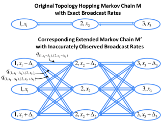
Figure 2: An example of the original three-state topology hopping Markov chain and the extended Markov chain. M is the original topology hopping Markov chain with accurate broadcast rates. M’ is the corresponding extended Markov chain with inaccurate broadcast rate observations. For each configuration $f\in\{1,2,3\}$, the observed broadcast rate takes values $x_{f}-\Delta_{f}$, $x_{f}$, $x_{f}+\Delta_{f}$ with probability $\eta_{-1,f},\eta_{0,f}$ and $\eta_{1,f}$ respectively. The transition rates are assigned according to (32) and (33).

The extended Markov chain has a unique stationary distribution since it is irreducible and only has a finite number of states. We can study the impact of inaccurate broadcast rates by comparing the stationary configuration distribution of the new Markov chain and that of the original topology hopping Markov chain.

We denote the stationary distribution of the states in the new Markov chain by

$$\boldsymbol{\tilde{p}}\triangleq[\tilde{p}_{f,x_{f}+\frac{j}{n_{f}}\Delta_{f}},j\in\{-n_{f},\ldots,n_{f}\},f\in\mathcal{F}].$$ (34)

We also denote $\boldsymbol{\bar{p}}:[\bar{p}_{f}(\boldsymbol{x}),f\in\mathcal{F}]$ as the stationary distribution of the configurations in the extended Markov chain. Given a configuration $f\in\mathcal{F}$, there are $2n_{f}+1$ states associated with $f$ in the extended Markov chain. We have

$$\bar{p}_{f}(\boldsymbol{x})=\sum_{j\in\{-n_{f},\ldots,n_{f}\}}\tilde{p}_{f,x_{f}+\frac{j}{n_{f}}\Delta_{f}},\forall f\in\mathcal{F}.$$ (35)

Recall that the stationary distribution of the configurations for the original topology hopping Markov chain is $\boldsymbol{p^{*}}:[p_{f}^{*}(\boldsymbol{x}),f\in\mathcal{F}]$. We use the total variance distance [36] to quantify the difference between $\boldsymbol{p^{*}}$ and $\boldsymbol{\bar{p}}$, as

$$d_{TV}(\boldsymbol{p^{*}},\boldsymbol{\bar{p}})\triangleq\frac{1}{2}\sum\limits_{f\in\mathcal{F}}|p_{f}^{*}-\bar{p}_{f}|.$$ (36)

We have the following result:

Theorem 3

Let $\Delta_{\max}=\max_{f\in\mathcal{F}}\Delta_{f}$, and $x_{\max}=\max_{f\in\mathcal{F}}x_{f}$. The $d_{TV}(\boldsymbol{p^{*}},\boldsymbol{\bar{p}})$ are bounded as follows:

$$0\leq d_{TV}(\boldsymbol{p^{*}},\boldsymbol{\bar{p}})\leq 1-\exp\left(-2\beta\Delta_{\max}\right).$$ (37)

Further, the optimality gap in broadcast rates $|\boldsymbol{p^{*}}\boldsymbol{x}^{T}-\boldsymbol{\bar{p}}\boldsymbol{x}^{T}|$ is bounded as below:

$$|\boldsymbol{p^{*}}\boldsymbol{x}^{T}-\boldsymbol{\bar{p}}\boldsymbol{x}^{T}|\leq 2x_{\max}(1-\exp(-2\beta\Delta_{\max})).$$ (38)

The proof is relegated to Appendix-C.

Remarks: a) The upper bound on $d_{TV}(\boldsymbol{p^{*}},\boldsymbol{\bar{p}})$ shown in (37) is general, as it is independent of the number of configurations $|\mathcal{F}|$, the values of $n_{f}$, and the distributions of inaccurate observed rates $\eta_{j,f}\;\left(-n_{f}\leq j\leq n_{f},f\in\mathcal{F}\right)$. b) The upper bound on $d_{TV}(\boldsymbol{p^{*}},\boldsymbol{\bar{p}})$ shown in (37) decreases exponentially with the worst inaccuracy bound $\Delta_{\max}$ decreasing. c) It would be interesting to explore a tighter upper bound on $d_{TV}(\boldsymbol{p^{*}},\boldsymbol{\bar{p}})$ than the one in (37).

VI Performance Evaluation

We implement a packet-level simulator to our proposed solutions and use this simulator to evaluate the performance of our solutions.

VI-A Settings

In our simulations, time is chopped into slots of equal length, and we adopt three different settings. In Setting I, we set the total number of nodes to be $100$, and assign the node upload capacities randomly according to the distribution in Table II, which is obtained from the uplink bandwidth statistics of Internet hosts [37]. We set the source’s upload capacity to be $768$ kbps; with this upload capacity, source is not the broadcast bottleneck [1, 3].

Setting II is the same as Setting I, except we set the total number of nodes to be $10$.

In Setting III, there are $4$ different peering configurations as shown in Fig. 3. Every node has a unit capacity. Under configuration $f_{1}$, $f_{2}$ and $f_{3}$ the maximum broadcast rate is $1$, and under configuration $f_{4}$ the maximum broadcast rate is $0.5$.

When running our network coding based broadcasting algorithm, we set the updating step size of $z$ and $\boldsymbol{\lambda}$ to be $0.1$ and $0.00005$ respectively. These parameters are empirically chosen to obtain smooth algorithm updating and small errors.

In our simulations, we assign node degree bounds in the following two ways. The first is to set identical bound on each node’s node degree. The second is to set degree bound proportional to the node’s upload capacity. This is based on the empirical observations that nodes with high upload capacities usually have more system resource (e.g., memory and CPU power) than nodes with low upload capacities. With more system resource, nodes can maintain more concurrent connections, thus have larger node degree bounds. In our second degree bounds assignment, nodes set their node degree bounds proportional to the ratio between their upload capacities and $64$ kbps. In particular, nodes with $64$ kbps have a degree bound of $2$, and nodes with $128$ kbps have a degree bound of $4$, etc.

We carry out two sets of simulations. First, we evaluate the performance of our distributed broadcasting algorithm under Setting I and II. Second, we evaluate the overall performance when we combine the topology hopping algorithm and the broadcasting algorithm under Setting I and III. In these two sets of simulations, we also compare the performance under the two degree bounds assignments explained in the previous paragraph.

TABLE II: Peer upload capacity distribution

Upload Capacity (kbps)	64	128	256	384	768
Fraction (%)	2.8	14.3	4.3	23.3	55.3

Figure 3: Peering configurations under Setting III. For the ease of illustration, we only allow node $1$ to add or remove neighbors between nodes $2$ and $4$. The rest nodes keep their neighbors fixed.

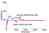
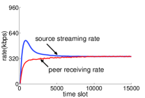
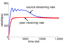
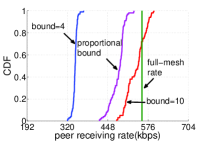
Figure 4: Broadcasting algorithm evaluations. a) The source broadcast rate and average peer receiving rate under Setting II when degree bound is set to $3$; b) The source broadcast rate and average peer receiving rate under Setting I when degree bound is set to $4$; c) The source broadcast rate and average peer receiving rate under Setting I when degree bound is set to 10. d) This figure shows the impact of degree bound on the peer receiving rate under Setting I. The full-mesh rate is the maximum broadcast rate when the node degrees are unbounded [1].

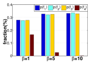
Figure 5: a) Optimal configuration distribution for different values of $\beta$ under Setting III; b) Configuration distribution obtained by our algorithm for different values of $\beta$ under Setting III.

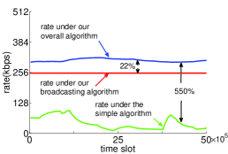
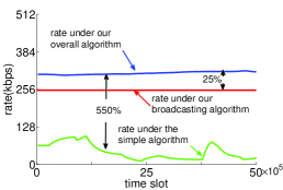
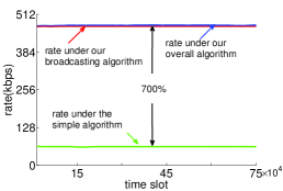
Figure 6: Evaluation of our overall solution which combines the topology hopping algorithm and the broadcasting algorithm. a) The average peer receiving rate when the node degree bound is $3$ and $\beta$ is $20$; b) The average peer receiving rate when the node degree bound is $3$ and $\beta$ is $50$; c) The average peer receiving rate when peer degree bound is proportional to its upload capacity and $\beta$ is $20$. The percentage of average receiving rate improvement of our overall algorithm against our broadcasting algorithm and the simple heuristic algorithm are shown in these three figures. For example, in (a), $22\%$ means that the average receiving rate of our overall algorithm is $1.22$ times of that of our broadcasting algorithm, and $550\%$ means that the average receiving rate of our overall algorithm is $6.5$ times of that of the simple heuristic algorithm.

VI-B Evaluation of the Proposed Broadcasting Algorithm

In this simulation, we evaluate our distributed broadcasting algorithm proposed in Section III. We randomly choose a sub-graph that satisfies the node degree bounds constraints, and run our algorithm over it. We evaluate three aspects of the proposed algorithm: 1) does it converge to optimal broadcast rate as expected from theoretical analysis? 2) How fast does it converge? 3) How would different values of degree bounds affect the maximum broadcast rate? The results are summarized in Fig. 4.

From Fig. 4(a) and Fig. 4(b), we see that our broadcasting algorithm converges. It converges faster in the small size network as shown in Fig. 4(a) than in the large size network as shown in Fig. 4(b). From Fig. 4(d), we also see the converged rate when the node degree bond is $10$ is very close to a theoretical upper bound – the optimal broadcast rate under no degree bounds computed according to [1], [17], [3]. This suggests that our algorithm converges to the optimal broadcast rate.

Under different degree bounds, the optimal broadcast rate varies. Fig. 4(d) shows that the optimal broadcast rate increases when we increase the node degree bounds. We plot the CDF of peer receiving rates (after the broadcasting algorithm converges) for the case where degree bound is $4$, $10$, and proportional to the peer’s upload capacity. It’s seen that when the bound is $10$, the obtained rate is close to the full-mesh rate, which suggests that we do not need a large degree bound to achieve close to the full-mesh rate. The obtained rate is also close to the full-mesh rate when degree bound is proportional to the peer’s upload capacity.

VI-C Evaluation of the Overall Solution

Our overall solution, which combines the Markov chain guided topology hopping algorithm and the back-pressure and network coding based broadcasting algorithm, achieves the near optimal broadcast rate under arbitrary node degree bound and over arbitrary overlay graph. To evaluate its performance, we generate a sub-graph randomly, run our algorithms on every node, and evaluate the achieved broadcast rate.

The topology hopping algorithm runs on top of the broadcasting algorithm. Under given topology, the broadcasting algorithm achieves the optimal broadcast rate. Nodes swap neighbors based on their observed receiving rate, thus changing the topology from time to time. In the simulation, we run the broadcasting algorithm long enough so that it converges before the topology transits according to the Markov chain. This way, the overall algorithm converges to the close-to-optimal broadcast rate.

In all simulations, we compare our overall algorithm with our back-pressure and network coding based broadcasting algorithm to illustrate the benefit of topology hopping, and with a simple heuristic algorithm introduced below to illustrate the benefit of our overall solution. Remind that no existing works solve the problem of streaming-rate maximization under general node degree bounds and over arbitrary topology we studied in this paper.

The simple heuristic algorithm we compare our overall algorithm against is also composed of two parts: routing-based broadcasting algorithm and random topology hopping algorithm. In routing-based broadcasting algorithm, each peer evenly allocates its upload capacity to its neighbors. Given the topology and capacity allocation, a centralized routing strategy (e.g. spanning trees based solution) is used to achieve the best broadcast rate the system can support. Similarly, the random topology hopping algorithm runs on the top of the broadcasting algorithm. Every peer maintains a timer. When the timer of one peer expires, the peer randomly drops one active neighbor which is exchanging data with it, and then selects one random candidate from its feasible neighbor list and starts to exchange data with it. By doing so, we actually allow nodes running the simple scheme to have a node degree beyond the bounds. This relaxation gives the simple scheme more degree of freedom to optimize its performance. Overall, the topology changes randomly on the top under which peers use routing to exchange streaming data.

Our first observation is that our overall scheme converges to the solution that theory predicts. We carry out simulations under Setting III. Under this setting the optimal broadcast rate is $1$. The optimal configuration solution to problem $\mathbf{MRC-\beta}$ is calculated and shown in Fig. 5 for different values of $\beta$. We run the overall scheme for this specific case and show the empirical configuration distribution in Fig. 5. Comparing the distributions in Fig. 5 and Fig. 5, we can see that the distribution obtained by our overall solution is very close to the optimal one. We also calculate the achieved broadcast rate under different values of $\beta$. For $\beta=1,5$ and $10$, the broadcast rate is $0.917$, $0.987$, and $0.998$ respectively. We see that with large $\beta$, the achieved broadcast rate is close to the optimal value $1$, as predicted by our analysis in Section IV.

Next, we evaluate our overall solution under Setting I. In Fig. 6 and Fig. 6, the broadcast rates obtained are $305$ kbps and $312$ kbps respectively. They are about $22\%$ and $25\%$ higher respectively than the broadcast rate $250$ kbps achieved by running the broadcasting algorithm over a randomly chosen topology. This demonstrates the advantage of performing topology hopping to optimize the configuration, as compared to only randomly choosing topology.

By setting node degree bounds proportional to peers’ upload capacity, nodes with higher upload capacity maintain more connections. From Fig. 6, we observe that this flexibility offers a broadcast rate of $475$ kbps. Although the additional gain of topology hopping is small under the specific P2P simulation settings (e.g., node uplink capacity distribution), we remark that our topology-hopping based algorithm is theoretically guaranteed to achieve close-to-optimal streaming rate under arbitrary node degree bounds and P2P settings, while the broadcasting algorithm with random topology selection has no performance guarantee. Moreover, in practical P2P streaming systems, the node degree bounds are typically small. For example, in PPLive, the node degree bounds are 15-20 [15], while the size of the system (i.e., total number of peers that are simultaneously watching the same channel) is usually hundreds of thousands. Thus, we suspect we can see substantial gain of topology hopping if our algorithm is implemented in such system with small node degree bounds, as suggested by our simulation results under small node degree bounds.

From Fig. 6, Fig. 6 and Fig. 6, we observe that the average receiving rate of our overall algorithm is about 5.5-7 times higher than that of the simple algorithm respectively. And also we can see from Fig. 6 and Fig. 6, our algorithm can achieve smoother streaming rate than the simple algorithm because our algorithm optimizes the topology hopping and stays in the optimal topology while the simple algorithm hops among topologies randomly and arbitrarily.

VII Discussions and Future Work

In this paper, we propose a distributed solution to achieve a near-optimal broadcast rate under arbitrary node degree bounds, and over arbitrary overlay graph. Our solution is distributed and consists of two algorithms that can be of independent interests. The first is a distributed broadcasting algorithm that optimizes the broadcast rate given a P2P topology. It is derived from a network coding based problem formulation and utilizes back-pressure arguments. It can be considered as the extension of the algorithm in [30] from link-capacity-limited underlay networks to node-capacity-limited overlay networks. The second algorithm is a Markov chain guided hopping algorithm that optimizes the topology, inspired by the Markov Approximation framework introduced in [20].

Assuming the underlying broadcasting algorithm converges instantaneously, the topology hopping algorithm converges to the optimal configuration distribution. When the broadcasting algorithm does not converge fast enough, the topology hopping Markov chain transits based on inaccurate observations of the maximum broadcast rates associated with the configurations. We show that the topology hopping algorithm still converges, but to a sub-optimal configuration distribution. We characterize an upper bound on the total variance distance between the optimal and sub-optimal configuration distributions, as well as an upper bound on the gap between the achieved and the optimal broadcast rates. We show that both bounds decreases exponentially as the bound on inaccuracy decreases.

Using uplink bandwidth statistics of Internet hosts, our simulations validate the effectiveness of the proposed solutions, and demonstrate the advantage of allowing node degree bounds to scale linearly with their upload capacities.

In the scenarios where network coding is not allowed, we can formulate the broadcasting problem in Subsection III-B as a linear program to construct a feasible node capacity allocation so that the sum of rate of all spanning trees is maximized [15], which is solvable by centralized LP algorithms. Then we can design the overall algorithm in the following way. The overall algorithm is also composed of two separate algorithms: the spanning tree based broadcasting algorithm and the Markov chain guided hopping algorithm. The topology hopping algorithm is same as the one in Section IV which runs on the top of the broadcasting algorithm and guides the topology hopping. Compared to our distributed overall algorithm when network coding is applied, this algorithm is centralized making it unsuited for use in a dynamically changing systems.

Two interesting future directions are as follows. First, the convergence rate of our solution is determined by the mixing time of the topology-hopping Markov chain, which can be substantial for large P2P systems. It is thus of great interest to explore the design of topology-hopping Markov chains that mix fast and at the same time allows distributed implementation. Second, while our algorithms adapt well to peer dynamics, our theoretical analysis is for static scenarios. How to extend the analysis to dynamic scenarios such as those observed in practical P2P systems [38] is another interesting future direction.

Appendix

-A Proof of Theorem 1

We use the following Lyapunov function

$$V(z,\boldsymbol{\lambda},\boldsymbol{\theta})= \frac{1}{2\alpha}(z-z^{*})^{2}+\frac{1}{2}\sum_{v\in V}\sum_{d\in R}\frac{1}{k_{v,d}}(\lambda_{v,d}-\lambda_{v,d}^{*})^{2},$$

where $z^{*},\>\boldsymbol{\lambda}^{*}$ are the saddle points of (9).

By differentiating the Lyapunov function with respect to time we get

$$\dot{V}(z,\boldsymbol{\lambda})$$

$$= (z-z^{*})\left[U^{{}^{\prime}}(z)-\sum_{d\in R}\lambda_{s,d}\right]_{z}^{+}$$

$$+\sum_{v\in V}\sum_{d\in R}(\lambda_{v,d}-\lambda_{v,d}^{*})\left[\sum_{u\in in(v)}f_{uv}^{d}+z\mathbf{1}_{v=s}-\sum_{u\in out(v)}f_{vu}^{d}\right]_{\lambda_{v,d}}^{+}$$

$$\leq (z-z^{*})\left[U^{{}^{\prime}}(z)-\sum_{d\in R}\lambda_{s,d}\right]$$

$$+\sum_{v\in V}\sum_{d\in R}(\lambda_{v,d}-\lambda_{v,d}^{*})\left[\sum_{u\in in(v)}f_{uv}^{d}+z\mathbf{1}_{v=s}-\sum_{u\in out(v)}f_{vu}^{d}\right].$$ (39)

KKT conditions for $z^{*},\boldsymbol{\lambda}^{*}$ are shown as follows

$$U^{{}^{\prime}}(z^{*})-\sum_{d\in R}\lambda_{s,d}^{*}=0$$ (40)

and

$$\lambda_{v,d}^{*}\left[\sum_{u\in in(v)}(f_{uv}^{d})^{*}+z^{*}\mathbf{1}_{v=s}-\sum_{u\in out(v)}(f_{vu}^{d})^{*}\right]=0,\>v\in V,d\in R,$$ (41)

where $\boldsymbol{f}^{*}$is the optimal solution of $\mathbf{MP}$.

From equation (40), we obtain

$$U^{{}^{\prime}}(z^{*})=\sum_{d\in R}\lambda_{s,d}^{*}.$$ (42)

By using the above equation(42), we can transform the terms in the inequality (39) as follows

$$(z-z^{*})\left[U^{{}^{\prime}}(z)-\sum_{d\in R}\lambda_{s,d}\right]$$

$$= (z-z^{*})\left(U^{{}^{\prime}}(z)-U^{{}^{\prime}}(z^{*})\right)+(z-z^{*})\left[\sum_{d\in R}\lambda_{s,d}^{*}-\sum_{d\in R}\lambda_{s,d}\right]$$ (43)

and

$$\sum_{v\in V}\sum_{d\in R}(\lambda_{v,d}-\lambda_{v,d}^{*})\left[\sum_{u\in in(v)}f_{uv}^{d}+z\mathbf{1}_{v=s}-\sum_{u\in out(v)}f_{vu}^{d}\right]$$

$$= \sum_{v\in V}\sum_{d\in R}(\lambda_{v,d}-\lambda_{v,d}^{*})\left[\sum_{u\in in(v)}f_{uv}^{d}+z^{*}\mathbf{1}_{v=s}-\sum_{u\in out(v)}f_{vu}^{d}\right]$$

$$+(z-z^{*})\sum_{d\in R}(\lambda_{s,d}-\lambda_{s,d}^{*}).$$ (44)

We use the above two equations (43) and (44) to substitute the corresponding terms in the inequality (39) and then get

$$\dot{V}(z,\boldsymbol{\lambda})$$

$$\leq (z-z^{*})\left(U^{{}^{\prime}}(z)-U^{{}^{\prime}}(z^{*})\right)$$

$$+\sum_{v\in V}\sum_{d\in R}(\lambda_{v,d}-\lambda_{v,d}^{*})\left[\sum_{u\in in(v)}f_{uv}^{d}+z^{*}\mathbf{1}_{v=s}-\sum_{u\in out(v)}f_{vu}^{d}\right]$$

$$= (z-z^{*})\left(U^{{}^{\prime}}(z)-U^{{}^{\prime}}(z^{*})\right)$$ (45)

$$+\sum_{v\in V}\sum_{d\in R}\lambda_{v,d}\left[\sum_{u\in in(v)}f_{uv}^{d}+z^{*}\mathbf{1}_{v=s}-\sum_{u\in out(v)}f_{vu}^{d}\right]$$ (46)

$$+\sum_{v\in V}\sum_{d\in R}\lambda_{v,d}^{*}\left[\sum_{u\in out(v)}f_{vu}^{d}-\sum_{u\in in(v)}f_{uv}^{d}-z^{*}\mathbf{1}_{v=s}\right].$$ (47)

Next we check the value of (45), (46), (47) respectively. First, the strict concavity of $U(\cdot)$ implies

$$(z-z^{*})\left(U^{{}^{\prime}}(z)-U^{{}^{\prime}}(z^{*})\right)\leq 0.$$ (48)

Since $z^{*},\boldsymbol{\lambda}^{*}$ are optimal solutions, they should satisfy the constraints of the problem $\mathbf{MP}$. So we have

$$\sum_{u\in in(v)}(f_{uv}^{d})^{*}+z^{*}\mathbf{1}_{v=s}\leq\sum_{u\in out(v)}(f_{vu}^{d})^{*}\>v\in V,d\in R.$$

Therefore,

$$\sum_{v\in V}\sum_{d\in R}\lambda_{v,d}\left[\sum_{u\in in(v)}f_{uv}^{d}+z^{*}\mathbf{1}_{v=s}-\sum_{u\in out(v)}f_{vu}^{d}\right]$$

$$\leq \sum_{v\in V}\sum_{d\in R}\lambda_{v,d}\left[\sum_{u\in in(v)}f_{uv}^{d}-\sum_{u\in out(v)}f_{vu}^{d}+\sum_{u\in out(v)}(f_{vu}^{d})^{*}-\sum_{u\in in(v)}(f_{uv}^{d})^{*}\right]$$

$$= \sum_{v\in V}\sum_{d\in R}\lambda_{v,d}\left[\sum_{u\in in(v)}f_{uv}^{d}-\sum_{u\in out(v)}f_{vu}^{d}\right]$$

$$-\sum_{v\in V}\sum_{d\in R}\lambda_{v,d}\left[\sum_{u\in in(v)}(f_{uv}^{d})^{*}-\sum_{u\in out(v)}(f_{vu}^{d})^{*}\right].$$

Note that $\boldsymbol{f}$ is the solution of the following problem

$$\max \sum_{v\in V}\sum_{d\in R}\lambda_{v,d}\left[\sum_{u\in out(v)}f_{vu}^{d}-\sum_{u\in in(v)}f_{uv}^{d}\right]$$

s.t. $$\eqref{eq:MPC2}-\eqref{eq:MPC3},$$

which is equivalent to $\mathbf{SSP}$. Since $\boldsymbol{f}^{*}$is also feasible, for (46) we have

$$\sum_{v\in V}\sum_{d\in R}\lambda_{v,d}\left[\sum_{u\in in(v)}f_{uv}^{d}+z^{*}\mathbf{1}_{v=s}-\sum_{u\in out(v)}f_{vu}^{d}\right]$$

$$\leq \sum_{v\in V}\sum_{d\in R}\lambda_{v,d}\left[\sum_{u\in in(v)}f_{uv}^{d}-\sum_{u\in out(v)}f_{vu}^{d}\right]$$

$$-\sum_{v\in V}\sum_{d\in R}\lambda_{v,d}\left[\sum_{u\in in(v)}(f_{uv}^{d})^{*}-\sum_{u\in out(v)}(f_{vu}^{d})^{*}\right]$$

$$\leq 0.$$

Now we focus on the term(47). According to (41), the following equality holds.

$$\sum_{v\in V}\sum_{d\in R}\lambda_{v,d}^{*}\left[\sum_{u\in out(v)}f_{vu}^{d}-\sum_{u\in in(v)}f_{uv}^{d}-z^{*}\mathbf{1}_{v=s}\right]$$

$$= \sum_{v\in V}\sum_{d\in R}\lambda_{v,d}^{*}\left[\sum_{u\in out(v)}f_{uv}^{d}-\sum_{u\in in(v)}f_{vu}^{d}+\sum_{u\in in(v)}(f_{vu}^{d})^{*}-\sum_{u\in out(v)}(f_{uv}^{d})^{*}\right]$$

$$= \sum_{v\in V}\sum_{d\in R}\lambda_{v,d}^{*}\left[\sum_{u\in out(v)}f_{uv}^{d}-\sum_{u\in in(v)}f_{vu}^{d}\right]$$

$$-\sum_{v\in V}\sum_{d\in R}\lambda_{v,d}^{*}\left[\sum_{u\in out(v)}(f_{uv}^{d})^{*}-\sum_{u\in in(v)}(f_{vu}^{d})^{*}\right].$$

Note that $\boldsymbol{f}^{*}$ is the solution of the following problem

$$\max \sum_{v\in V}\sum_{d\in R}\lambda_{v,d}^{*}\left[\sum_{u\in out(v)}f_{vu}^{d}-\sum_{u\in in(v)}f_{uv}^{d}\right]$$

s.t. $$\eqref{eq:MPC2}-\eqref{eq:MPC3}.$$

So,

$$\sum_{v\in V}\sum_{d\in R}\lambda_{v,d}^{*}\left[\sum_{u\in out(v)}f_{vu}^{d}-\sum_{u\in in(v)}f_{uv}^{d}-z^{*}\mathbf{1}_{v=s}\right]$$

$$= \sum_{v\in V}\sum_{d\in R}\lambda_{v,d}^{*}\left[\sum_{u\in out(v)}f_{uv}^{d}-\sum_{u\in in(v)}f_{vu}^{d}\right]$$

$$-\sum_{v\in V}\sum_{d\in R}\lambda_{v,d}^{*}\left[\sum_{u\in out(v)}(f_{uv}^{d})^{*}-\sum_{u\in in(v)}(f_{vu}^{d})^{*}\right]$$

$$\leq 0.$$

Overall, we get

$$\dot{V}(z,\boldsymbol{\lambda})$$

$$\leq (z-z^{*})\left(U^{{}^{\prime}}(z)-U^{{}^{\prime}}(z^{*})\right)$$

$$+\sum_{v\in V}\sum_{d\in R}\lambda_{v,d}\left[\sum_{u\in in(v)}f_{uv}^{d}+z^{*}\mathbf{1}_{v=s}-\sum_{u\in out(v)}f_{vu}^{d}\right]$$

$$+\sum_{v\in V}\sum_{d\in R}\lambda_{v,d}^{*}\left[\sum_{u\in out(v)}f_{vu}^{d}-\sum_{u\in in(v)}f_{uv}^{d}-z^{*}\mathbf{1}_{v=s}\right]$$

$$\leq 0.$$

Let $\mathcal{E}\triangleq\{(z,\boldsymbol{\lambda})|\,\dot{V}(z,\boldsymbol{\lambda})=0\}$ and $\mathcal{G}\triangleq\{(z,\boldsymbol{\lambda})|\,\eqref{eq:bound1}=0,\eqref{eq:bound2}=0,\eqref{eq:bound3}=0\}$. Since $\dot{V}(z,\boldsymbol{\lambda})\leq\eqref{eq:bound1}+\eqref{eq:bound2}+\eqref{eq:bound3}$ and $\eqref{eq:bound1}\leq 0,\eqref{eq:bound2}\leq 0,\eqref{eq:bound3}\leq 0,$ we have $\mathcal{E}\subset\mathcal{G}$. Let $\mathcal{M}$ be the largest invariant set in $\mathcal{E}$. By LaSalle’s invariance principle $(z(t),\boldsymbol{\lambda}(t))$ converges to the set $\mathcal{M}$ as $t\rightarrow\infty$. Since $\mathcal{M}\subset\mathcal{E}\subset\mathcal{G}$, as $t\rightarrow\infty$ $(z(t),\boldsymbol{\lambda}(t))$ satisfies

$$z(t)=z^{*}$$ (49)

and

$$\sum_{v\in V}\sum_{d\in R}\left(\lambda_{v,d}(t)-\lambda_{v,d}^{*}(t)\right)\left[\sum_{u\in in(v)}f_{uv}^{d}(t)+z^{*}\mathbf{1}_{v=s}-\sum_{u\in out(v)}f_{vu}^{d}(t)\right]=0.$$ (50)

Further, in $\mathcal{M}$, $\sum_{d\in R}\lambda_{s,d}(t)=U^{{}^{\prime}}(z^{*})$. To see this, if this is not satisfied, then by (20) we can see $z(t)$ will not stay in $z^{*}$, which is contradicted with (49). This concludes the proof.

-B Proof of Proposition 1

By two conditions for state space structure of Markov chain, we know that all configurations can reach each other within a finite number of transitions, thus the constructed Markov chain is irreducible. Further, it is a finite state ergodic Markov chain with a unique stationary distribution. We now show that the stationary distribution of the constructed Markov chain is indeed (27).

Now we verify that under the implementation, the state transition rate from $f$ to $f^{{}^{\prime}}$ satisfies (29).

In our Markov chain design, we only allow direct transitions between two configurations if such transitions correspond to a single node adding a new neighbor or removing a neighbor, i.e., $|\mathcal{N}_{f}\backslash\mathcal{N}_{f^{\prime}}|=1$ or $|\mathcal{N}_{f^{\prime}}\backslash\mathcal{N}_{f}|=1$. We consider these two scenarios separately in the following.

Let $f\rightarrow f^{{}^{\prime}}$ denote the event that when the timer expires the process will enter state $f^{{}^{\prime}}$ after leaving the current state $f$. The probability of this event is denoted by $\Pr(f\rightarrow f^{{}^{\prime}})$.

When $|\mathcal{N}_{f}\backslash\mathcal{N}_{f^{\prime}}|=1$, assuming $\mathcal{N}_{f}\backslash\mathcal{N}_{f^{\prime}}=(v,u)$, the event $f\rightarrow f^{{}^{\prime}}$ can be divided into two disjoint events: the event that node $v$’s timer expires, then node $v$ selects node $u$ to remove and remove it from its in-use neighbor set and the event that node $u$’s timer expires, then node $u$ selects node $v$ to remove and remove it from its in-use neighbor set. Denote these two events by $f\,\underrightarrow{v-u}\,f^{{}^{\prime}}$ and $f\,\underrightarrow{u-v}\,f^{{}^{\prime}}$ . Let $v-u$ be the event that node $v$ selects node $u$ and removes it from its in-use neighbor set and $u-v$ be the event that node $u$ selects node $v$ and removes it from its in-use neighbor set. Now we calculate the probability of $f\,\underrightarrow{v-u}\,f^{{}^{\prime}}$ and $f\,\underrightarrow{u-v}\,f^{{}^{\prime}}$ respectively.

$$\Pr(f\,\underrightarrow{v-u}\,f^{{}^{\prime}})$$

$$= \Pr(v-u|v\mbox{'s timer expires})\Pr(v\mbox{'s timer expires})$$

$$= \frac{|N_{v,f}|}{|N_{v}|}\cdot\frac{1}{|N_{v,f}|}\cdot\frac{\exp(\beta x_{f^{{}^{\prime}}})}{\exp(\beta x_{f})+\exp(\beta x_{f^{{}^{\prime}}})}\cdot\frac{\frac{|N_{v}|}{2\exp(\tau)}}{\sum_{w\in V}\frac{|N_{w}|}{2\exp(\tau)}}$$

$$= \frac{1}{\sum_{v\in V}|N_{v}|}\cdot\frac{\exp(\beta x_{f^{{}^{\prime}}})}{\exp(\beta x_{f})+\exp(\beta x_{f^{{}^{\prime}}})}$$ (51)

and

$$\Pr(f\,\underrightarrow{u-v}\,f^{{}^{\prime}})$$

$$= \Pr(u-v|u\mbox{'s timer expires})\Pr(u\mbox{'s timer expires})$$

$$= \frac{|N_{u,f}|}{|N_{u}|}\cdot\frac{1}{|N_{u,f}|}\cdot\frac{\exp(\beta x_{f^{{}^{\prime}}})}{\exp(\beta x_{f})+\exp(\beta x_{f^{{}^{\prime}}})}\cdot\frac{\frac{|N_{u}|}{2\exp(\tau)}}{\sum_{w\in V}\frac{|N_{w}|}{2\exp(\tau)}}$$

$$= \frac{1}{\sum_{v\in V}|N_{v}|}\cdot\frac{\exp(\beta x_{f^{{}^{\prime}}})}{\exp(\beta x_{f})+\exp(\beta x_{f^{{}^{\prime}}})}.$$ (52)

Therefore, we have

$$\Pr(f\rightarrow f^{{}^{\prime}})$$

$$= \Pr(f\,\underrightarrow{v-u}\,f^{{}^{\prime}})+\Pr(f\,\underrightarrow{u-v}\,f^{{}^{\prime}})$$

$$= \frac{2}{\sum_{v\in V}|N_{v}|}\cdot\frac{\exp(\beta x_{f^{{}^{\prime}}})}{\exp(\beta x_{f})+\exp(\beta x_{f^{{}^{\prime}}})}.$$ (53)

When $|\mathcal{N}_{f^{\prime}}\backslash\mathcal{N}_{f}|=1$, assuming $\mathcal{N}_{f^{\prime}}\backslash\mathcal{N}_{f}=(v,u)$, similarly we divide $f\rightarrow f^{{}^{\prime}}$ into two disjoint events $f\,\underrightarrow{v+u}\,f^{{}^{\prime}}$ and $f\,\underrightarrow{u+v}\,f^{{}^{\prime}}$. $f\,\underrightarrow{v+u}\,f^{{}^{\prime}}$ denotes the event that node $v$’s timer expires, then node $v$ selects node $u$ to add and add it in its in-use neighbor set. $f\,\underrightarrow{u+v}\,f^{{}^{\prime}}$ denotes the event that node $u$’s timer expires, then node $u$ selects node $v$ to add and add it in its in-use neighbor set. Let $v+u$ be the event that node $v$ selects node $u$ and adds it as one in-use neighbor and $u+v$ be the event that node $u$ selects node $v$ and adds it as one in-use neighbor. Then we have

$$\Pr(f\,\underrightarrow{v+u}\,f^{{}^{\prime}})$$

$$= \Pr(v+u|v\mbox{'s timer expires})\Pr(v\mbox{'s timer expires})$$

$$= \frac{|N_{v}|-|N_{v,f}|}{|N_{v}|}\cdot\frac{1}{|N_{v}|-|N_{v,f}|}\cdot\frac{\exp(\beta x_{f^{{}^{\prime}}})}{\exp(\beta x_{f})+\exp(\beta x_{f^{{}^{\prime}}})}\cdot\frac{\frac{|N_{v}|}{2\exp(\tau)}}{\sum_{w\in V}\frac{|N_{w}|}{2\exp(\tau)}}$$

$$= \frac{1}{\sum_{v\in V}|N_{v}|}\cdot\frac{\exp(\beta x_{f^{{}^{\prime}}})}{\exp(\beta x_{f})+\exp(\beta x_{f^{{}^{\prime}}})}$$ (54)

and

$$\Pr(f\,\underrightarrow{u+v}\,f^{{}^{\prime}})$$

$$= \Pr(u+v|u\mbox{'s timer expires})\Pr(u\mbox{'s timer expires})$$

$$= \frac{|N_{u}|-|N_{u,f}|}{|N_{u}|}\cdot\frac{1}{|N_{u}|-|N_{u,f}|}\cdot\frac{\exp(\beta x_{f^{{}^{\prime}}})}{\exp(\beta x_{f})+\exp(\beta x_{f^{{}^{\prime}}})}\cdot\frac{\frac{|N_{u}|}{2\exp(\tau)}}{\sum_{w\in V}\frac{|N_{w}|}{2\exp(\tau)}}$$

$$= \frac{1}{\sum_{v\in V}|N_{v}|}\cdot\frac{\exp(\beta x_{f^{{}^{\prime}}})}{\exp(\beta x_{f})+\exp(\beta x_{f^{{}^{\prime}}})}.$$ (55)

Therefore, we have

$$\Pr(f\rightarrow f^{{}^{\prime}})$$

$$= \Pr(f\,\underrightarrow{v+u}\,f^{{}^{\prime}})+\Pr(f\,\underrightarrow{u+v}\,f^{{}^{\prime}})$$

$$= \frac{2}{\sum_{v\in V}|N_{v}|}\cdot\frac{\exp(\beta x_{f^{{}^{\prime}}})}{\exp(\beta x_{f})+\exp(\beta x_{f^{{}^{\prime}}})}.$$ (56)

In our implementation, under configuration $f$, peer $v$ counts down with rate $\frac{|N_{v}|}{2}\exp^{-1}(\tau)$. Therefore, the rate of leaving the state $f$ is $\sum_{v\in{V}}\frac{|N_{v}|}{2}\exp^{-1}(\tau)$. With the probability $\Pr(f\rightarrow f^{{}^{\prime}})$, the process jumps to state $f^{{}^{\prime}}$ when leaving state $f$. So, the transition rate from state $f$ to $f^{{}^{\prime}}$ is

$$q_{f,f^{\prime}}=\frac{2}{\sum_{v\in V}|N_{v}|}\cdot\frac{\exp(\beta\cdot x_{f^{{}^{\prime}}})}{\exp(\beta\cdot x_{f})+\exp(\beta\cdot x_{f^{{}^{\prime}}})}$$

$$\times\sum_{v\in V}\frac{|N_{v}|}{2}\exp^{-1}(\tau)$$

$$=\exp^{-1}(\tau)\frac{\exp(\beta\cdot x_{f^{{}^{\prime}}})}{\exp(\beta\cdot x_{f})+\exp(\beta\cdot x_{f^{{}^{\prime}}})}.$$ (57)

With (27), we see that $p_{f}^{*}(\boldsymbol{x})\cdot q_{f,f^{\prime}}=p_{f^{\prime}}^{*}(\boldsymbol{x})\cdot q_{f^{\prime},f},\forall f,f^{\prime}\in\mathcal{F}$, i.e., the detailed balance equations hold. Thus the constructed Markov chain is time-reversible and its stationary distribution is indeed (27) according to Theorem 1.3 and Theorem 1.14 in [39].

-C Proof of Theorem 3

We denote $M$ as the original topology hopping Markov chain with exact broadcast rates, and $M^{\prime}$ as the corresponding extended Markov chain with inaccurately observed broadcast rates. For the convenience of expression, for all $f\in\mathcal{F},j\in\{-n_{f},\ldots,n_{f}\}$, we use $f_{j}$ to represent the state $(f,x_{f}+\frac{j}{n_{f}}\Delta_{f})$ in the extended Markov chain $M^{\prime}$, and $\eta_{f_{j}}$ to represent distribution of inaccurate observed rates $\eta_{j,f}$.

Therefore, given direct transitions between configuration $f$ and $f^{\prime}$ in the original topology hopping Markov chain $M$, there are direct transitions between states $f_{j}$ and $f^{\prime}_{k}$ ($\forall j\in\{-n_{f},\ldots,n_{f}\},k\in\{-n_{f^{\prime}},\ldots,n_{f^{\prime}}\}$) in the extended Markov chain $M^{\prime}$. Following (32) and (33), we have the corresponding transition rates

$$q_{f_{j},f^{\prime}_{k}}=\frac{\eta_{f^{\prime}_{k}}}{\exp(\tau)}\cdot\frac{\exp(\beta(x_{f^{\prime}}+\frac{k}{n_{f^{\prime}}}\Delta_{f^{\prime}}))}{\exp(\beta(x_{f^{\prime}}+\frac{k}{n_{f^{\prime}}}\Delta_{f^{\prime}}))+\exp(\beta(x_{f}+\frac{j}{n_{f}}\Delta_{f}))}$$ (58)

and

$$q_{f^{\prime}_{k},f_{j}}=\frac{\eta_{f_{j}}}{\exp(\tau)}\cdot\frac{\exp(\beta(x_{f}+\frac{j}{n_{f}}\Delta_{f}))}{\exp(\beta(x_{f}+\frac{j}{n_{f}}\Delta_{f}))+\exp(\beta(x_{f^{\prime}}+\frac{k}{n_{f^{\prime}}}\Delta_{f^{\prime}}))},$$ (59)

where $\sum_{j=-n_{f}}^{n_{f}}\eta_{f_{j}}=1$ and $\sum_{k=-n_{f^{\prime}}}^{n_{f^{\prime}}}\eta_{f^{\prime}_{k}}=1$.

Now we compute the stationary distribution of states for the extended Markov chain $M^{\prime}$. By detailed balance equation, we have

$$p_{f_{j}}q_{f_{j},f^{\prime}_{k}}=p_{f^{\prime}_{k}}q_{f^{\prime}_{k},f_{j}},\forall j\in\{-n_{f},\ldots,n_{f}\},k\in\{-n_{f^{\prime}},\ldots,n_{f^{\prime}}\}.$$ (60)

Then we have

$$p_{f_{j}}\cdot\frac{1}{\eta_{f_{j}}\cdot\exp(\beta(x_{f}+\frac{j}{n_{f}}\Delta_{f}))}=p_{f^{\prime}_{k}}\cdot\frac{1}{\eta_{f^{\prime}_{k}}\cdot\exp(\beta(x_{f^{\prime}}+\frac{k}{n_{f^{\prime}}}\Delta_{f^{\prime}}))},$$ (61)

$$\forall j\in\{-n_{f},\ldots,n_{f}\},k\in\{-n_{f^{\prime}},\ldots,n_{f^{\prime}}\}.$$

Therefore,

$$\frac{p_{f_{0}}}{\eta_{f_{0}}\cdot\exp(\beta x_{f})}=\frac{p_{f^{\prime}_{0}}}{\eta_{f^{\prime}_{0}}\cdot\exp(\beta x_{f^{\prime}})}$$ (62)

and

$$\frac{p_{f^{\prime}_{k}}}{p_{f^{\prime}_{0}}}=\frac{\eta_{f^{\prime}_{k}}}{\eta_{f^{\prime}_{0}}}\cdot\exp(\beta\frac{k}{n_{f^{\prime}}}\Delta_{f^{\prime}}),\forall k\in\{-n_{f^{\prime}},\ldots,n_{f^{\prime}}\}.$$ (63)

Consider an arbitrary state $\hat{f}_{0}$ in the extended Markov chain $M^{\prime}$, where $\hat{f}\in\mathcal{F}$ and $\hat{f}\neq f,f^{\prime}$. Since state space of $M^{\prime}$ is connected, we can always find a path to connect $\hat{f}_{0}$ and $f_{0}$ through a series of adjacent states $\tilde{f}(1)_{0},\ldots,\tilde{f}(L)_{0}$, and $f_{0}=\tilde{f}(1)_{0},\tilde{f}(L)_{0}=\hat{f}_{0}$. Therefore,

$$\frac{p_{\hat{f}_{0}}}{p_{f_{0}}}=\prod_{l=1}^{L-1}\frac{p_{\tilde{f}(l+1)_{0}}}{p_{\tilde{f}(l)_{0}}}$$ (64)

and by (62) we have

$$\frac{p_{\tilde{f}(l+1)_{0}}}{\eta_{\tilde{f}(l+1)_{0}}\cdot\exp(\beta x_{\tilde{f}(l+1)})}=\frac{p_{\tilde{f}(l)_{0}}}{\eta_{\tilde{f}(l)_{0}}\cdot\exp(\beta x_{\tilde{f}(l)})}.$$ (65)

Then

$$\frac{p_{\hat{f}_{0}}}{\eta_{\hat{f}_{0}}\cdot\exp(\beta x_{\hat{f}})}=\frac{p_{f_{0}}}{\eta_{f_{0}}\cdot\exp(\beta x_{f})}.$$ (66)

By (63) and (66), we know that $\forall f\in\mathcal{F}$,

$$\frac{p_{f_{0}}}{\eta_{f_{0}}\cdot\exp(\beta x_{f})}\text{ is a constant}$$ (67)

and

$$\frac{p_{f_{j}}}{p_{f_{0}}}=\frac{\eta_{f_{j}}}{\eta_{f_{0}}}\cdot\exp(\beta\frac{j}{n_{f}}\Delta_{f}),\forall j\in\{-n_{f},\ldots,n_{f}\}.$$ (68)

On the other hand, we have

$$\sum\limits_{f\in\mathcal{F}}{\sum\limits_{j=-n_{f}}^{n_{f}}{p_{f_{j}}}}=1.$$ (69)

By (67), (68) and (69), we obtain the stationary distribution of states for the extended Markov chain $M^{\prime}$ as follows:

$$\forall f\in\mathcal{F},j\in\{-n_{f},\ldots,n_{f}\},$$

$$\tilde{p}_{f_{j}}=\frac{\eta_{f_{j}}\cdot\exp(\beta(x_{f}+\frac{j}{n_{f}}\Delta_{f}))}{\sum\limits_{f^{\prime}\in\mathcal{F}}\sum\limits_{k=-n_{f^{\prime}}}^{n_{f^{\prime}}}\eta_{f^{\prime}_{k}}\cdot\exp(\beta(x_{f^{\prime}}+\frac{k}{n_{f^{\prime}}}\Delta_{f^{\prime}}))}.$$ (70)

The stationary distribution of peer configurations in the extended Markov chain $M^{\prime}$ is the probability distribution of aggregate states $f_{j},j\in\{-n_{f},\ldots,n_{f}\}$, i.e.,

$$\bar{p}_{f}=\sum\limits_{j=-n_{f}}^{n_{f}}\tilde{p}_{f_{j}}.$$ (71)

Let

$$\alpha_{f}\triangleq\sum\limits_{j=-n_{f}}^{n_{f}}\eta_{f_{j}}\cdot\exp(\beta\frac{j}{n_{f}}\Delta_{f}),\forall f\in\mathcal{F}.$$ (72)

Then we have

$$\bar{p}_{f}=\frac{\alpha_{f}\exp(\beta x_{f})}{\sum\limits_{f^{\prime}\in\mathcal{F}}\alpha_{f^{\prime}}\exp(\beta x_{f^{\prime}})},\forall f\in\mathcal{F}.$$ (73)

By (27), we know

$$p^{*}_{f}=\frac{\exp(\beta x_{f})}{\sum\limits_{f^{\prime}\in\mathcal{F}}\exp(\beta x_{f^{\prime}})},\forall f\in\mathcal{F}.$$ (74)

Let

$$\bar{\alpha}\triangleq\frac{\sum\limits_{f^{\prime}\in\mathcal{F}}\alpha_{f^{\prime}}\exp(\beta x_{f^{\prime}})}{\sum\limits_{f^{\prime}\in\mathcal{F}}\exp(\beta x_{f^{\prime}})}.$$ (75)

It is not hard to see that $\frac{p^{*}_{f}}{\bar{p}_{f}}=\frac{\bar{\alpha}}{\alpha_{f}}$, so

$$p^{*}_{f}\geq\bar{p}_{f}\text{ iff }\alpha_{f}\leq\bar{\alpha}.$$ (76)

The total variation distance

$$d_{TV}(\boldsymbol{p^{*}},\boldsymbol{\bar{p}}) =\frac{1}{2}\sum\limits_{f\in\mathcal{F}}|p^{*}_{f}-\bar{p}_{f}|$$ (77)

$$=\sum\limits_{f\in A}(p^{*}_{f}-\bar{p}_{f}),$$ (78)

where $A\triangleq\{f\in\mathcal{F}:p^{*}_{f}\geq\bar{p}_{f}\}$.

By (76), we know $A=\{f\in\mathcal{F}:\alpha_{f}\leq\bar{\alpha}\}\subset\mathcal{F}$.

Therefore, $\forall f\in A$,

$$p^{*}_{f}-\bar{p}_{f} =\frac{\exp(\beta x_{f})}{\sum\limits_{f^{\prime}\in\mathcal{F}}\exp(\beta x_{f^{\prime}})}-\frac{\alpha_{f}\exp(\beta x_{f})}{\sum\limits_{f^{\prime}\in\mathcal{F}}\alpha_{f^{\prime}}\exp(\beta x_{f^{\prime}})}$$ (79)

$$=\frac{\exp(\beta x_{f})}{\sum\limits_{f^{\prime}\in\mathcal{F}}\exp(\beta x_{f^{\prime}})}-\frac{\alpha_{f}\exp(\beta x_{f})}{\bar{\alpha}\sum\limits_{f^{\prime}\in\mathcal{F}}\exp(\beta x_{f^{\prime}})}$$ (80)

$$=\frac{\exp(\beta x_{f})}{\sum\limits_{f^{\prime}\in\mathcal{F}}\exp(\beta x_{f^{\prime}})}[1-\frac{\alpha_{f}}{\bar{\alpha}}].$$ (81)

Since $\sum\limits_{j=-n_{f}}^{n_{f}}\eta_{f_{j}}=1$ and $\forall j\in\{-n_{f},\ldots,n_{f}\}$,

$$\exp(\beta\frac{j}{n_{f}}\Delta_{f})\geq\exp(-\beta\Delta_{f})\geq\exp(-\beta\Delta_{\max})$$ (82)

and

$$\exp(\beta\frac{j}{n_{f}}\Delta_{f})\leq\exp(\beta\Delta_{f})\leq\exp(\beta\Delta_{\max}),$$ (83)

by (72) we know that $\forall f\in\mathcal{F}$

$$\alpha_{f}\geq\sum\limits_{j=-n_{f}}^{n_{f}}\eta_{f_{j}}\cdot\exp(-\beta\Delta_{\max})=\exp(-\beta\Delta_{\max})$$ (84)

and

$$\alpha_{f}\leq\sum\limits_{j=-n_{f}}^{n_{f}}\eta_{f_{j}}\cdot\exp(\beta\Delta_{\max})=\exp(\beta\Delta_{\max}).$$ (85)

Then by (75), we have $\bar{\alpha}\leq\exp(\beta\Delta_{\max})$. Therefore,

$$1-\frac{\alpha_{f}}{\bar{\alpha}}\leq 1-\frac{\exp(-\beta\Delta_{\max})}{\exp(\beta\Delta_{\max})}=1-\exp(-2\beta\Delta_{\max}),\forall f\in A\subset\mathcal{F}.$$ (86)

So by (81), we have $\forall f\in A$,

$$p^{*}_{f}-\bar{p}_{f} =\frac{\exp(\beta x_{f})}{\sum\limits_{f^{\prime}\in\mathcal{F}}\exp(\beta x_{f^{\prime}})}[1-\frac{\alpha_{f}}{\bar{\alpha}}]$$ (87)

$$\leq\frac{\exp(\beta x_{f})}{\sum\limits_{f^{\prime}\in\mathcal{F}}\exp(\beta x_{f^{\prime}})}(1-\exp(-2\beta\Delta_{\max})).$$ (88)

Then,

$$d_{TV}(\boldsymbol{p^{*}},\boldsymbol{\bar{p}}) =\sum\limits_{f\in A}(p^{*}_{f}-\bar{p}_{f})$$ (89)

$$\leq\sum\limits_{f\in A}\frac{\exp(\beta x_{f})}{\sum\limits_{f^{\prime}\in\mathcal{F}}\exp(\beta x_{f^{\prime}})}(1-\exp(-2\beta\Delta_{\max}))$$ (90)

$$\leq\sum\limits_{f\in\mathcal{F}}\frac{\exp(\beta x_{f})}{\sum\limits_{f^{\prime}\in\mathcal{F}}\exp(\beta x_{f^{\prime}})}(1-\exp(-2\beta\Delta_{\max}))$$ (91)

$$=1-\exp(-2\beta\Delta_{\max}).$$ (92)

Therefore,

$$|\boldsymbol{p^{*}}\boldsymbol{x}^{T}-\boldsymbol{\bar{p}}\boldsymbol{x}^{T}| =|\sum\limits_{f\in\mathcal{F}}(p^{*}_{f}-\bar{p}_{f})x_{f}|$$ (93)

$$\leq x_{\max}\sum\limits_{f\in\mathcal{F}}|(p^{*}_{f}-\bar{p}_{f})|$$ (94)

$$=2x_{\max}d_{TV}(\boldsymbol{p^{*}},\boldsymbol{\bar{p}})$$ (95)

$$\leq 2x_{\max}(1-\exp(-2\beta\Delta_{\max})).$$ (96)

This concludes the proof.

References

- [1] J. Li, P. A. Chou, and C. Zhang, “Mutualcast: an efficient mechanism for content distribution in a p2p network,” in Proc. ACM SIGCOMM Asia Workshop, 2005.
- [2] L. Massoulie, A. Twigg, G. Gkantsidis, and P. Rodriguez, “Randomized Decentralized Broadcasting Algorithms,” in Proc. IEEE INFOCOM, 2007.
- [3] R. Kumar, Y. Liu, and K. Ross, “Stochastic fluid theory for p2p streaming systems,” in Proc. IEEE INFOCOM, 2007.
- [4] Y. Cui, Y. Xue, and K. Nahrstedt, “Optimal resource allocation in overlay multicast,” IEEE Trans. Parallel and Distributed Systems, vol. 17, pp. 808–823, 2006.
- [5] S. Sengupta, S. Liu, M. Chen, M. Chiang, J. Li, and P. A. Chou, “Peer-to-peer streaming capacity,” IEEE Trans. Information Theory, vol. 57, pp. 5072–5087, 2011.
- [6] M. Castro, P. Druschel, A. Kermarrec, A. Nandi, A. Rowstron, and A. Singh, “SplitStream: high-bandwidth multicast in cooperative environments,” in Proc. ACM SOSP, 2003.
- [7] V. Padmanabhan and K. Sripanidkulchai, “The case for cooperative networking,” in Proc. IPTPS, 2002.
- [8] D. A. Tran, K. Hua, and T. Do, “ZIGZAG: An efficient peer-to-peer scheme for media streaming,” in Proc. IEEE INFOCOM, 2003.
- [9] N. Magharei and R. Rejaie, “PRIME: Peer-to-peer receiver-driven mesh-based streaming,” IEEE/ACM Trans. Networking, vol. 17, pp. 1052–1065, 2009.
- [10] S. Liu, M. Chen, S. Sengupta, M. Chiang, J. Li, and P. A. Chou, “Peer-to-peer streaming capacity under node degree bound,” in Proc. IEEE ICDCS, 2010.
- [11] C. Feng, B. Li, and B. Li, “Understanding the performance gap between pull-based mesh streaming protocols and fundamental limits,” in Proc. IEEE INFOCOM, 2009.
- [12] L. Abeni, C. Kiraly, and R. L. Cigno, “On the optimal scheduling of streaming applications in unstructured meshes,” in Proc. IFIP Networking, 2009.
- [13] M. Wang and B. Li, “R2: Random Push with Random Network Coding in Live Peer-to-Peer Streaming,” IEEE Journal on Selected Areas in Communications, vol. 25, p. 1655, 2007.
- [14] X. Zhang, J. Liu, B. Li, and T. Yum, “CoolStreaming/DONet: A data-driven overlay network for efficient live media streaming,” in Proc. IEEE INFOCOM, 2005.
- [15] M. Chen, M. Chiang, P. A. Chou, J. Li, S. Liu, and S. Sengupta, “Peer-to-peer streaming capacity: Survey and recent results,” in Proc. Allerton Conference, 2009.
- [16] D. M. Chiu, R. W. Yeung, J. Huang, and B. Fan, “Can network coding help in p2p networks?” in Proc. IEEE NetCod, 2006.
- [17] M. Chen, M. Ponec, S. Sengupta, J. Li, and P. Chou, “Utility maximization in peer-to-peer systems,” in Proc. ACM SIGMETRICS, 2008.
- [18] PPLive. [Online]. Available: http://www.pplive.com
- [19] UUSee. [Online]. Available: http://www.uusee.com
- [20] M. Chen, S. C. Liew, Z. Shao, and C. Kai, “Markov approximation for combinatorial network optimization,” in Proc. IEEE INFOCOM, 2010.
- [21] R. Ahlswede, N. Cai, S.-Y. R. Li, and R. W. Yeung, “Network information flow,” IEEE Trans. Information Theory, pp. 1204–1216, 2000.
- [22] L. Tassiulas and A. Ephremides, “Stability properties of constrained queueing systems and scheduling policies for maximum throughput in multihop radio networks,” IEEE Trans. Automatic Control, vol. 37, pp. 1936–1948, 1992.
- [23] N. McKeown, V. Anantharam, and J. Walrand, “Achieving 100% throughput in an input-queued switch,” in Proc. IEEE INFOCOM, 1996.
- [24] A. Eryilmaz, R. Srikant, and J. Perkins, “Stable scheduling policies for fading wireless channels,” IEEE/ACM Trans. on Networking, vol. 13, pp. 411–424, 2005.
- [25] M. Neely, E. Modiano, and C. Rohrs, “Dynamic power allocation and routing for time-varying wireless networks,” IEEE Journal on Selected Areas in Communications, vol. 23, pp. 89–103, 2005.
- [26] J. Liu, S. Rao, B. Li, and H. Zhang, “Opportunities and challenges of peer-to-peer internet video broadcast,” in Proc. IEEE, 2008.
- [27] Z. Liu, C. Wu, B. Li, and S. Zhao, “Uusee: Large-scale operational on-demand streaming with random network coding,” in Proc. IEEE INFOCOM, 2010.
- [28] X. Hei, C. Liang, J. Liang, Y. Liu, and K. Ross, “A Measurement Study of a Large-Scale P2P IPTV System,” IEEE Trans. Multimedia, vol. 9, pp. 1672–1687, 2007.
- [29] P. Chou, Y. Wu, and K. Jain, “Practical network coding,” in Proc. Allerton Conference, 2003.
- [30] T. Ho and H. Viswanathan, “Dynamic algorithms for multicast with intra-session network coding,” IEEE Trans. Information Theory, vol. 55, pp. 797–815, 2005.
- [31] S. Boyd and L. Vandenberghe, Convex optimization. Cambridge university press, 2004.
- [32] T. Ho, M. Médard, R. Koetter, D. Karger, M. Effros, J. Shi, and B. Leong, “A random linear network coding approach to multicast,” IEEE Trans. Information Theory, vol. 52, 2004.
- [33] P. Sanders, S. Egner, and L. Tolhuizen, “Polynomial time algorithms for network information flow,” in Proc. ACM Symposium on Parallel Algorithms and Architectures, 2003.
- [34] R. Srikant, The Mathematics of Internet Congestion Control. Birkhäuser, 2004.
- [35] L. Georgiadis, M. Neely, and L. Tassiulas, Resource allocation and cross layer control in wireless networks. Now Pub, 2006.
- [36] P. Diaconis and D. Stroock, “Geometric bounds for eigenvalues of Markov chains,” The Annals of Applied Probability, pp. 36–61, 1991.
- [37] C. Huang, J. Li, and K. W. Ross, “Can internet video-on-demand be profitable?” in Proc. ACM SIGCOMM, 2007.
- [38] F. Wang, J. Liu, and Y. Xiong, “Stable peers: Existence, importance, and application in peer-to-peer live video streaming,” in Proc. IEEE INFOCOM, 2008.
- [39] F. Kelly, Reversibility and stochastic networks. Wiley,Chichester, 1979.