PLEASE PROVIDE
A TITLE by $\backslash$Title{..}

Rate estimation in partially observed Markov jump processes with measurement errors

Abstract

We present a simulation methodology for Bayesian estimation of rate parameters in Markov jump processes arising for example in stochastic kinetic models. To handle the problem of missing components and measurement errors in observed data, we embed the Markov jump process into the framework of a general state space model. We do not use diffusion approximations. Markov chain Monte Carlo and particle filter type algorithms are introduced, which allow sampling from the posterior distribution of the rate parameters and the Markov jump process also in data-poor scenarios. The algorithms are illustrated by applying them to rate estimation in a model for prokaryotic auto-regulation and in the stochastic Oregonator, respectively.

Key words: Bayesian inference, general state space model, Markov chain Monte Carlo methods, Markov jump process, particle filter, stochastic kinetics.

1 Introduction

It is generally accepted that many important intracellular processes, e.g. gene transcription and translation, are intrinsically stochastic, because chemical reactions occur at discrete times as results from random molecular collisions (McAdams and Arkin, (1997) and Arkin et al., (1998)). These stochastic kinetic models correspond to a Markov jump process and can thus be simulated using techniques such as the Gillespie algorithm (Gillespie, (1977)) or – in the time-inhomogeneous case – Lewis’ thinning method (Ogata, (1981)). Many of the parameters in such models are uncertain or unknown, therefore one wants to estimate them from times series data. One possible approach is to approximate the model with a diffusion and then to perform Bayesian (static or sequential) inference based on the approximation (see Golightly and Wilkinson, (2005), Golightly and Wilkinson, (2006), Golightly and Wilkinson, (2008) and Golightly and Wilkinson, (2009)). This gives more flexibility to generate the proposals (see Durham and Gallant, (2002)), but it is difficult to to quantify the approximation error. Depending on the application, it might be preferable to work with the original Markov jump process. This possibility is mentioned in Wilkinson, (2006), cahpter 10, and Boys et al., (2008) demonstrate in the case of the simple Lotka-Volterra model that this approach is feasible in principle, but in more complex situations it is difficult to construct a Markov chain Monte Carlo (MCMC) sampler with good mixing properties. The key problems in our view are to construct good proposals for the latent process on an interval when the values at the two end points are fixed and the process is close to the boundary of the state space, and to construct reasonable starting values for the process and the parameters, in particular when some of the components are observed with small or zero noise. We propose here solutions for both of these problems that go beyond Wilkinson, (2006), Chapter 10, and Boys et al., (2008) and thus substantially enlarge the class of models that are computationally tractable.

The rest of the paper is organized as follows. In Section 2, we describe the model, establish the relation to stochastic kinetics and introduce useful notation and densities. In Section 3, we motivate the Bayesian approach and present the base frame of the MCMC algorithm. Section 4 describes in detail certain aspects of the algorithm, mainly the construction of proposals for the latent Markov jump process. In Section 5, the particle filter type algorithm to initialize values for the parameters and for the latent Markov jump process is presented. In Section 6, we look at two examples. First, the stochastic Oregonator (see Gillespie, (1977)) is treated in various scenarios, including some data-poor ones, to show how the algorithm works. Then, we turn to a model for prokaryotic auto-regulation introduced in Golightly and Wilkinson, (2005) and reconsidered in Golightly and Wilkinson, (2009). Finally, conclusions are given in Section 7.

2 Setting and definitions

2.1 Model

Consider a Markov jump process $\mathcal{Y}=\{y_{t}=(y^{1}_{t},\dots,y^{p}_{t})^{T}:t\geq t_{0}\}$ on a state space $\mathcal{E}\subset\mathbb{N}_{0}^{p}$ with jump vectors $A_{i}\in\mathbb{Z}^{p}$ for $i\in\{1,\dots,r\}$ and possibly time dependent transition intensities $\mu_{i}(t,y)=\theta_{i}\cdot h_{i}(t,y)$:

$$\textrm{P}[y_{t+\delta}=y+A_{i}|y_{t}=y]=\mu_{i}(t,y)\delta+o(\delta)\ \ (\delta>0).$$

We denote the total transition intensity by

$$\mu_{0}(t,y)=\sum_{i=1}^{r}\mu_{i}(t,y).$$

We assume that the functions $h=\{h_{i}\}_{i\in\{1,2,\dots,r\}}$, called the standardized transition intensities, the jump matrix $A$ with columns $A_{i}$ and the initial distribution $f_{0}$ of $y_{t_{0}}$ are known. The goal is to estimate the hazard rates $\theta=(\theta_{1},\dots,\theta_{r})$ from partial measurements $x_{0},x_{1},\dots,x_{n}$ of the process at discrete time points $0=t_{0}<t_{1}<\dots<t_{n}$. Unobserved components are set as na and we assume

$$x_{l}|\mathcal{Y}=x_{l}|y_{t_{l}}\sim g_{\eta}(.|y_{t_{l}}),$$

where $g_{\eta}(x_{l}|y_{t_{l}})$ is a density with respect to some $\sigma$-finite measure (with possibly unknown) nuisance parameter $\eta$. We specify this more precisely in the examples in Section 6.

This framework can be regarded as a general state space model: $x_{0},x_{1},\dots$ is an observed times series which is derived from the unobservable Markov chain $y_{t_{0}},y_{t_{1}},\dots$ (see Künsch, (2000) or Doucet et al., (2001)).

For computational reasons, we further assume that we can easily evaluate the time-integrated standardized transition intensities

$$H_{i}(s,t,y):=\int_{s}^{t}h_{i}(u,y)du.$$

Models of the above form arise for example in the context of stochastic kinetics. Consider a biochemical reaction network with $r$ reactions $R_{1},\dots,R_{r}$ and $p$ species $Y^{1},\dots,Y^{p}$, i.e.,

$$R_{i}:\ v_{i1}Y^{1}+v_{i2}Y^{2}+\dots+v_{ip}Y^{p}\ \longrightarrow\ u_{i1}Y^{1}+u_{i2}Y^{2}+\dots+u_{ip}Y^{p}$$

for $i=1,\dots,r$. Let $y^{j}_{t}$ denote the number of species $Y^{j}$ at time $t$, $y_{t}=(y^{1}_{t},\dots,y^{p}_{t})^{T}$, $V=(v_{ij})$ and $U=(u_{ij})$. Then, according to the mass action law, we can describe $\{y_{t}:t\geq t_{0}\}$ as a Markov jump process with jump matrix $A=(U-V)^{T}$ and standardized reaction intensities

$$h_{i}(y)=\prod_{j,v_{ij}\geq 1}\left({y^{j}\atop~{}v_{ij}}\right).$$

For further details, see e.g. Gillespie, (1977), Golightly and Wilkinson, (2005) or Golightly and Wilkinson, (2009). We will use in the following terminology from this application: We will call the jump times reaction times and classify a jump as one of the $r$ possible reaction types.

2.2 Additional notation and formulae for densities

A possible path $y_{[a,b]}$ on an interval $[a,b]$ in our model is uniquely characterized by the total number of reactions $n_{tot}$, the initial state $y_{a}$, the successive reaction times $a<\tau_{1}<\ldots<\tau_{n_{tot}}\leq b$ and the reaction types (or indices) $r_{1},r_{2},\ldots,r_{n_{tot}}\in\{1,\ldots,r\}$. The states at the reaction times are then obtained as

$$y_{\tau_{k}}=y_{a}+\sum_{i=1}^{k}A_{r_{i}}.$$

We write for simplicity $y_{k}$ instead of $y_{\tau_{k}}$. Furthermore, $r_{tot}^{i}$ is the total number of reactions of type $i$ and $r_{tot}$ is the vector with components $r_{tot}^{i}$. All these quantities depend on the interval $[a,b]$. If this interval is not clear from the context, we write $n_{tot}([a,b])$, $\tau_{k}([a,b])$, etc.

The density $\psi_{\theta}$ of $y_{[a,b]}$ given $y_{a}$ is well known, see e.g. Wilkinson, (2006), Chapter 10. Defining $\tau_{0}=a$, $\tau_{n_{tot}+1}=b$ and $y_{0}=y_{a}$, it is given by

$$\begin{split}\psi_{\theta}(y_{[a,b]}|y_{a})&=\exp\left(-\sum_{i=1}^{r}\theta_{i}\int_{a}^{b}h_{i}(s,y_{s})ds\right)\cdot\prod_{k=1}^{n_{tot}}\theta_{r_{k}}h_{r_{k}}(\tau_{k},y_{{k-1}})\\ &=\exp\left(-\sum_{k=1}^{n_{tot}+1}\sum_{i=1}^{r}\theta_{i}H_{i}(\tau_{k-1},\tau_{k},y_{{k-1}})\right)\cdot\prod_{k=1}^{n_{tot}}\theta_{r_{k}}h_{r_{k}}(\tau_{k},y_{{k-1}}).\end{split}$$

In the time-homogeneous case, i.e., $h_{i}(t,y)=h_{i}(y)$, we have $H_{i}(\tau_{k-1},\tau_{k},y_{{k-1}})=h_{i}(y_{{k-1}})\delta_{k}$ with $\delta_{k}=\tau_{k}-\tau_{k-1}$. Therefore

$$\delta_{k}|\tau_{k-1},y_{k-1}\sim\textrm{Exp}(\mu_{0}(y_{k-1}))$$ (1)

and

$$\textrm{P}[r_{k}=i|\tau_{k-1},y_{k-1}]=\frac{\mu_{i}(y_{k-1})}{\mu_{0}(y_{k-1})},$$ (2)

and we can exactly simulate the Markov jump process using the Gillespie algorithm (see Gillespie, (1977)) or some faster versions thereof (see Gibson and Bruck, (2000)). Replacing $h_{i}(y_{k-1})$ by $h_{i}(\tau_{k-1},y_{k-1})$ in (1) and (2), this can be done “approximately” in the inhomogeneous case. An exact simulation algorithm based on a thinning method is described in Ogata, (1981).

We write the density of all observations in $[a,b]$ as

$$g_{\eta}(x_{[a,b]}|y_{[a,b]})=\prod_{l,a\leq t_{l}\leq b}g_{\eta}(x_{l}|y_{t_{l}}),$$

where the empty product is interpreted as $1$. The joint density of $y_{[t_{0},t_{n}]}$ and $x_{[t_{0},t_{n}]}$ (given the parameters $\theta$ and $\eta$) is then

$$p(y_{[t_{0},t_{n}]},x_{[t_{0},t_{n}]}|\theta,\eta)=f_{0}(y_{0})\cdot\psi_{\theta}(y_{[t_{0},t_{n}]}|y_{0})\cdot g_{\eta}(x_{[t_{0},t_{n}]}|y_{[t_{0},t_{n}]}).$$ (3)

3 Bayesian approach and Monte Carlo methods

The maximum likelihood estimator is too complicated to compute because we are not able to calculate the marginalisation of the density in (3) over $y_{[t_{0},t_{n}]}$ explicitly. It seems easier to combine a Bayesian approach with Monte Carlo methods, that is we will sample from the posterior distribution of the parameters and the underlying Markov jump process $y_{[t_{0},t_{n}]}$ given the data (see Robert and Casella, (2004)). This has also the additional advantage that prior knowledge about the reaction rates can be used. Assuming $\theta$ and $\eta$ to be independent a priori, the joint distribution of $y_{[t_{0},t_{n}]}$, $x_{[t_{0},t_{n}]}$, $\theta$ and $\eta$ has the form

$$p(y_{[t_{0},t_{n}]},x_{[t_{0},t_{n}]},\theta,\eta)=p(y_{[t_{0},t_{n}]},x_{[t_{0},t_{n}]}|\theta,\eta)\cdot p(\theta)\cdot p(\eta).$$

We want to simulate from $p(y_{[t_{0},t_{n}]},\theta,\eta|x_{[t_{0},t_{n}]})$, which also yields samples from $p(\theta,\eta|x_{[t_{0},t_{n}]})$ using a marginalisation over $y_{[t_{0},t_{n}]}$. The standard approach to do this is iterating between blockwise updates of the latent process $y_{[t_{0},t_{n}]}$ on sub intervals of $[t_{0},t_{n}]$ with Metropolis-Hastings steps, updates of $\theta$ and updates of $\eta$ (see e.g. Gilks et al., (1996), chapter 1, Boys et al., (2008) or Golightly and Wilkinson, (2009)).

As in Boys et al., (2008), we choose independent Gamma distributions with parameters $\alpha_{i}$ and $\beta_{i}$ as priors for $\theta_{i}$:

$$p(\theta)\propto\prod_{i=1}^{r}\theta_{i}^{\alpha_{i}-1}\exp(-\beta_{i}\theta_{i})$$

We write this distribution as $\Gamma_{r}(\alpha,\beta)$ where $\alpha$ and $\beta$ are vectors of dimension $r$. Conditionally on $y_{[t_{0},t_{n}]}$,$x_{[t_{0},t_{n}]}$ and $\eta$, the components $\theta_{i}$ have then again independent Gamma distributions, more precisely

$$\theta|y_{[t_{0},t_{n}]},x_{[t_{0},t_{n}]},\eta\sim\theta|y_{[t_{0},t_{n}]}\sim\Gamma_{r}\left(\tilde{\alpha}(y_{[t_{0},t_{n}]}),\tilde{\beta}(y_{[t_{0},t_{n}]})\right),$$ (4)

with

$$\tilde{\alpha}_{i}(y_{[t_{0},t_{n}]},\alpha_{i})=\alpha_{i}+r_{tot}^{i}$$

and

$$\tilde{\beta}_{i}(y_{[t_{0},t_{n}]},\beta_{i})=\beta_{i}+\int_{t_{0}}^{t_{n}}h_{i}(s,y_{s})ds=\beta_{i}+\sum_{k=1}^{n_{tot}+1}H_{i}(\tau_{k-1},\tau_{k},y_{{k-1}}).$$

Choosing a suitable prior for $\eta$ depends heavily on the error distribution, so we refer to the examples in Section 6.

We propose the following algorithm, which will be explained in more detail in the next sections. The generation of initial values $y^{(0)}_{[t_{0},t_{n}]}$, $\theta^{(0)}$ and $\eta^{(0)}$ will be discussed in Section 5. The choice of the set $\mathcal{I}_{[t_{0},t_{n}]}$ of overlapping subintervals $[a,b]\subset[t_{0},t_{n}]$ for updating $y$ will be discussed in Section 4.4.

Algorithm 3.1 (Simulation from $y_{[t_{0},t_{n}]},\theta,\eta$ given $x_{[t_{0},t_{n}]}$).

For $m=1,2,\dots,M$:

• Set $y_{[t_{0},t_{n}]}=y^{(m-1)}_{[t_{0},t_{n}]}$, $\theta=\theta^{(m-1)}$, $\eta=\eta^{(m-1)}$. Update $y_{[a,b]}$ for all $[a,b]\in\mathcal{I}_{[t_{0},t_{n}]}$ sequentially in fixed order by proposing $y^{new}_{[a,b]}$ as described in sections 4.1, 4.2 and 4.5 and replacing $y_{[a,b]}$ by $y^{new}_{[a,b]}$ with probability $\alpha(y^{new}_{[a,b]}|y_{[a,b]},\theta,\eta)$ (see (11)). Set $y^{(m)}_{[t_{0},t_{n}]}=y_{[t_{0},t_{n}]}$.

• Simulate $\theta^{(m)}\sim\Gamma_{r}\left(\tilde{\alpha}(y^{(m)}_{[t_{0},t_{n}]}),\tilde{\beta}(y^{(m)}_{[t_{0},t_{n}]})\right)$.

• Generate $\eta^{(m)}$ given $y^{(m)}_{[t_{0},t_{n}]}$ in a suitable fashion.

4 Simulating a path given parameters and observations

We assume now that $\theta$ and $\eta$ are fixed and we want to modify $y_{[a,b]}$ on sub intervals $[a,b]$ of $[t_{0},t_{n}]$. First we consider the case $t_{0}<a<b<t_{n}$ where the values $y_{a}$ and $y_{b}$ remain unchanged. The boundary cases will be discussed in 4.5. Exact methods to simulate from a continuous time Markov chain conditioned on both endpoints are reviewed and discussed in Hobolt and Stone, (2009). The rejection method is too slow in our examples, and the other two require eigendecompositions of the generator matrix. This would require truncating the state space and is too time-consuming in our examples. Hence we use a Metropolis-Hastings procedure. Our proposal distribution $q$ first generates a vector of new total reaction numbers $r_{tot}^{new}$ on $[a,b]$ and then, conditioned on $r_{tot}^{new}$, generates a value $y^{new}_{[a,b]}$.

4.1 Generating new reaction totals

Because the values $y_{a}$ and $y_{b}$ are fixed, we must have that

$$Ar_{tot}^{new}=y_{b}-y_{a}=Ar_{tot}\Leftrightarrow A(r_{tot}^{new}-r_{tot})=0.$$ (5)

If $rank(A)=r$, the reaction totals remain unchanged. Otherwise it is known that $\{x\in\mathbb{Z}^{r}:A\cdot x=0\}$ forms a lattice and can be written as $\{a_{1}\cdot v_{1}+\dots+a_{d}\cdot v_{d}:a_{1},\dots,a_{d}\in\mathbb{Z}\}$ with $d=\dim(\ker(A))$ and basis vectors $v_{l}\in\mathbb{Z}^{r}$, $l\in\{1,2,\dots,d\}$ (note that these vectors are not unique). Appendix A describes how to compute a basis vector matrix

$$V(A)=(v_{1},\dots,v_{d}).$$

This enables us to generate a vector $r_{tot}^{new}$ which respects (5) in a simple way:

$$r_{tot}^{new}=r_{tot}+V(A)\cdot Z,\ Z\sim q_{\iota}^{Z},$$ (6)

where $q_{\iota}^{Z}$ is a symmetric proposal distribution $q_{\iota}^{Z}$ on $\mathbb{Z}^{d}$, i.e., $q_{\iota}^{Z}(z)=q_{\iota}^{Z}(-z)$, with parameter $\iota$. If $r_{tot}^{new}$ has a negative component, we stop and set $y^{new}_{[a,b]}=y_{[a,b]}$.

4.2 Generating a new path given the reaction totals

The new path $y_{[a,b]}$ depends only on $y_{a}$ and the new reaction totals $r^{new}_{tot}$, and not on the old path $y_{[a,b]}$. The constraint $y^{new}_{b}=y_{b}$ is satisfied automatically by our construction of $r^{new}_{tot}$. Therefore our algorithm simply generates a path on $[a,b]$ with given initial value and given reaction totals, and we can omit the superscripts $new$. Boys et al., (2008) generate the path according to $r$ independent inhomogeneous Poisson processes with intensities

$$\lambda_{i}(t)=\mu_{i}(a,y_{a})\frac{b-t}{b-a}+\mu_{i}(b,y_{b})\frac{t-a}{b-a},$$

conditioned on the totals $r^{new,i}_{tot}$. In situations where the standardized reaction intensities $h_{i}$ depend strongly on $y$, this proposal often generates paths that are impossible under the model. This is typically the case when the number of molecules of some species is small. Our proposal first decides the order in which the reactions take place, that is we first generate $r_{k}$ for $k=1,2,\ldots,n_{tot}$. In a second step, we generate the reaction times $\tau_{k}$, taking into account both the probability of a reaction of a given type at the current state of the process and the remaining number of reactions $S_{k}^{i}$ of type $i$ after time $\tau_{k}$ that still have to occur in order to reach the prescribed total. In order to make the description of the algorithm easier to read, we mention that $t_{k}^{*}$ is a first guess for $\tau_{k-1}$ (needed only if the intensities are time inhomogeneous). Also remember that $y_{k}=y_{\tau_{k}}$.

Algorithm 4.1 (Generating $y_{[a,b]}$ given $r_{tot}$ and $y_{a}$).

1. Set $S_{0}^{i}=r_{tot}^{i}$ for $i\in\{1,\dots,r\}$ and $y_{0}=y_{a}$.

2. For $k=1,\dots,n_{tot}$ do the following:
   Set $t^{*}_{k}=a+(b-a)(k-1)/n_{tot}$. If $\mu_{l}(t^{*}_{k},y_{k-1})=0$ for all $l$ with $S^{l}_{k-1}>0$, stop. Otherwise, generate $r_{k}$ with probabilities

   $$\mathrm{P}[r_{k}=i]\propto\sqrt{S^{i}_{k-1}\mu_{i}(t^{*}_{k},y_{k-1})}.$$ (7)

   If $r_{k}=i$, set $S^{i}_{k}=S^{i}_{k-1}-1$, $S^{l}_{k}=S^{l}_{k-1}$ for $l\neq i$ and $y_{k}=y_{k-1}+A_{i}$.

3. Generate $(\delta_{k};k\in\{1,\dots,n_{tot}+1\})$ according to a Dirichlet distribution with parameter $\alpha=(\alpha_{k};k\in\{1,\dots,n_{tot}+1\})$ where

   $$\alpha_{k}=\mu^{-1}_{0}(t_{k}^{*},y_{k-1})\frac{\sum_{l}\mu^{-1}_{0}(t_{l}^{*},y_{l-1})}{\sum_{l}\mu^{-2}_{0}(t_{l}^{*},y_{l-1})},$$ (8)

   and set $\tau_{k}=\tau_{k-1}+(b-a)\delta_{k}$ for $k=1,\dots,n_{tot}$.

The algorithm stops in step 2 when we can no longer reach the state $y_{b}$ on a possible reaction path using the available remaining reactions. This means that an impossible path is proposed which has acceptance probability 0.

The heuristics behind the steps in the above algorithm is the following. The probabilities (7) are an attempt to reach a compromise between the probability of a reaction of type $i$ at the current state according to the law of the process and the remaining number of reactions of type $i$ that still have to occur in order to reach the prescribed total. Empirically, we found that choosing these probabilities proportional to the the geometric mean leads to good acceptance rates in the examples in Section 6. The Dirichlet distribution in (8) is used as an approximation of the distribution of independent exponential-($\mu_{0}(t_{k}^{*},y_{k-1})$) waiting times $\delta_{k}$ conditioned on the event that their sum is equal to $b-a$. If all $\mu_{0}(t_{k}^{*},y_{k-1})$ are equal, the conditional first two moments are

$$\mathrm{E}\left[\delta_{k}\mid\sum_{l}\delta_{l}=b-a\right]=(b-a)\frac{\mathrm{E}\left[\delta_{k}\right]}{\sum_{l}\mathrm{E}\left[\delta_{l}\right]}$$ (9)

and

$$\mathrm{Var}\left[\delta_{k}\mid\sum_{l}\delta_{l}=b-a\right]=(b-a)^{2}\left(\frac{\mathrm{Var}(\delta_{k})+\mathrm{E}[\delta_{k}]^{2}}{\sum_{l}\mathrm{Var}(\delta_{l})+(\sum_{l}\mathrm{E}[\delta_{l}])^{2}}-\left(\frac{\mathrm{E}\left[\delta_{k}\right]}{\sum_{l}\mathrm{E}\left[\delta_{l}\right]}\right)^{2}\right),$$ (10)

and moreover the conditional distribution is Dirichlet with parameters $\alpha_{k}=1$, scaled by $b-a$, see e.g. Bickel and Doksum, (1977), Section 1.2. In the general case, we use a Dirichlet distribution as approximation and determine the parameters such that the expectation matches the right-hand side of (9) for all $k$. This implies that $\alpha_{k}\propto\mu^{-1}_{0}(t_{k}^{*},y_{k-1})$. Finally, the proportionality factor is determined such that the sum of the variances matches the sum of the right-hand side of (10).

4.3 Acceptance probability of a new path

By construction, the proposal density $q(y^{new}_{[a,b]}|y_{[a,b]},\theta)$ has the form

$$q(y^{new}_{[a,b]}|y_{a},r^{new}_{tot},\theta)q(r^{new}_{tot}|r_{tot})$$

Because of the symmetry of $q_{\iota}^{Z}$, we have

$$q(r_{tot}^{new}|r_{tot})=q(r_{tot}|r_{tot}^{new}).$$

So it will cancel out in the acceptance probability and we do not need to consider it.

Next, $q(y_{[a,b]}|y_{a},r_{tot},\theta)$ is equal to

$$\prod_{k=1}^{n_{tot}}\frac{\sqrt{S^{i}_{k-1}\mu_{i}(t_{k}^{*},y_{k-1})}}{\sum_{l=1}^{r}\sqrt{S^{l}_{k-1}\mu_{l}(t_{k}^{*},y_{k-1})}}\cdot\frac{f^{\mathrm{Dir}}_{\alpha}\left((\tau_{k}-\tau_{k-1})/(b-a):k\in\{1,\dots,n_{tot}+1\}\right)}{(b-a)^{n_{tot}}}$$

where $f^{\mathrm{Dir}}_{\alpha}$ is the density of the Dirichlet distribution with parameter $\alpha$ from (8).

Hence, according to the Metropolis-Hastings recipe, the acceptance probability is

$$\alpha(y^{new}_{[a,b]}|y_{[a,b]},\theta,\eta)=\min\left\{1,\frac{\psi_{\theta}(y^{new}_{[a,b]}|y_{a})g_{\eta}(x_{[a,b]}|y^{new}_{[a,b]})q(y_{[a,b]}|y_{a},r_{tot},\theta)}{\psi_{\theta}(y_{[a,b]}|y_{a})g_{\eta}(x_{[a,b]}|y_{[a,b]})q(y^{new}_{[a,b]}|y_{a},r^{new}_{tot},\theta)}\right\}.$$ (11)

4.4 Choice of the sub intervals $[a,b]$

To ensure that the process can be updated on the whole interval $[t_{0},t_{n}]$, we have to choose a suitable set of sub intervals $\mathcal{I}_{[t_{0},t_{n}]}$ for which we apply the above updating algorithms. As a general rule, one can say that they should be overlapping. Also it is often useful to include sub intervals which do not lead to a change of the process at the observation times $t_{1}<t_{2}<\dots<t_{n}$. In such situations, the terms $g_{\eta}(x_{[a,b]}|y^{new}_{[a,b]})$ and $g_{\eta}(x_{[a,b]}|y_{[a,b]})$ are equal and therefore cancel out in the acceptance probability.

In cases where the observations are complete and noise-free, we need only sub-intervals of the form $[t_{k-1},t_{k}]$. However, because it is sometimes a non-trivial problem to find a realization of the process which matches all observations, we found that it is sometimes useful to include a tiny noise in the model and to choose also sub-intervals with a $t_{k}$ as interior point. By this trick we can often obtain realizations that match all observation by the above updating algorithms.

In general, good choices of the sub-intervals can be very dependent on the given situation. The standard one is to let $\mathcal{I}_{[t_{0},t_{n}]}$ consist of all intervals of the form $[t_{k-1},t_{k}]$ and $[(t_{k-1}+t_{k})/2,(t_{k}+t_{k+1})/2]$.

4.5 Updating the path at a border

In the cases $b=t_{n}$ or $a=t_{0}$ we also want to change the values of $y_{t_{n}}$ and $y_{t_{0}}$, respectively (unless $f_{0}$ is a Dirac measure). We recommend to propose first a change in $r_{tot}^{new}$, that is

$$r_{tot}^{new}=r_{tot}+r^{\prime},\ r^{\prime}\sim q_{\iota^{\prime}}^{r^{\prime}},$$ (12)

where $q_{\iota^{\prime}}^{r^{\prime}}$ is a symmetric distribution on $\mathbb{Z}^{r}$. Then either $y_{a}$ or $y_{b}$ remains unchanged and the other value follows from $y_{b}-y_{a}=Ar_{tot}^{new}$. The rest can be done again with Algorithm 4.1. If $y^{new}_{t_{0}}\neq y_{t_{0}}$, the factor $f_{0}(y^{new}_{t_{0}})/f_{0}(y_{t_{0}})$ is needed additionally in the acceptance probability (11). In the examples, we discuss how to proceed if we want to change only some components of $y_{t_{0}}$ or $y_{t_{n}}$, respectively.

5 Initialisation of $\eta$, $\theta$ and $y_{[t_{0},t_{n}]}$

The form of the trajectories of the underlying Markov jump process depends strongly on the parameter $\theta$ and the value at $t_{0}$. So just choosing $\eta^{(0)}$ and $\theta^{(0)}$ and then simulating $y_{[t_{0},t_{n}]}^{(0)}$ leads usually to processes which match the observed data badly. It then takes very many iterations in the algorithm until we obtain processes that are compatible with the data.

In our experience, generating the starting values by algorithm 5.1 below leads to substantial increases in computational efficiency. It is inspired by the particle filter: We select the most likely particle, perform a number of Metropolis-Hastings steps (similarly to Gilks and Berzuini, (2001)) and propagate with the Gillespie algorithm.

An additional trick can bring further improvement. Because the speed of the techniques described depends heavily on the number of reactions in the system, one wants to ensure that the initial value $y_{[t_{0},t_{n}]}$ for Algorithm 3.1 has rather too few than too many reactions. We can achieve this with a simple shrinkage factor $\nu$ between $0$ and $1$ for $\theta$ during the initialisation, that is replacing $\theta$ after simulation with $\nu\cdot\theta$. This acts like a penalisation on the reaction numbers: It does not affect the probabilities in (2) (the time-homogeneous case), but makes the system slower, resulting in fewer reactions.

Algorithm 5.1 (Generating starting values).

1. Choose $\eta^{(0)}$.

2. Simulate $S^{\{1\}}$ i.i.d starting values $y_{t_{0}}^{s}\sim p(y_{t_{0}}|x_{t_{0}})$ and generate $y_{(t_{0},t_{1}]}^{s}$ for $s\in\{1,2,\dots,S^{\{1\}}\}$ using the Gillespie algorithm with the normalized standardized reaction intensities $\mathbb{I}_{\{h_{i}>0\}}$ ($i=1,\dots,r$) and equal hazard rates $1/(t_{1}-t_{0})$. Set $y^{\{1\}}_{[t_{0},t_{1}]}=y_{[t_{0},t_{1}]}^{s^{\prime}}$, where $s^{\prime}=\operatorname*{arg\,max}_{s}\{g_{\eta^{(0)}}(x_{[t_{0},t_{1}]}|y^{s}_{[t_{0},t_{1}]})\}$. Simulate $\theta^{\{1\}}\sim\Gamma_{r}\left(\tilde{\alpha}(y^{\{1\}}_{[t_{0},t_{1}]}),\tilde{\beta}(y^{\{1\}}_{[t_{0},t_{1}]})\right)$.

3. For $l=1,\dots,n-1$:

   • Use $M^{\{l\}}$ steps of algorithm 3.1 on $[t_{0},t_{l}]$ with shrinkage factor $\nu$ and starting values $y_{[t_{0},t_{l}]}^{\{l\}}$ and $\theta^{\{l\}}$ to generate $y_{[t_{0},t_{l}]}^{\{l+1\}}$ and $\theta^{\{l+1\}}$.

   • Generate $S^{\{l\}}$ paths $y_{[t_{0},t_{l+1}]}^{s}$ which are independent continuations of $y_{[t_{0},t_{l}]}^{\{l+1\}}$ on $(t_{l},t_{l+1}]$, based on the Gillespie algorithm with $\theta^{\{l+1\}}$. Set $y^{\{l+1\}}_{[t_{0},t_{l+1}]}=y_{[t_{0},t_{l+1}]}^{s^{\prime}}$, where $s^{\prime}=\operatorname*{arg\,max}_{s}\{g_{\eta^{(0)}}(x_{l+1}|y_{t_{l+1}}^{s})\}$.

4. Set $\theta^{(0)}=\theta^{\{n\}}$ and $y^{(0)}_{[t_{0},t_{n}]}=y^{\{n\}}_{[t_{0},t_{n}]}$.

So to propagate to the process on the interval $(t_{l},t_{l+1}]$ (for $l=1,\dots,n-1$), we use $\theta^{\{l+1\}}$ which should roughly follow the distribution of $\theta|x_{[t_{0},t_{l}]},\eta^{(0)}$, because of step 3.a).

6 Examples

6.1 Stochastic Oregonator

First we consider the stochastic Oregonator to illustrate the algorithms. It is a highly idealized model of the Belousov-Zhabotinskii reactions, a non-linear chemical oscillator. It has 3 species and the following 5 reactions:

$$\begin{array}[]{llcl}R_{1}:&Y^{2}&\longrightarrow&Y^{1}\\ R_{2}:&Y^{1}+Y^{2}&\longrightarrow&\emptyset\\ R_{3}:&Y^{1}&\longrightarrow&2Y^{1}+Y^{3}\\ R_{4}:&2Y^{1}&\longrightarrow&\emptyset\\ R_{5}:&Y^{3}&\longrightarrow&Y^{2}\\ \end{array}$$

For further details, see Gillespie, (1977). Following Section 2.1, the process $\{y_{t}:t\geq t_{0}\}$, where $y_{t}=(y^{1}_{t},y^{2}_{t},y^{3}_{t})^{T}$ and $y^{i}_{t}$ is the number of species $Y^{i}$ at time $t$, is a Markov jump process with standardized reaction intensities

$$h(y)=(y^{2},y^{1}y^{2},y^{1},y^{1}(y^{1}-1)/2,y^{3})^{T}$$

and the jump matrix

$$A:=\left(\begin{array}[]{ccccc}1&-1&1&-2&0\\ -1&-1&0&0&1\\ 0&0&1&0&-1\\ \end{array}\right).$$

As starting distribution, we use the uniform distribution on $\{0,\dots,K\}^{3}$ with $K=25$. The measurement errors are normally distributed with precision $\eta$, that is

$$g_{\eta}(x,y)=\prod_{j:x^{j}\neq\texttt{na}}\frac{\sqrt{\eta}}{\sqrt{2\pi}}\exp\left(-\frac{\eta}{2}(x^{j}-y^{j})^{2}\right).$$ (13)

In Figure 1, a sample trajectory for $\theta=(0.1,0.1,2.5,0.04,1)$ and $\eta=1/2$, simulated with the Gillespie algorithm, is shown, observed every $0.5$ units of time during a time period of $20$.

If we choose a Gamma$(\alpha,\beta)$ prior for $\eta$, then the full conditional distribution of $\eta$ in the posterior is again a Gamma distribution with parameters

$$\tilde{\alpha}^{\eta}(x_{[t_{0},t_{n}]},\alpha)=\alpha+\frac{1}{2}\#\{(l,j)\in\{1,\dots,n\}\times\{1,\dots,r\}:x_{l}^{j}\neq\texttt{na}\}$$

and

$$\tilde{\beta}^{\eta}(y_{[t_{0},t_{n}]},x_{[t_{0},t_{n}]},\beta)=\beta+\frac{1}{2}\sum_{(l,j):x_{l}^{j}\neq\texttt{na}}\left(x^{j}_{l}-y^{j}_{t_{l}}\right)^{2}.$$

This yields a simple way to perform step 3. in Algorithm 3.1.

We now want to estimate the parameters and the Markov jump process from the observations at the discrete times $\mathbb{T}=\{0,0.5,\dots,20\}$ given in Figure 1 in various scenarios. The total raction numbers for the true underlying Markov jump process are $r_{tot}=(76,417,518,92,508)^{T}$.

• Exact observation of every species, i.e., we observe $\{y_{t}:t\in\mathbb{T}\}$.

• Observation of every species with errors, i.e., we observe $\{x_{t}:t\in\mathbb{T}\}$.

• Observation of species $Y_{1}$ and $Y_{2}$ with errors, i.e., we observe $\{(x^{1}_{t},x^{2}_{t}):t\in\mathbb{T}\}$.

• Observation of species $Y_{1}$ and $Y_{3}$ with errors, i.e., we observe $\{(x^{1}_{t},x^{3}_{t}):t\in\mathbb{T}\}$.

• Observation of species $Y_{2}$ and $Y_{3}$ with errors, i.e., we observe $\{(x^{2}_{t},x^{3}_{t}):t\in\mathbb{T}\}$.

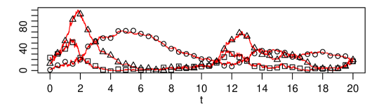
Figure 1: Observations $x^{1}_{t}$ (squares), $x^{2}_{t}$ (circles) and $x^{3}_{t}$ (triangles) of the Oregonator model for $t\in\mathbb{T}$. The true Markov jump process is indicated as solid line.

6.1.1 Specifications of the algorithm

We specify the proposal distributions and further details in our algorithm as follows. A basis vector matrix is given by

$$V(A)=\left(\begin{array}[]{ccccc}1&-1&0&1&0\\ 1&0&1&1&1\\ \end{array}\right)^{T}$$

and we simulate $Z$ in (6) with $(B_{1}\bar{B}_{1},B_{2}\bar{B}_{2})^{T}$, where $\textrm{P}[B_{l}=\pm 1]=0.5$, $\bar{B}_{l}\sim\mathrm{Bin}(2,\iota)$, $\iota=0.4$ and all random numbers are independent. For the new reaction number at the beginning on the interval $[t_{n-1},t_{n}]$ or at the end on the interval $[t_{n-1},t_{n}]$, we want updates which change only one component of $y_{t_{0}}$ or $y_{t_{n}}$, respectively, to get better acceptance. In order to do this, we need the integer solutions to

$$A_{-j,.}(r_{tot}^{new}-r_{tot})=0$$

for $j\in\{1,2,3\}$, where $A_{-j,.}$ denotes the reaction matrix without the $j$-th row. With the techniques from Appendix A, we find exemplarily for $j=1$ the basis vectors $v_{1}=(1,-1,0,0,0)^{T}$, $v_{2}=(0,0,0,1,0)^{T}$ and $v_{3}=(0,1,1,0,1)^{T}$. Because the last one is already in the kernel of $A$, we can restrict ourselves to $v_{1}$ and $v_{2}$ for the update, i.e., we choose one of these or their additive inverses with equal probability and add it to the total reaction number to get the new one. We proceed analogously for $j=2$ and $j=3$.

For the parameters $\theta$, we use $\Gamma(0.1,1)$ priors. For the scenarios B) to E), $\eta$ is unknown. We use $\eta=10$ during the initialisation and a $\Gamma(0,0)$ improper prior afterwards so that $\eta$ can be updated with Gamma distributions. For the initialisation (Algorithm 5), we use $M^{\{l\}}$ and $S^{\{l\}}$ around 100 to 200 and slight shrinking.

We use the standard set of sub-intervals described in Subsection 4.4. Without further tuning, we obtained average acceptance rates of $5\%$ - $7\%$ in all the scenarios. The running time for the 100’000 iterations of Algorithm 3.1 together with the initialisation (Algorithm 5), coded in the language for statistical computing R (see R Development Core Team, (2010)), was about 38 hours on one core of a 2.814 GHz Dual-Core AMD Opteron(tm) Processor 2220 with 32’000 MB RAM. A significant speed up is expected from coding in C.

6.1.2 Results

Figure 2: Traces for the parameters in scenario B for the Oregonator example with a thinning factor 10. The origin on the abscissa marks the last iteration of the initialisation (Algorithm 5). True values are indicated with a horizontal line.

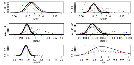
Figure 3: Posterior densities of the parameters $\theta$ and $\eta$ for the Oregonator model in the scenarios A (thick-solid), B (thin-solid), C (dashed), D (dotted) and E (dot-dashed), estimated from the last 50’000 of 100’000 iterations of Algorithm 3.1. True values are indicated with a vertical dotted line.

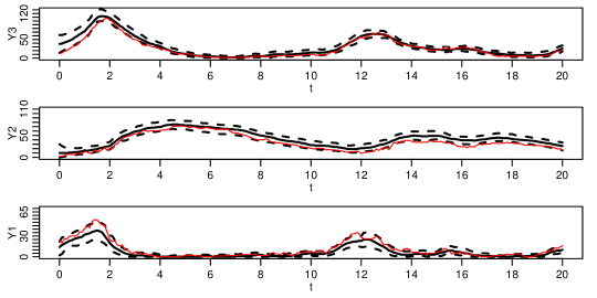
Figure 4: Estimates (thick solid lines) and point-wise 95$\%$ confidence bands (indicated by the dashed lines) of the latent components for the Oregonator model in the scenarios C (top), D (middle) and E (bottom), respectively, estimated from the last 50’000 iterations of Algorithm 3.1, thinned by a factor of 10. The true values are shown as thin line.

In Figure 2, we show the trace plots for the parameters $(\theta,\eta)$ exemplarily in scenario B. On the whole, mixing seems satisfactory, although not ideal for some parameters. In addition, we can see that the initialisation process yields starting values which are already very close to the true values.

In Figure 3, we compare the posterior densities estimated from the last 50’000 of 100’000 iterations of Algorithm 3.1 in the different scenarios. The vertical dotted line indicates the true values of $\theta$ and $\eta$, respectively. We find that in all the scenarios the true values of $\theta$ are in regions where the posterior density is high. In the cases where some component is not observable, the uncertainty is bigger, especially for the reaction rates corresponding to standardized transition intensities which depend on this component. For example in scenario E, $x^{1}$ is not observed, leading to a loss in terms of precision for reactions rates $\theta_{2}$, $\theta_{3}$ and $\theta_{4}$. The posterior densities of $\eta$ seem rather spread out, but the mode is found nicely.

Figure 4 displays estimates and point-wise 95$\%$ confidence bands of the latent components in the process for the scenarios C to E. For comparison, we also indicate the true values of the latent component with a thin line. We can see that they nicely lie within our confidence bands.

6.2 Prokaryotic auto-regulation

We look at the simplified model for prokaryotic auto-regulation introduced in Golightly and Wilkinson, (2005) and reconsidered in Golightly and Wilkinson, (2009). It is described by the following set of 8 chemical reactions.

$$\begin{array}[]{llcl}R_{1}:&\mathrm{DNA}+\mathrm{P}_{2}&\longrightarrow&\mathrm{DNA}\mathrm{P}_{2}\\ R_{2}:&\mathrm{DNA}\mathrm{P}_{2}&\longrightarrow&\mathrm{DNA}+\mathrm{P}_{2}\\ R_{3}:&\mathrm{DNA}&\longrightarrow&\mathrm{DNA}+\mathrm{RNA}\\ R_{4}:&\mathrm{RNA}&\longrightarrow&\mathrm{RNA}+\mathrm{P}\\ R_{5}:&2\mathrm{P}&\longrightarrow&\mathrm{P}_{2}\\ R_{6}:&\mathrm{P}_{2}&\longrightarrow&2\mathrm{P}\\ R_{7}:&\mathrm{RNA}&\longrightarrow&\emptyset\\ R_{8}:&\mathrm{P}&\longrightarrow&\emptyset\end{array}$$

In this system, the sum $\mathrm{DNA}\mathrm{P}_{2}+\mathrm{DNA}$ remains constant, and we assume that this constant $K$ is known and equal to 10 in our simulation. Therefore it is enough to consider the four species $y=(y^{1},y^{2},y^{3},y^{4})^{T}=(\mathrm{RNA},\mathrm{P},\mathrm{P}_{2},\mathrm{DNA})^{T}$, where $\mathrm{RNA}$, $\mathrm{P}$, $\mathrm{P}_{2}$ and $\mathrm{DNA}$ are now interpreted as numbers of the corresponding species. According to the mass action law, the standardized transition intensities are

$$h(y)=(\mathrm{DNA}\times\mathrm{P}_{2},K-\mathrm{DNA},\mathrm{DNA},\mathrm{RNA},\mathrm{P}\times(\mathrm{P}-1)/2,\mathrm{P}_{2},\mathrm{RNA},\mathrm{P})^{T}$$

and the jump matrix is given by

$$A:=\left(\begin{array}[]{cccccccc}0&0&1&0&0&0&-1&0\\ 0&0&0&1&-2&2&0&-1\\ -1&1&0&0&1&-1&0&0\\ -1&1&0&0&0&0&0&0\\ \end{array}\right).$$

As start distribution, we assume that the number of DNA molecules is uniformly distributed on $\{0,\dots,K\}$ and the other species are initially $0$. Following Golightly and Wilkinson, (2009), we again use normally distributed measurement errors, see (13). The update for $\eta$ (step 4. in Algorithm 3.1), can then be done using Gamma distributions. Also we consider three scenarios in a similar manner to the last example.

• Exact observation of every species.

• Observation of every species with errors.

• Observation of species $\mathrm{RNA}$, $\mathrm{P}$ and $\mathrm{P}_{2}$ with errors.

True values of the parameters are $\theta=(0.1,0.7,0.6,0.085,0.05,0.2,0.2,0.015)$, $\eta=0.5$ and we observe the process at the integer times $0,\dots,50$. The total raction numbers for the true underlying Markov jump process are $r_{tot}=(192,190,122,53,116,99,117,7)^{T}$.

6.2.1 Transformation of parameters

As reported in Golightly and Wilkinson, (2005) and Golightly and Wilkinson, (2009), ratios of the parameters $\theta_{1}/\theta_{2}$ and $\theta_{5}/\theta_{6}$, connected to the reversible reaction pairs $R_{1}$, $R_{2}$ and $R_{5}$, $R_{6}$, respectively, are more precise than the individual rates. We found a similar behavior also for $\theta_{3}/\theta_{7}$ and $\theta_{4}/\theta_{8}$. This is related to the fact that adding or subtracting an equal number of the corresponding reaction between two consecutive observation times does not change the values of the Markov jump chain at these time points, making it rather difficult to tell how many of these reaction events should be there from discrete observations only. This implies also that there is a strong positive dependence in the posterior between these pairs of parameters, slowing down the convergence of the algorithm.

It is therefore much better to use the following reparameterization

$$\rho_{1}=\theta_{1}+\theta_{2},\ \rho_{3}=\theta_{3}+\theta_{7},\ \rho_{5}=\theta_{4}+\theta_{8},\ \rho_{7}=\theta_{5}+\theta_{6}$$

and

$$\rho_{2}=\frac{\theta_{1}}{\theta_{1}+\theta_{2}},\ \rho_{4}=\frac{\theta_{3}}{\theta_{3}+\theta_{7}},\ \rho_{6}=\frac{\theta_{4}}{\theta_{4}+\theta_{8}},\ \rho_{8}=\frac{\theta_{5}}{\theta_{5}+\theta_{6}}.$$

We use $\Gamma(\alpha,\beta)$ priors with $\alpha=0.1$ and $\beta=1$ for $\rho_{l}$ ($l=1,3,5,7$) and $\mathrm{B}(1,1)$ priors, i.e., uniform priors on $[0,1]$, for $\rho_{k}$ ($k=2,4,6,8$). For updating e.g. $(\rho_{1},\rho_{2})$, we factor the joint density of $(\rho_{1},\rho_{2})$ given $y_{[t_{0},t_{n}]}$ as $p(\rho_{1}|\rho_{2})p(\rho_{2})$. Then $p(\rho_{1}|\rho_{2})$ is a $\Gamma(\alpha+r_{tot^{1}}+r_{tot}^{2},\beta+\rho_{2}I_{1}+(1-\rho_{2})I_{2}))$ density, and

$$p(\rho_{2})\propto(\beta+\rho_{2}I_{1}+(1-\rho_{2})I_{2})^{-(\alpha+N_{1}+N_{2})}\rho_{2}^{N_{1}}(1-\rho_{2})^{N_{2}},$$

with $I_{1}=\sum_{k=1}^{n_{tot}+1}h_{1}(y_{k-1})\delta_{k}$ and $I_{2}=\sum_{k=1}^{n_{tot}+1}h_{2}(y_{k-1})\delta_{k}$. The factor $(\beta+\rho_{2}I_{1}+(1-\rho_{2})I_{2})^{-(\alpha+N_{1}+N_{2})}$ can be approximated with piecewise linear upper bounds, so we can simulate from $p(\rho_{2})$ using an adaptive accept-reject-method with mixtures of truncated Beta distributions as proposals.

6.2.2 Specifications of the algorithm

The basis vector matrix is given by

$$V(A)=\left(\begin{array}[]{cccccccc}1&1&0&0&0&0&0&0\\ 0&0&0&0&1&1&0&0\\ 0&0&1&0&0&0&1&0\\ 0&0&0&1&0&0&0&1\\ \end{array}\right)^{T}$$

and for $q_{\iota}^{Z}$ we choose $q_{\iota}^{Z}(\pm\vec{e}_{i})=0.1$ for $i\in\{1,2,3,4\}$ and $q_{\iota}^{Z}(\vec{0})=0.2$ (see (6)).

To get the new total reaction number for the update at the beginning, i.e., on the interval $[t_{0},t_{1}]$, we have to respect that $y_{t_{0}}^{1}=y_{t_{0}}^{2}=y_{t_{0}}^{3}=0$. We therefore only want to change the fourth component of $y_{t_{0}}$. So

$$A_{-4,.}(r_{tot}^{new}(y_{[t_{0},t_{1}]})-r_{tot}(y_{[t_{0},t_{1}]}))=0.$$

With the techniques from Appendix A, we find the same basis vectors as in $V(A)$ plus the vector $v_{5}=(0,-1,0,2,1,0,0,0)^{T}$. So we use (12) with $q_{\iota}^{R}(\pm v_{5})=0.5$. Updating the total reaction number at the end on the interval $[t_{n-1},t_{n}]$ is done as in the previous example.

6.2.3 Results

Figure 5: Traces for the parameters for the prokaryotic auto-regulation model in scenario A with a thinning factor 100. The origin on the abscissa marks the last iteration of the initialisation (Algorithm 5). True values are indicated with a horizontal line.

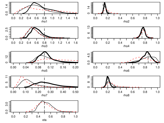
Figure 6: Posterior densities of the parameters $\rho$ and $\eta$ for the prokaryotic auto-regulation model in the scenarios A (thick-solid), B (thin-solid) and C (dashed), estimated from the last 40’000 of 50’000 iterations (thinned with factor 100) of Algorithm 3.1. True values are indicated with a vertical dotted line.

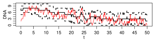
Figure 7: Estimates (thick solid lines) and 95$\%$ confidence intervals (indicated by the dashed lines) of the latent components in the scenario C (prokaryotic auto-regulation model), estimated from the last 40’000 iterations of Algorithm 3.1 thinned by a factor of 10. True values are shown as thin line.

The running time for the 50’000 iterations of Algorithm 3.1 together with the initialisation (Algorithm 5), coded in the language for statistical computing R (see R Development Core Team, (2010)), was about 16 hours on on one core of a 2.814 GHz Dual-Core AMD Opteron(tm) Processor 2220 with 32’000 MB RAM. Average acceptance rates were around $15\%$ - $25\%$.

In Figure 5, we show the trace plots of the initialisation and 50’000 iterations of Algorithm 3.1 for the scenario A. For the parameter $\rho_{1}$, the mixing is somewhat problematic.

In Figure 6, we can see, as expected, that the posterior densities of $\rho_{2}$, $\rho_{4}$, $\rho_{6}$ and $\rho_{8}$ are far more concentrated than those of $\rho_{1}$, $\rho_{3}$, $\rho_{5}$ and $\rho_{7}$. Nevertheless, all posterior densities go well with the true values. When the number of DNA molecules is not observed (scenario C), the posteriors of $\rho_{1}$ and and $\rho_{3}$ are spread out, so estimating them in this scenario seems rather hard.

Finally, we show estimate and the point-wise 95$\%$ confidence band of the latent component in scenario C, that is the number of DNA molecules, in Figure 7. The results contain the true values quite nicely.

7 Conclusions

In this paper, we have presented a technique to infer rate constants and latent process components of Markov jump processes from time series data using fully Bayesian inference and Markov chain Monte Carlo algorithms. We have used a new proposal for the Markov jump process and - exploiting the general state space framework - a filter type initialisation algorithm to render the problem computationally more tractable. Even in very data-poor scenarios in our examples, e.g. one species is completely unobserved, we have been able to estimate parameter values and processes and the true values are contained in posterior confidence bands.

The techniques are generic to a certain extend, but as our examples have shown, they have to be adapted to the situation at hand, which makes their blind application rather difficult. Clearly, the speed of our algorithm scales with the number of jump events, so they are less suitable in situations with many jumps. In such a situation, using the diffusion approximation is recommended. However, we believe that the statement “It seems unlikely that fully Bayesian inferential techniques of practical value can be developed based on the original Markov jump process formulation of stochastic kinetic models, at least given currently available computing hardware” in the introduction of Golightly and Wilkinson, (2009) is too pessimistic.

Appendix A Integer solutions of Homogeneous Linear Equations

Let $A\in M_{p\times r}(\mathbb{Z})$ be an integer $p\times r$ matrix. We want to determine the set

$$\mathbb{L}=\{x\in\mathbb{Z}^{r}:Ax=0\}.$$ (14)

Obviously, it is enough to consider only linear independent rows of $A$, so we assume $rank(A)=p\leq r$. The case $p=r$ is then trivial, so $p<r$. The main idea is to transform the matrix $A$ into the so called Hermite normal form. For the following, see Jäger, (2001).

Definition A.1 (Hermite normal form).

A matrix $H\in M_{p\times r}(\mathbb{Z})$ with rank $s$ is in Hermite normal form if

1. $\exists i_{1},\dots,i_{s}$ with $1\leq i_{1}<\dots<i_{s}\leq p$ with $H_{i_{j},j}\in\mathbb{Z}\backslash\{0\}$ for $1\leq j\leq s$.

2. $H_{i,j}=0$ for $1\leq i\leq i_{j}-1,\ 1\leq j\leq s$.

3. The columns $s+1$ to $r$ are $0$.

4. $\lfloor H_{i_{j},l}/H_{i_{j},j}\rfloor=0$ for $1\leq l<j\leq s$.

Proposition A.1.

For every $A\in M_{p\times r}(\mathbb{Z})$ exists a unique unimodular matrix $U$ ($U\in GL_{r}(\mathbb{Z}):=\{B\in M_{r\times r}(\mathbb{Z}):\det(B)=\pm 1\}$), such that $H=AU$ is in Hermite normal form.

There exist many algorithms to calculate $H$ and $U$, see e.g. Jäger, (2001).

The Hermite normal form allows us to determine the set (14). Because $A$ is assumed to have maximal rank, by definition $H=(B,0)$, where $B$ is an invertible, lower triangular $p\times p$ matrix. For $y=U^{-1}x$ we have the equation

$$0=Ax=AUy=(B,0)y,$$

so $y$ has zeroes in the first $p$ positions and arbitrary integers in the remaining positions. Hence a basis vector matrix $V$ for (14) is given by $v_{i}=u_{r+i}$. If necessary, one can reduce the length of the $v_{i}$ by the algorithm 2.3 in Ripley, (1987).

References

• Arkin et al., (1998) Arkin, A., Ross, J., and McAdams, H. H. (1998). Stochastic kinetic analysis of developmental pathway bifurcation in phage $\lambda$-infected escherichia coli cells. Genetics, 149:1633–1648.
• Bickel and Doksum, (1977) Bickel, P. J. and Doksum, K. A. (1977). Mathematical Statistics; Basic Ideas and Selected Topics. Holden-Day Inc., Oakland.
• Boys et al., (2008) Boys, R. J., Wilkinson, D. J., and Kirkwood, T. B. (2008). Bayesian inference for a discretely observed stochastic kinetic model. Statistics and Computing, 18(2):125–135.
• Doucet et al., (2001) Doucet, A., de Freitas, J. F. G., and Gordon, N. J. (2001). Sequential Monte Carlo Methods in Practice. Springer, New York.
• Durham and Gallant, (2002) Durham, G. and Gallant, R. (2002). Numerical techniques for maximum likeliood estimation of continuous time diffusion processes. Journal of Business and Economic Statistics, 20:279–316.
• Gibson and Bruck, (2000) Gibson, M. A. and Bruck, J. (2000). Efficient exact stochastic simulation of chemical systems with many species and many channels. J. Phys. Chem. A, 104(9):1876–1889.
• Gilks and Berzuini, (2001) Gilks, W. R. and Berzuini, C. (2001). Following a moving target-Monte Carlo inference for dynamic bayesian models. Journal Of The Royal Statistical Society Series B, 63(1):127–146.
• Gilks et al., (1996) Gilks, W. R., Richardson, S., and Spiegelhalter, D. J. (1996). Markov chain Monte Carlo in Practice. Chapman and Hall, London.
• Gillespie, (1977) Gillespie, D. T. (1977). Exact stochastic simulation of coupled chemial reactions. The Journal of Physical Chemistry, 81:2340–2360.
• Golightly and Wilkinson, (2008) Golightly, A. and Wilkinson, D. (2008). Bayesian inference for nonlinear multivariate diffusion models observed with error. Computational Statistics & Data Analysis, 52(3):1674 – 1693.
• Golightly and Wilkinson, (2005) Golightly, A. and Wilkinson, D. J. (2005). Bayesian inference for stochastic kinetic models using a diffusion approximation. Biometrics, 61:781–788.
• Golightly and Wilkinson, (2006) Golightly, A. and Wilkinson, D. J. (2006). Bayesian sequential inference for stochastic kinetic biochemical network models. Journal of Computational Biology, 13(3):838–51.
• Golightly and Wilkinson, (2009) Golightly, A. and Wilkinson, D. J. (2009). Markov chain Monte Carlo algorithms for sde parameter estimation. In Learning and Inference for Computational Systems Biology. MIT Press.
• Hobolt and Stone, (2009) Hobolt, A. and Stone, E. A. (2009). Simulation from endpoint-conditioned, continuous-time Markov chains on a finite state space, with applications to molecular evolution. Annals of Applied Statistics, 3(3):1204–1231.
• Jäger, (2001) Jäger, G. (2001). Algorithmen zur Berechnung der Smith-Normalform und deren Implementation auf Parallelrechnern. PhD thesis, Universität Essen.
• Künsch, (2000) Künsch, H. R. (2000). Complex Stochastic Systems, chapter 3. Chapman & Hall/CRC Press LLC.
• McAdams and Arkin, (1997) McAdams, H. and Arkin, A. (1997). Stochastic mechanisms in gene expression. Proceedings of the National Academy of Sciences of the USA, 94:814–819.
• Ogata, (1981) Ogata, Y. (1981). On Lewis’ simulation method for point processes. IEEE Transactions on Information Theory, 27(1):23–31.
• R Development Core Team, (2010) R Development Core Team (2010). R: A Language and Environment for Statistical Computing. R Foundation for Statistical Computing, Vienna, Austria.
• Ripley, (1987) Ripley, B. D. (1987). Stochastic Simulation. Wiley, NY.
• Robert and Casella, (2004) Robert, C. P. and Casella, G. (2004). Monte Carlo Statistical Methods, Second Edition. Springer Texts in Statistics. Springer Science and Business Media Inc., Spring Street, New York, NY 10013, USA, 2 edition.
• Wilkinson, (2006) Wilkinson, D. J. (2006). Stochastic Modelling for Systems Biology. Chapman & Hall.