On demand entanglement in double quantum dots via coherent carrier scattering

Abstract

We show how two qubits encoded in the orbital states of two quantum dots can be entangled or disentangled in a controlled way through their interaction with a weak electron current. The transmission/reflection spectrum of each scattered electron, acting as an entanglement mediator between the dots, shows a signature of the dot-dot entangled state. Strikingly, while few scattered carriers produce decoherence of the whole two-dots system, a larger number of electrons injected from one lead with proper energy is able to recover its quantum coherence. Our numerical simulations are based on a real-space solution of the three-particle Schrödinger equation with open boundaries. The computed transmission amplitudes are inserted in the analytical expression of the system density matrix in order to evaluate the entanglement.

1 Introduction

Among the various proposals and schemes advanced for realiable quantum computing architectures [1, 2, 3, 4], semiconductor double quantum dots (DQDs) are considered very promising candidates for the realization of quantum bits and gates [3, 4, 5, 6, 7]. Indeed, these structures can arbitrarily be scaled to large systems and could be easily integrable with other microlectronic devices. Besides their potentialities in the frame of quantum information science, DQDs are also very interesting from the basic physics point of view, as they enable both to analyze the peculiar features of electron transport phenomena, and to relate them to the appearance of quantum correlations [8, 9, 10, 11].

A number of implementations of DQDs qubits have been investigated from the theoretical and experimental points of view [3, 4, 5, 6, 7]. Two degrees of freedom, spin and charge, can be used to encode the qubit. While the feasibility of quantum logic gates acting on spin states is hampered by the need of local magnetic fields [12], state-of-the-art nanofabrication technology [13, 14, 15] allows for a precise control of the local charge and orbital degrees of freedom. Recently, Shinkay et al. [15] have realized the coherent manipulation of charge states in two spatially separated DQDs integrated in a GaAs/AlGaAs heterostructure. Specifically, multiple two-qubit operations, such as the controlled-rotation and the swap, have been successfully implemented.

The main threat to the correct functioning of quantum information processing devices is represented by the decoherence stemming from the interaction with the external environment or, from a different perspective, by the uncontrolled entanglement of the qubits with the environment. For charge states in semiconductor DQDs, the loss of coherence is mainly due to the coupling of the carriers to the crystal lattice vibrations and to the Coulomb interaction with other charged particles [16]. In fact, the decoherence induced by the electron-phonon interaction has been widely investigated in the literature [7, 17, 18, 19, 20], where the quantum dots (QDs) are usually considered as two point-like systems with two energy levels coupled to the phonon bath. Analytical estimations of the decoherence effects and of their characteristic timescales have been given by using various techniques, ranging from the Born-Markov approximation [17] to perturbative calculations in a non-Markovian regime [7, 18]. On the other hand, the role played by the Coulomb interaction between charge carriers into the loss of coherence has not been deeply analyzed.

In this paper, we intend to investigate the entanglement properties of bound electrons in a GaAs DQD when other electron pass through the structure. In particular, we focus on the appearance of quantum correlations in a three-particle scattering, where charged particles incoming from a lead enter, one at a time, in a DQD structure and interact via Coulomb potential with two electrons, one in each dot. In our scheme, the electrons crossing the device have the double role of entanglement “mediator” between the two dots and between the DQDs system and the leads, i.e. the environment. The aim of this work is to show how the Coulomb interaction between the system and the “mediator” can be, under certain conditions, a suitable means to entangle or disentangle in a controlled way the qubit states encoded in the single-particle energy levels of the dots. A detailed theoretical estimation of such effects results to be of interest also for the experimental feasibility of the above qubit, as the results reached in the production, manipulation, and coherent control of charge states in DQDs seem to indicate [13, 14, 15]. In this view the entanglement/disentanglement of the DQDs can be connected to the precise engineering or the suitable tuning of physical and geometrical parameters, such as the DQDs level spacing or the current intensity, here modelled as the successive injection of carriers in the scattering region.

The numerical procedure used to solve the model is a generalization of the quantum transmitting boundary method (QTBM) [21, 22]. It allows us to find the reflection and transmission amplitudes of each scattering channel as a function of the initial kinetic energy of the incoming carrier and of the state occupation of the dots. Our analysis is time-independent, in the sense that the few-particle scattering states are obtained by the solution of a time-independent open-boundary Schrödinger equation, and therefore does not permit to evaluate the dynamics and the characteristic timescales of quantum correlations [22, 23]. On the other hand, the QTBM takes explicitely into account the spatial structure and therefore the size and the shape of the dots, thus permitting to overcome the approximations implied in the description of a dot in terms of a two-level point-like system. We single-out the peculiar mechanisms of electron transport through DQDs resulting in resonances in the transmission and reflection spectra and thus leading to entanglement and decoherence [24, 25, 23, 26, 27]. In the evaluation of such effects, both the transmitted and reflected components of the scattered wavefunction are taken into account.

The paper is organized as follows. In Section 2, we introduce the physical system reproducing a DQD structure in GaAs, and illustrate the computational approach adopted to find the few-particle scattering states. The description of the DQD in terms of a two-qubit model and the discussion about the theoretical procedures used to evaluate the entanglement and the decoherence are given in Section 3. In Section 4, we show the numerical results first obtained for the scattering of a single carrier, then for a weak electric current. For the latter case, the condition leading to the maximum entanglement production or to the complete disentanglement are analyzed in detail. Finally, in Section 5 we comment on the results and draw our conclusions.

2 The DQD structure and the computational approach

In our model (see Figure 1), we consider an electron incoming from the left, with respect to the DQD one dimensional (1D) structure, with kinetic energy $T_{0}$. We examine the case of one scattered carrier at a time, i.e. we suppose that an electron enters the scattering region only after the previous one has already left. Such an assumption, and the fact that the charging energy of the DQD is larger than the spacing between the two-particle energy levels, means that our system always operates in three-particle regime. The incident particle is scattered via Coulomb interaction by the two electrons bound in a structure potential $V_{s}$ in a region of length $L$ (Figure 1) mimicking a DQD structure and constituted by two potential wells separated by a potential barrier wide enough to make negligible the Coulomb interaction between the two confined particles. Moreover, the structure is connected to external leads kept at zero potential. The $N$ two-particle bound states and energies of the DQD will be indicated by $|\Xi_{n}\rangle$ and $\epsilon_{n}$, respectively (with $n$0 indicating the ground state). As it will be shown in the following, some of them can also be expressed in terms of $|\chi_{l}^{R}\chi_{m}^{L}\rangle$ and $(E_{l}^{R}+E_{m}^{L})$, where $|\chi_{l}^{R}\rangle(|\chi_{m}^{L}\rangle)$ indicates the single-particle bound state of the right (left) dot with energy $E_{l}^{R}(E_{m}^{L})$. Due to the symmetry of the potential $V_{s}$, $E_{l}^{R}=E_{l}^{L}$.

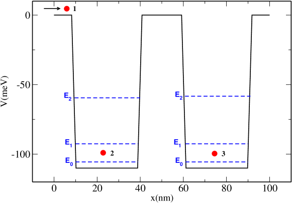
Figure 1: Profile of the potential $V_{s}(x)$ in the scattering region of length $L$=100 nm: the two potential wells are 110 meV deep and 30 nm wide and are separated by a 20 nm barrier. The dashed lines indicate the single-particle energy levels $E_{0}$, $E_{1}$, and $E_{2}$ of the ground, the first and second excited state of the dots respectively, with $E_{0}$=-105.6 meV,$E_{1}$=-92.5, and $E_{2}$=-71.5 meV. With our parameters the levels $E_{2}$ (and above) are found to have negligible occupancy. In our numerical calculations we take $m^{\ast}$=0.067 $m_{e}$, with $m_{e}$ indicating the bare mass electron, and $\varepsilon$=12.9.

As anticipated, we restrict our investigation to a 1D analysis. Such an assumption, needed to solve numerically the few-particle problem with open boundaries, is physically reasonable if the transverse dimension of the structure is small compared with the other length scales. In this case, all the particles can be supposed to occupy the lowest single-particle transverse subband [28]. Furthermore, we consider for the incoming electrons only energies below the ionization threshold of the DQD. This means that when the outgoing electrons leave the scattering region, either reflected or transmitted, the confined particles remain in a bound state of the DQD.

The three-particle Hamiltonian $\mathcal{H}$ is given by

$$\mathcal{H}(x_{1},x_{2},x_{3})=\mathcal{H}_{0}(x_{1})+\mathcal{H}_{0}(x_{2})+\mathcal{H}_{0}(x_{3})+\sum_{i=1}^{3}\sum_{j=1}^{i-1}\frac{e^{2}}{4\pi\varepsilon r_{ij}}\exp{(-r_{ij}/\lambda_{d})},$$ (1)

where $r_{ij}=\sqrt{\left(x_{i}-x_{j}\right)^{2}+d^{2}}$ and $\mathcal{H}_{0}(x_{i})$ is the single-particle Hamiltonian

$$\mathcal{H}_{0}(x_{i})=-\frac{\hbar^{2}}{2m^{\ast}}\frac{\partial^{2}}{\partial x_{i}^{2}}+V_{s}(x_{i}).$$ (2)

$\varepsilon$ and $m^{\ast}$ are the dielectric constant and effective mass of the GaAs, respectively. The term describing the mutual interaction between particles in the r.h.s. of equation (1) is a screened Coulomb potential with a Debye length $\lambda_{d}$, here taken significantly larger than the characteristics length of the structure. Furthermore, the Coulomb term also accounts for the transversal dimension $d$ of the confined system (with $d$=1 nm) through a cut-off term. In our approach, the fermionic nature of the carriers is explicitly accounted for by antisymmetrizing the two- and three-particle wavefunctions $\Xi_{n}(x_{2},x_{3})$ and $\Psi(x_{1},x_{2},x_{3})$ for any two-particle exchange. It is worth noting that the Hamiltonian given in equation (1) does not include spin-orbit terms. As a consequence, since the orbital wavefunction is antisymmetric, we are simulating a three-particle system with a symmetric spin component, as in the case of three spin-up (or spin-down) electrons. Furthermore, we do not include electron-phonon interaction. Infact, the aim of our work is to investigate the role played by the Coulomb interaction among the electrons in the system into the appearance of entanglement and decoherence. Our device is supposed to operate at a temperature in mK regime, where only spontaneous emission is effective and ignoring the coupling of the electrons with the surrounding crystal lattice does not constitute a crucial approximation, as we will describe in the following. In GaAs-based structures with levels splitting of few meV, single-phonon processes lead to an excited-state lifetime of the order of 10^-10 s, while multi-phonon and multi-electron processes are orders of magnitude less frequent (see References [29, 30]). Given a kinetic energy of 15 meV, a single electron traverse our 100 nm long device in about 10^-13 s. If we suppose independent electrons injected from the lead at a mean rate of one every 10^-12 s, corresponding to a current of about 0.16 $\mu$A, 100 carriers can be scattered through the double-dot before a phonon-induced relaxation takes place. As a consequence, in the following sections where we consider a weak electric current, we will limit our calculation up to 60 electrons.

The scattering states of the three particles are obtained by solving the time-independent open-boundary Schrödinger equation $\mathcal{H}\Psi=E\Psi$ in the cubic domain $\big{\{}x_{1},x_{2},x_{3}\big{\}}$ with $x_{i}\in[0,L]$ and with the Hamiltonian $\mathcal{H}$ given in equation (1). For this purpose, we applied a few-particle generalization of the so-called QTBM [21], allowing one to include proper open-boundary conditions for each edge of the domain. These describe the particle coming from the left as a plane wave with energy $T_{0}$ and wavevector $k_{0}$ while the other two electrons are set in a two-particle bound state $|\Xi_{j}\rangle$ of the DQD with energy $\epsilon_{j}$. Moreover, to account for the exchange symmetry of the three-particle wavefunction, also the antisymmetry of the boundary conditions is imposed, as shown in previous works [22, 23].

The correlated scattering state when the particle $1$ is localized in the left lead (that is $x_{1}<0$) reads

$$\Psi(x_{1},x_{2},x_{3})\bigg{|}_{(x_{1}<0)}=$$

$$\Xi_{j}(x_{2},x_{3})e^{ik_{0}x_{1}}+\sum_{n=0}^{M}b_{jn}\Xi_{n}(x_{2},x_{3})e^{-ik_{(j-n)}x_{1}}+\sum_{n=M+1}^{\infty}b_{jn}\Xi_{n}(x_{2},x_{3})e^{k_{(j-n)}x_{1}}$$ (3)

where $j=0\ldots N$ is the index of the initial two-particle DQD state. Analogously, when the particles 2 and 3 are in the left lead, the boundary conditions are $\Psi(x_{1},x_{2},x_{3})|_{(x_{2}<0)}$=$-\Psi(x_{2},x_{1},x_{3})|_{(x_{2}<0)}$ and $\Psi(x_{1},x_{2},x_{3})|_{(x_{3}<0)}$= $\Psi(x_{3},x_{1},x_{2})|_{(x_{3}<0)}$, respectively. In the above expression $k_{(j-n)}$=$\sqrt{2m^{\ast}T_{(j-n)}}$, where $T_{(j-n)}$ denotes the kinetic energy of an electron freely propagating in the lead, as obtained by energy conservation $T_{(j-n)}=T_{0}+\epsilon_{j}-\epsilon_{n}$. For sake of simplicity, we set $\hbar$=1 here and in the following.

The first term appearing in the r.h.s of equation (2) describes electron 1 incoming from the left lead as a plane wave with energy $T_{0}$, while the other electrons are in the two-particle bound state $|\Xi_{j}\rangle$. The second term represents the linear combination of all the energetically-allowed possibilities when particle 1 is reflected back as a plane wave with wave vector $k_{(j-n)}$ and the DQD is in the state $|\Xi_{n}\rangle$. $M$ indicates the number of states for which $T_{(j-n)}\geq 0$. The last term accounts for those states with $T_{(j-n)}$ negative, which describe particle 1 as an evanescent wave in the left lead. Therefore, the coefficients $b_{jn}$ are the transition amplitudes between the initial state $\Xi_{j}(x_{2},x_{3})e^{ik_{0}x_{1}}$ and the final state $\Xi_{n}(x_{2},x_{3})e^{ik_{(j-n)}x_{1}}$ when the incoming carrier is reflected.

If particle 1 is in the right lead, the three-particle wavefunction takes a form similar to expression (2), which describes the outgoing travelling and evanescent modes of the electron in the right lead ($x_{1}>L$):

$$\Psi(x_{1},x_{2},x_{3})\bigg{|}_{(x_{1}>L)}=\sum_{n=0}^{M}c_{jn}\Xi_{n}(x_{2},x_{3})e^{ik_{(j-n)}x_{1}}+\sum_{n=M+1}^{\infty}c_{jn}\Xi_{n}(x_{2},x_{3})e^{-k_{(j-n)}x_{1}},$$ (4)

while $\Psi(x_{1},x_{2},x_{3})|_{(x_{2}>L)}$=$-\Psi(x_{2},x_{1},x_{3})|_{(x_{2}>L)}$ for $x_{2}>L$ and $\Psi(x_{1},x_{2},x_{3})|_{(x_{3}>L)}$=
$\Psi(x_{3},x_{1},x_{2})|_{(x_{3}>L)}$ for $x_{3}>L.$ The coefficients $c_{jn}$ describe the transition amplitudes in the $n$-th channel, i.e. when the bound particles are in the $n$-th state of the DQD. The boundary conditions are given by equations (2) and (4) with $x_{1}$=0 and $x_{1}$=$L$. They are coupled to the Schrödinger equation and discretized by a finite-difference method. A system of seven equations is obtained, whose numerical solution provides the unknown coefficients $b_{jn}$ and $c_{jn}$, and the three-particle wavefunction $\Psi(x_{1},x_{2},x_{3})$ in the internal points.

3 Decoherence and entanglement of the two-qubit model

As a consequence of the scattering, quantum correlations between the single-particle energy levels of the bound electrons and the energies of the scattered electron appear. They are responsible both for the loss of quantum coherence of the two-particle state of the DQD and for the building up of quantum entanglement between the two dots. First, we show that under some approximations the DQD system can be reduced to a two-qubit model. Then, we describe in detail the theoretical approach used to evaluate entanglement and decoherence in such a model.

Although the fermionic nature of the carriers has been explicitly taken into account, as shown in Section 2, in order to solve numerically the physical system, we do not use entanglement criteria for identical particles [31, 32, 33]. In fact, the scattered carrier, either transmitted or reflected, can be assumed to be far from the scattering region, while the bound particles are essentially trapped into two deep potential wells far away from each other. So the spatial overlap between the particles results to be negligible. Therefore, the position variables can be used to distinguish the particles, while quantum correlations are evaluated between scattering channels [34, 23]. By moving from spatial to energy representation for the quantum states, and taking as input state $|\Phi_{IN}\rangle$=$|T_{0}\epsilon_{j}\rangle$, which describes the carrier incoming from the left lead with kinetic energy $T_{0}$ and the particles bound with energy $\epsilon_{j}$, the output $|\Phi_{OUT}\rangle$ reads

$$|\Phi_{OUT}\rangle=\sum_{n=0}^{M}\tilde{b}_{jn}|T_{(j-n)}^{<}\epsilon_{n}\rangle+\sum_{n=0}^{M}\tilde{c}_{jn}|T_{(j-n)}^{>}\epsilon_{n}\rangle$$ (5)

where the coefficients $\tilde{b}_{jn}$ are given by $\tilde{b}_{jn}=b_{jn}/(\sum_{n=0}^{M}(|b_{jn}|^{2}+|c_{jn}|^{2})$, and the analogous expression holds for $\tilde{c}_{jn}$, while $|T_{(j-n)}^{<(>)}\epsilon_{n}\rangle$ indicates the state with the carrier reflected (transmitted) as a plane wave (with kinetic energy $T_{(n-j)}=k_{(n-j)}^{2}/2m$) and the other two electrons bound in $|\Xi_{n}\rangle$ with energy $\epsilon_{n}$. It is worth noting that in the above expression we have omitted the reflected and transmitted outgoing evanescent modes, since their contribution to the total current is zero and cannot be responsible of any entanglement.

So far, we considered the case of the injection of a single carrier in the scattering region when the two particles trapped in the DQD structure are described by a pure state. Let us now examine the injection of a second electron also with kinetic energy $T_{0}$ in the scattering region, occurring after the exit of the previous one from the DQD structure via transmission or reflection. We indicate as $a$ and $b$ the first and the second injected electron, respectively. When $b$ enters the DQD, the bound electrons are not in a two-particle pure state, since they are coupled to the energy levels of the carrier $a$, as shown by equation (5). Therefore, the scattering between the electron $b$ and the other two bound in the DQD, will give the four-particle state

$$|\Phi_{OUT}^{(b,a)}\rangle=\sum_{n=0}^{M}\sum_{m=0}^{M}\tilde{b}_{jn}\tilde{b}_{nm}|{T_{(n-m)}^{\prime<}}{T_{(j-n)}^{<}}\epsilon_{m}\rangle+\sum_{n=0}^{M}\sum_{m=0}^{M}\tilde{b}_{jn}\tilde{c}_{nm}|{T_{(n-m)}^{\prime>}}{T_{(j-n)}^{<}}\epsilon_{m}\rangle$$

$$+\sum_{n=0}^{M}\sum_{m=0}^{M}\tilde{c}_{jn}\tilde{b}_{nm}|{T_{(n-m)}^{\prime<}}{T_{(j-n)}^{>}}\epsilon_{m}\rangle+\sum_{n=0}^{M}\sum_{m=0}^{M}\tilde{c}_{jn}\tilde{c}_{nm}|{T_{(n-m)}^{>}}^{(b)}{T_{(j-n)}^{\prime>}}\epsilon_{m}\rangle,$$ (6)

where $T_{(n-m)}^{\prime}$=$T_{0}^{\prime}+\epsilon_{n}-\epsilon_{m}$ and $T_{l}^{\prime}$ has the same meaning of $T_{l}$ but refers to the second scattered particle, i.e. electron $b$. As more electrons are scattered, the output state describing the system involves more and more terms corresponding to the various scattering channels. For the sake of simplicity, here we only describe the theoretical procedure used to calculate entanglement and decoherence in the case of the injection of a single carrier. In the subsection 4.2, the evaluation of decoherence and entanglement due to the interaction with a large number of injected carriers (mimicking an electric current) will be given for a specific case.

In order to compute the non-separability degree of the DQD system into the product of single-particle states of the dots, that is the dot-dot entanglement, we have to move from the description of the the DQD in terms of two-particle bound states to the description in terms of single-particle bound states of the left and right dots. Thanks to the negligible Coulomb interaction between the two dots of Figure 1, the four lowest two-particle orbital states $|\epsilon_{n}\rangle$ can be written in terms of single-particle states $|E_{l}^{R}\rangle$ and $|E_{m}^{L}\rangle$, of the right and left dot, respectively (Table 1).

Table 1: The table displays the scalar product $\langle E_{n}^{L}E_{m}^{R}|\epsilon_{l}\rangle$ for some values of $n,m,l$.

• 	$|E_{0}^{L}E_{0}^{R}\rangle$	$|E_{0}^{L}E_{1}^{R}\rangle$	$|E_{1}^{L}E_{0}^{R}\rangle$	$|E_{1}^{L}E_{1}^{R}\rangle$
  $|\epsilon_{0}\rangle$	1	0	0	0
  $|\epsilon_{1}\rangle$	0	$-\frac{1}{\sqrt{2}}$	$-\frac{1}{\sqrt{2}}$	0
  $|\epsilon_{2}\rangle$	0	$-\frac{1}{\sqrt{2}}$	$\frac{1}{\sqrt{2}}$	0
  $|\epsilon_{3}\rangle$	0	0	0	1

In particular, $|\epsilon_{0}\rangle$ is the product of the ground states of the two dots, while $|\epsilon_{1}\rangle$ and $|\epsilon_{2}\rangle$ are degenerate, being each a linear superposition of $|E_{0}^{L}E_{1}^{R}\rangle$ and $|E_{1}^{L}E_{0}^{R}\rangle$, which represent one electron in the ground state of one dot and the other in the first excited state of the other. $|\epsilon_{3}\rangle$ corresponds to the first excited states of the two dots. States with two electrons in the same dot are included in our calculations but have always a negligible occupancy. This means that the coefficients $\tilde{b}_{jn}$, and $\tilde{c}_{jn}$ with $j>3$ or $n>3$ on the right hand side of the equation (5) are 0. For our numerical calculations, we used the physical parameters of the GaAs material and the DQD potential reported in the caption of Figure 1.

In fact, we restrict our analysis to energies of the incoming particle which enable up to four scattering channels, i.e. the maximum value of $M$ in the expression (5) is 3. Under these assumptions a system of two qubits is obtained, in the sense that each confined particle can be described in terms of two states: the ground $E_{0}^{L(R)}$ and first excited $E_{1}^{L(R)}$ energy level of the left (right) QD, encoding the $|0_{L(R)}\rangle$ and $|1_{L(R)}\rangle$ states, respectively. Thus, the three-particle quantum state of equation (5) can be written as:

$$|\Phi_{OUT}\rangle=\tilde{b}_{j0}|T_{j}^{<}0_{L}0_{R}\rangle-\frac{\tilde{b}_{j1}+\tilde{b}_{j2}}{\sqrt{2}}|T_{j-1}^{<}0_{L}1_{R}\rangle-\frac{\tilde{b}_{j1}-\tilde{b}_{j2}}{\sqrt{2}}|T_{j-1}^{<}1_{L}0_{R}\rangle+\tilde{b}_{j3}|T_{j-3}^{<}1_{L}1_{R}\rangle$$

$$+\tilde{c}_{j0}|T_{j}^{>}0_{L}0_{R}\rangle-\frac{\tilde{c}_{j1}+\tilde{c}_{j2}}{\sqrt{2}}|T_{j-1}^{>}0_{L}1_{R}\rangle-\frac{\tilde{c}_{j1}-\tilde{c}_{j2}}{\sqrt{2}}|T_{j-1}^{>}1_{L}0_{R}\rangle+\tilde{c}_{j3}|T_{j-3}^{>}1_{L}1_{R}\rangle$$ (7)

where $|T_{j-1}^{>}\rangle$=$|T_{j-2}^{>}\rangle$ and $|T_{j-1}^{<}\rangle$=$|T_{j-2}^{<}\rangle$, deriving from $E_{0}^{L}+E_{1}^{R}$=$E_{1}^{L}+E_{0}^{R}$ and energy conservation has been taken into account.

The decoherence undergone by the electrons confined in the dots can be interpreted in terms of the lack of knowledge of their quantum state due to the interaction with the environment, namely the injected carrier [35]. In other words, due to the coupling between the energy states stemming from the scattering event, the two-particle DQD cannot be described by a pure state anymore but becomes a statistical mixture. A good measure of the degree of uncertainty about such a system and therefore of its loss of coherence, is given by the von Neumann entropy of the two particle reduced density matrix $\rho_{r}$, obtained by tracing the three-particle density matrix $\rho=|\Psi_{OUT}\rangle\langle\Psi_{OUT}|$ over the degrees of freedom $T_{l}^{>(<)}$ of the scattered carrier [35]. After the first scattering, the matrix representation of $\rho_{r}$ in the standard basis $\mathcal{B}=\{|0_{L}0_{R}\rangle,|0_{L}1_{R}\rangle,|1_{L}0_{R}\rangle,|1_{L}1_{R}\rangle\}$ reads

$$\rho_{r}=\left(\begin{array}[]{cccc}|\alpha|^{2}&0&0&0\\ 0&|\beta_{+}|^{2}+|\gamma_{+}|^{2}&\beta_{+}\beta_{-}^{\ast}+\gamma_{+}\gamma_{-}^{\ast}&0\\ 0&\beta_{+}^{\ast}\beta_{-}+\gamma_{+}^{\ast}\gamma_{-}&|\beta_{-}|^{2}+|\gamma_{-}|^{2}&0\\ 0&0&0&|\omega|^{2}\end{array}\right),$$ (8)

where

$$|\alpha|^{2} = |\tilde{b}_{j0}|^{2}+|\tilde{c}_{j0}|^{2}$$

$$\beta_{\pm} = \frac{\tilde{b}_{j1}\pm\tilde{b}_{j2}}{\sqrt{2}}$$

$$\gamma_{\pm} = \frac{\tilde{c}_{j1}\pm\tilde{c}_{j2}}{\sqrt{2}}$$

$$|\omega|^{2} = |\tilde{b}_{j3}|^{2}+|\tilde{c}_{j3}|^{2}.$$ (9)

In order to obtain the expression (8), the orthogonality relations between the states of the scattered carrier, $\langle T_{i}^{>(<)}|T_{j}^{>(<)}\rangle=\delta_{ij}$ and $\langle T_{i}^{<}|T_{j}^{>}\rangle=0\quad\forall\,ij$, have been used.

The decoherence $\xi$ can be evaluated by means of the von Neumann entropy as:

$$\xi=-\textrm{Tr}\left[\rho_{r}\ln{\rho_{r}}\right]=-|\alpha|^{2}\ln{|\alpha|^{2}}-\eta_{+}\ln{\eta_{+}}-\eta_{-}\ln{\eta_{-}}-|\omega|^{2}\ln{|\omega|^{2}},$$ (10)

where

$$\eta_{\pm}=\frac{1}{2}\bigg{(}|\beta_{+}|^{2}+|\gamma_{+}|^{2}+|\beta_{-}|^{2}+|\gamma_{-}|^{2}$$

$$\pm\sqrt{(|\beta_{+}|^{2}+|\gamma_{+}|^{2}+|\beta_{-}|^{2}+|\gamma_{-}|^{2})^{2}-|\beta_{+}\gamma_{-}-\beta_{-}\gamma_{+}|^{2}}\bigg{)}.$$ (11)

It ranges from 0 to $\ln{3/2}$. For $\xi$=$0$ the two bound particles can be found in a single energy level and this implies that no correlation is build up between them and the scattered carrier. When the decoherence reaches its maximum, the DQD is found in a statistical mixture of the three allowed energies $\epsilon_{0}$, $\epsilon_{1}$, and $\epsilon_{3}$ with equal weight ($\epsilon_{2}$ is equal to $\epsilon_{1}$). This implies that the uncertainty about the system is maximum.

The reduced density matrix $\rho_{r}$ describing the bound particles is also used to evaluate the dot-dot entanglement through Wootters concurrence $C$. [36] The latter is adopted to quantify the quantum correlations appearing between two qubits which cannot be described by a pure two-qubit state because of their coupling with an external environment, like in our scenario. $C$ is obtained from the density matrix $\rho_{r}$ of the two-qubit system as [36, 37]:

$$C=\max{\left\{0,\sqrt{\lambda_{1}}-\sqrt{\lambda_{2}}-\sqrt{\lambda_{3}}-\sqrt{\lambda_{4}}\right\}},$$ (12)

where $\lambda_{i}$ are the eigenvalues of the matrix $\zeta=\rho_{r}\left(\sigma_{y}^{L}\otimes\sigma_{y}^{R}\right)\rho_{r}^{\ast}\left(\sigma_{y}^{L}\otimes\sigma_{y}^{R}\right)$ arranged in decreasing order. Here $\sigma_{y}^{L(R)}$ is the Pauli matrix $\bigg{(}\begin{array}[]{cc}0&-i\\ i&0\\ \end{array}\bigg{)}$ in the basis $\{|0_{L(R)}\rangle,|1_{L(R)}\rangle\}$, and $\rho_{r}^{\ast}$ describes the complex conjugation of $\rho_{r}$ in the standard basis $\mathcal{B}$. The concurrence varies from $C$=0 for a disentangled state to $C$=1 for a maximally entangled state.

The reduced density matrix $\rho_{r}$ given in equation (8) shows an $\mathrm{X}$ structure, that is it contains non-zero elements only along the main diagonal and anti-diagonal. As shown in Ref. [38], for such a class of density matrices the concurrence can be easily evaluated and in the case of $\rho_{r}$ it becomes:

$$C=2\max{\left\{0,k\right\}},$$ (13)

where

$$k=\left|\beta_{+}\beta_{-}^{\ast}+\gamma_{+}\gamma_{-}^{\ast}\right|-|\alpha||\omega|=$$

$$\frac{1}{2}\left|(\tilde{b}_{j1}+\tilde{b}_{j2})(\tilde{b}^{\ast}_{j1}-\tilde{b}^{\ast}_{j2})+(\tilde{c}_{j1}+\tilde{c}_{j2})(\tilde{c}^{\ast}_{j1}-\tilde{c}^{\ast}_{j2})\right|-\sqrt{\left(|\tilde{b}_{j0}|^{2}+|\tilde{c}_{j0}^{2}|\right)\left(|\tilde{b}_{j3}|^{2}+|\tilde{c}_{j3}^{2}|\right)}.$$ (14)

$C$ is equal to 0 for $|\alpha||\omega|\geq|\beta_{+}\beta_{-}^{\ast}+\gamma_{+}\gamma_{-}^{\ast}|$, while it reaches its maximum value 1 if and only if $|\beta_{+}\beta_{-}^{\ast}+\gamma_{+}\gamma_{-}^{\ast}|$=1 and $|\alpha|$=$|\omega|$=0 (and therefore the coefficients $\tilde{b}_{j0}$, $\tilde{c}_{j0}$, $\tilde{b}_{j3}$ and $\tilde{c}_{j3}$ vanish). In the latter case, the two-qubit system reduces to a Bell-like state $1/\sqrt{2}\bigg{(}|0_{L}1_{R}\rangle+e^{i\theta}|1_{L}0_{R}\rangle\bigg{)}$.

4 Results and discussion

Here we analyze our numerical results on the decoherence $\xi$ undergone by the DQD system and the dot-dot entanglement $C$. We stress again that the former corresponds to the entanglement of the DQD electrons with the transmitted/reflected one, while the latter is the concurrence between the two bound electrons. In order to single-out the specific mechanisms leading to the appearance of quantum correlations, the transmission and reflection spectra have been examined.

4.1 Scattering by a single carrier

The system has been solved for the potential profile $V_{s}(x)$ sketched in Figure 1 for various input states with different energy of the incoming carrier $T_{0}$. In the top-left and bottom-left panels of Figure 2 we report the modulus of the transmission (TCs) and reflection coefficients (RCs) of the various scattering channels (that correspond the energy levels of the two-particle DQDs system) for the input states $|T_{0}\epsilon_{0}\rangle$ and $|T_{0}\epsilon_{2}\rangle$, respectively, when the incoming electron is injected with a kinetic energy ranging from 13 to 19 meV.

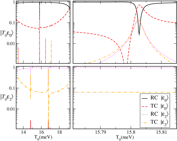
Figure 2: Left panels: Modulus of the TC and RC of the channels corresponding to the DQD levels $|\epsilon_{0}\rangle$ and $|\epsilon_{2}\rangle$ as a function of the initial kinetic energy of the incident electron $T_{0}$, ranging from 13.2 to 19.2 meV, for two different input states, namely $|T_{0}\epsilon_{0}\rangle$ (top), and $|T_{0}\epsilon_{2}\rangle$ (bottom): RC of the channel $|\epsilon_{0}\rangle$ (solid line), TC of the channel $|\epsilon_{0}\rangle$ (dashed line), RC of the channel $|\epsilon_{2}\rangle$ (dotted line), TC of the channel $|\epsilon_{2}\rangle$(dot-dashed line). The modulus of TC and RC corresponding to the other two dot states $|\epsilon_{1}\rangle$ and $|\epsilon_{3}\rangle$, are zero in the region around the resonance energy $T_{0}$= 15.8 meV: for the sake of clarity, they have not been reported. Note that the sum of the moduli of the TC and RC is 1. Right panels: Modulus of the TC and RC of the channels $|\epsilon_{0}\rangle$ and $|\epsilon_{2}\rangle$ against $T_{0}$ close to the resonant energy $\bar{T}_{0}$ for the input states $|T_{0}\epsilon_{0}\rangle$ (top), and $|T_{0}\epsilon_{2}\rangle$ (bottom).

We recall that the two-dot excited state $|\epsilon_{2}\rangle$ can be written in terms of the qubit states as $|\epsilon_{2}\rangle=1/\sqrt{2}\bigg{(}|0_{L}1_{R}\rangle-|1_{L}0_{R}\rangle\bigg{)}$, i.e. it is a Bell state. The TCs and RCs are related to the coefficients $\tilde{b}_{jn}$ and $\tilde{c}_{jn}$ given in the expression (5). For both the input configurations, sharp peaks are present only in small energy interval of the reflection and transmission spectra. It is worth noting that for different input states, such peaks appear at different values of $T_{0}$.

To get a better insight into resonances, a zoom of the modulus of TC and RC for the various channels in the energy interval around the resonant condition $\bar{T}_{0}$=15.8 meV is displayed in the right panels of the Figure 2. While for the input state $|T_{0}\epsilon_{2}\rangle$ no resonance is present in this range and the sum of the moduli of TC and RC of the channel is equal to 1, for $|T_{0}\epsilon_{0}\rangle$ the spectra show a number of sharp resonances (see the top-right panel of Figure 2). In particular the probabilities of finding the DQD in the state $|\epsilon_{2}\rangle$ (with the scattered carrier, either reflected or transmitted) shows a symmetric Lorentzian peak around $\bar{T}_{0}$, while the TCs and RCs of the scattering channel $|\epsilon_{0}\rangle$ exhibit a minimum. Specifically, the RC presents a symmetric line-shape, and the TC an asymmetric one. This behavior clearly indicates that in the transmission and reflection spectra different kind of resonances appear, namely Breit-Wigner [39] and Fano [40], respectively which have a strong connection into into the building up of quantum correlations, as noted elsewhere [23, 41, 42]. The first ones, exhibiting symmetric Lorentzian peaks, stem from the coupling of a quasi bound state to the scattering states of the leads, while the second ones, characterized by asymmetric lineshapes, are present when two competing scattering mechanisms, a resonant one and a nonresonant one, interfere, and are due to electron-electron correlation [22, 23].

Scattering resonances are a signature of peculiar decohering and entangling effects [23], as shown in Figure 3, where the dependence of DQD decoherence $\xi$ and dot-dot entanglement $C$ are reported as a function of the initial energy of the incoming electron around $\bar{T}_{0}$ for the input states $|T_{0}\epsilon_{0}\rangle$ and $|T_{0}\epsilon_{2}\rangle$.

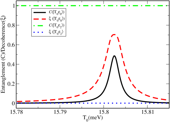
Figure 3: Dot-dot entanglement $C$ and DQD decoherence $\xi$ against the initial kinetic energy $T_{0}$ of the incident electron around the resonance condition $\bar{T}_{0}$, for two different input states: $C(|T_{0}\epsilon_{0}\rangle)$ (solid line), $\xi(|T_{0}\epsilon_{0}\rangle)$ (dashed line), $C(|T_{0}\epsilon_{2}\rangle)$ (dash-dotted line), and $\xi(|T_{0}\epsilon_{2}\rangle)$ (dotted line).

For $|T_{0}\epsilon_{2}\rangle$, the decoherence is practically zero while the entanglement remains 1, as in the initial state. In fact, as can be gathered by the behavior of TC and RC, the only coefficients not vanishing in equation (5) are $\tilde{b}_{22}$ and $\tilde{c}_{22}$, and the output state $|\Psi_{OUT}\rangle$ of expression (3) reduces to

$$|\Psi_{OUT}\rangle=-\left(\tilde{b}_{22}|T^{<}_{0}\rangle+\tilde{c}_{22}|T^{>}_{0}\rangle\right)\frac{1}{\sqrt{2}}\left(|0_{L}1_{R}\rangle+|1_{L}0_{R}\rangle\right).$$ (15)

This is the factorizable product of a single-particle state of the scattered carrier and a two-qubit state describing the bound particles in the DQD, being the latter a Bell state. This means that the entanglement between electrons confined in the dots maintains its maximum value and also that the quantum information about the DQD system is maximal since it is in a pure two-particle state. Thus, the scattering event “preserves” the entanglement between the dots while the decoherence effects result to be negligible. Such a behavior, evidencing the existence of decoherence-free entangled states of two qubits, has been widely discussed in a number of works, which stressed the key role played by the symmetric coupling of the qubits with the environment into preserving their coherence [43, 44, 45, 46]

When the input state is $|T_{0}\epsilon_{0}\rangle$, both decoherence $\xi$ and entanglement $C$ show a maximum where RC and TC of the channel $|\epsilon_{2}\rangle$ are resonant (see the top-right panel of Figure 2). In particular $\xi$ reaches $\ln{2}$. Such a value is obtained when the DQD states are maximally coupled only to the energy levels $T_{0}$ and $T_{-2}$ of the scattered carrier and this occurs when the probabilities that the scattering leaves the bound particles in their ground $|\epsilon_{0}\rangle$ or excited $|\epsilon_{2}\rangle$ state are equal. Thus the output state can be written as

$$|\Psi_{OUT}\rangle=\left(\tilde{b}_{00}|T^{<}_{0}\rangle+\tilde{c}_{00}|T^{>}_{0}\rangle\right)|0_{L}0_{R}\rangle-\left(\tilde{b}_{02}|T^{<}_{-2}\rangle+\tilde{c}_{02}|T^{>}_{-2}\rangle\right)\frac{1}{\sqrt{2}}\left(|0_{L}1_{R}\rangle+|1_{L}0_{R}\rangle\right),$$ (16)

where $|\tilde{b}_{00}|^{2}+|\tilde{c}_{00}|^{2}$=$|\tilde{b}_{02}|^{2}+|\tilde{c}_{02}|^{2}\approx 1/2$. In this case, from the expressions (13) and (3), we observe that the value of the peak of the dot-dot entanglement is equal to 1/2, as shown in Figure 3. Here an important point to be stressed is that quantum correlations are created between the bound electrons, even if their Coulomb interaction is negligible due to the large distance between the dots. In fact, even if these can be thought as totally decoupled subsystems, the external environment, i.e. the scattered carrier, represents the interaction “mediator” and it represents the means to entangle them. In the literature, and on the basis of different physical mechanisms, the idea of an entanglement mediator has already been used in a number of theoretical and experimental models to produce bipartite entangled states  [26, 47, 48, 49, 50].

4.2 Scattering by an electric current

The above results indicate that, for two electrons each bound in the ground state of one of the dots, the interaction with a single incident carrier having a suitable kinetic energy $\bar{T}_{0}$, excites the dots. Specifically, the scattering channel corresponding to $|\epsilon_{2}\rangle$, namely the Bell state describing the first DQD excited level, is activated and quantum correlations between the two dots appear, even if the bipartite entanglement production does not result to be maximal and immune to decohering effects. Indeed, the probability to excite the DQD is smaller than 1. This implies that the two dots cannot be described in terms of the state $|\epsilon_{2}\rangle$ alone. Rather, they are in a statistical mixture of ground and first-excited states.

On the other hand, the scattering between a carrier having kinetic energy $\bar{T}_{0}$ and the two electrons in the excited maximally-entangled state $|\epsilon_{2}\rangle$, leaves unchanged the DQD state, i.e. the entanglement is preserved and no decoherence effect appears. This behavior suggests that the maximum production of entanglement between dots set initially in their ground state, can be obtained as a consequence of the successive scatterings, one at a time, with carriers injected with energy around $\bar{T}_{0}$. In fact, at each scattering event the probability of finding the DQD system in the excited state $|\epsilon_{2}\rangle$ becomes larger, and the amount of quantum correlations between the dots increases. Such a sequence of carrier injections corresponds to an electric current where all the electrons entering in the device have the same energy $\bar{T}_{0}$.From an experimental point of view, such a current can be produced, for example, by using single-electron sources such as, electron pumps [9], resonant tunnelling diodes [51], or systems consisting of a quantum dot connected to a conductor via a tunnel barrier [52]. All of these mechanisms, enable to emit uncorrelated electrons in a given quantum state with a specific energy.

In order to give a quantitative evaluation of the effect of an electric current on the DQD state, in A we have explicitely calculated the reduced density matrix $\rho^{(n)}_{r}$ describing the two dots after the injection of $n$ carriers. Its expression in the standard basis $\mathcal{B}$ is

$$\rho_{r}^{(n)}=\left(\begin{array}[]{cccc}p_{00}^{n}&0&0&0\\ 0&\frac{1-p_{00}^{n}}{2}&\frac{1-p_{00}^{n}}{2}&0\\ 0&\frac{1-p_{00}^{n}}{2}&\frac{1-p_{00}^{n}}{2}&0\\ 0&0&0&0\end{array}\right),$$ (17)

where $p_{00}$=$|\tilde{b}_{00}|^{2}+|\tilde{c}_{00}|^{2}$, ranging from 0 to 1, is the probability that a scattering event leaves the QDs in the ground energy state when a carrier is injected with kinetic energy $T_{0}$. As stated before, for $T_{0}$= $\bar{T}_{0}$, $p_{00}$ is around 1/2. $\rho^{(n)}_{r}$ exhibits again an X structure and decoherence and entanglement of the system can be evaluated from the equations (10) and (3) by setting $|\alpha|^{2}$=$p_{00}^{n}$, $\beta_{+}$=$\beta_{-}$=$\sqrt{(1-p_{00}^{n})/2}$ and $\gamma_{+}$=$\gamma_{-}$=$\omega$=0. They reads

$$\xi=-p_{00}^{n}\ln{p_{00}^{n}}-(1-p_{00}^{n})\ln{(1-p_{00}^{n})}\qquad\textrm{and}\qquad C=1-p_{00}^{n},$$ (18)

respectively. When $n$=0, i.e no scattering occurs, the expression (17) reduces to $\rho_{r}^{(0)}=|0_{L}0_{R}\rangle\langle 0_{L}0_{R}|$, which describes the input state where the DQD is in $|\epsilon_{0}\rangle=|0_{L}0_{R}\rangle$. For $n$=1, $\rho_{r}^{(1)}$ is the reduced density matrix obtained from equation (16) by tracing over $T^{<(>)}_{i}$. In the limit of large $n$, $\rho_{r}^{(n)}$ can be written as $\lim_{n\to\infty}\rho_{r}^{(n)}=\frac{1}{2}\left(|0_{L}1_{R}\rangle\langle 1_{R}0_{L}|+|0_{L}1_{R}\rangle\langle 0_{R}1_{L}|+|1_{L}0_{R}\rangle\langle 1_{R}0_{L}|+|1_{L}0_{R}\rangle\langle 0_{R}1_{L}|\right)$ which corresponds to the Bell state of the two dots $\frac{1}{\sqrt{2}}\left(|0_{L}1_{R}\rangle+|1_{L}0_{R}\rangle\right)$ completely decoupled from the environment, with $\xi$=0 and $C$=1. That is, a current of independent electrons (with energy $\bar{T}_{0}$) entangles the two dots and does not create decoherence.

Figure 4 displays the dependence of the entanglement upon the number $n$ of carriers entering in the device at different values of $T_{0}$ around the resonant energy $\bar{T}_{0}$.

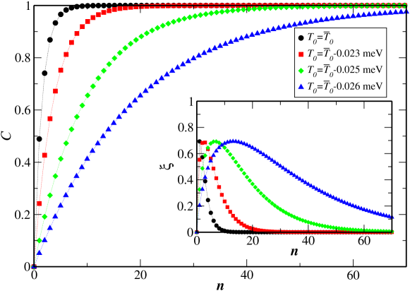
Figure 4: Dot-dot entanglement $C$ as a function of the number $n$ of the carriers injected into the device evaluated at four different values of the kinetic energy $T_{0}$ close to the resonance condition $\bar{T}_{0}$. As input condition, the bound particles occupy the ground state of the DQDs system. All the curves tend to 1 for large values of $n$. The farther is the kinetic energy of each incident electron from $\bar{T}_{0}$, the slower the asymptotic value 1 is reached. The inset displays the dependence of the DQD decoherence $\xi$ upon $n$, for the same four values of $T_{0}$.

As shown in the inset of Figure 4, we find that a series of scatterings does not induce decoherence of the DQD first-excited state even for carriers injected with kinetic energies not exactly equal but close enough to $\bar{T}_{0}$. This implies that maximally-entangled states of the DQD are produced as an effect of the flux of the charge carriers even if the energy of the incident electrons is not precisely the resonant one. Specifically, the farther $T_{0}$ is from $\bar{T}_{0}$, the larger $n$ is needed to produce a Bell state decoupled from the environment. In fact, when the initial kinetic energy of the carriers gets away from the resonant one, the parameter $p_{00}$, acting as a convergence factor, increases and the injection of more carriers in the device is needed to build up the maximum amount of quantum correlations between the dots. From the inset of Figure 4, we also note that the number $n$ of electrons needed to have a vanishing decoherence (i.e. the DQD in a pure state) is lower for $T_{0}$ closer to $\bar{T}_{0}$. In particular, $\xi$ shows a maximum, whose value is about $\ln{2}$ when the interaction with the injected carriers reduces the state of the system to a statistical mixture with equal weights of the ground $|\epsilon_{0}\rangle$ and the excited $|\epsilon_{2}\rangle$ states. This occurs for $p_{00}^{n}$=$2^{-1/n}$. As expected, the peak is at higher values of $n$ when the injection energy of the carriers is farther from $\bar{T}_{0}$ and, as a consequence, $p_{00}$ is larger.

In analogy to the case of entanglement creation described above, a current of charge carriers injected at an appropriate energy can be a means to disentangle the DQD prepared in the Bell state $|\epsilon_{2}\rangle\frac{1}{\sqrt{2}}\left(|0_{L}1_{R}\rangle+|1_{L}0_{R}\rangle\right)$. In order to show this, Figure 5 displays the disentanglement effect for electrons injected with kinetic energy $T_{0}$ around 2.6 meV and scattered by the bound particles of the DQDs.

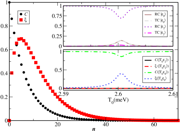
Figure 5: Dot-dot entanglement $C$ and DQD decoherence $\xi$ as a function of the number $n$ of the carriers injected into the device at the resonant kinetic energy $T_{0}$=2.6 meV. As input condition, the bound particles occupy the first-excited state $|\epsilon_{2}\rangle$ of the DQDs system corresponding to the Bell-state $\frac{1}{\sqrt{2}}\left(|0_{L}1_{R}\rangle+|1_{L}0_{R}\rangle\right)$. Both $C$ and $\xi$ vanish at large $n$. The top inset displays the modulus of the TC and RC of the channels $|\epsilon_{0}\rangle$ and $|\epsilon_{2}\rangle$ of the DQD as a function of $T_{0}$ around the resonant condition when the input state of the total system is $|T_{0}\epsilon_{2}\rangle$: RC of channel $|\epsilon_{0}\rangle$ (solid line), TC of channel $|\epsilon_{0}\rangle$ (dashed line), RC of channel $|\epsilon_{2}\rangle$ (dotted line), TC of channel $|\epsilon_{2}\rangle$ (dot-dashed line). The bottom inset shows the entanglement $C$ and the decoherence $\xi$ for the two input states $|T_{0}\epsilon_{0}\rangle$ and $|T_{0}\epsilon_{2}\rangle)$: $C(|T_{0}\epsilon_{0}\rangle)$ (solid line), $\xi(|T_{0}\epsilon_{0}\rangle)$ (dashed line), $C(|T_{0}\epsilon_{2}\rangle)$ (dash-dotted line), and $\xi(|T_{0}\epsilon_{2}\rangle)$ (dotted line). Note that the abscissa scale is the same in the top and bottom insets.

For such a low kinetic energy, the scattering by a single carrier leaves unaltered the DQDs system when the bound electrons are in the ground state $|\epsilon_{0}\rangle$. In fact $T_{0}$ is smaller than the energy necessary to excite the dots. This means that the the scattered carrier has not been coupled, via Coulomb interaction, to the bound particles, which remain maximally disentangled (see the bottom inset of the Figure 5). On the other hand, when the input state of the total system is $|T_{0}\epsilon_{2}\rangle$ the dots can relax. In fact the scattering channels corresponding to $|\epsilon_{0}\rangle$ show a peak in the transmission and reflection spectra (as shown in the top inset of Figure 5) thus leading to the appearance of decoherence and entanglement.

By applying the approach adopted above for building up maximum entanglement between the bound electrons, we find that the scattering by a current of charge carriers with energy around $T_{0}=2.6$ meV is able to disentangle completely the quantum dots without introducing any decoherence. Specifically, after a larger number $n$ of scattered carriers, the bound electrons practically occupy the ground state of the DQD system: this means $C=0$ and $\xi=0$, as reported in Figure 5.

5 Conclusions

The coherent manipulation of electron states is the key ingredient for implementing qubits using charge or orbital states of DQD nanostructures. Indeed, it implies the controlled production or destruction, the manipulation and detection of entanglement between the above states. In this spirit, various proposals to produce bipartite entangled state have been advanced on the basis of the physical mechanisms requiring two-particle scattering, such as the direct interaction between two electrons [24, 25, 23, 33, 53]. In this work, we have investigated the appearance of quantum correlations between the two electrons of a GaAs DQD, as a consequence of the Coulomb scattering by one or more charge carriers injected from a lead. We examined the scattering event in a three-particle regime (the two electrons trapped in the DQDs and the passing carrier, explicitely considered indistinguishable), that is, a carrier is supposed to enter in the scattering region only after the previous one has already left. Furthermore, the two dots are taken distant enough so that the Coulomb repulsion between the two bound electrons is practically negligible. Therefore, unlike other approaches [25, 23], the scattered carrier represents the entanglement “mediator”, that is, it provides the indirect interaction between the particles needed to entangle them. From this point of view, various scheme where entanglement between distant particles is produced though their scattering by mobile mediators are present in literature [50, 54]. Unlike our model, there the quantum correlations are built among the spin degrees of the freedom of the particles.

A proper tuning of the carrier energy and the DQD geometry reduces the system here examined to a simple two-qubit model coupled to the external degrees of freedom by the incident electrons. Here, the dots have not been considered as point-like systems [7, 17, 18, 19, 20] but their effective spatial dimensions are explicitely taken into account in the calculation. Indeed, the knowledge of the electron spatial wavefunctions corresponding to eigenstates of the DQD is needed to obtain the few-particle scattering states. To this aim, a time-independent approach based on the QTBM has been used [21, 22, 23]. Its solution gives the reflection and transmission amplitude of each scattering channel as a function of the initial energy of the incoming electron. Such an approach permits to analyze the relation between the resonances in the transmission and reflection spectra and the appearance of quantum correlations between the particles, as already pointed out elsewhere [25, 23, 26]. All the travelling components of the scattered carrier, both reflected and transmitted, have been used to evaluate the creation of the entanglement between the dots, together with their decoherence.

Our numerical simulations show that as a consequence of the scattering between an electron injected with a suitable energy and two electrons bound in the ground state of the DQD system, the latter can be excited, ending up in an entangled state of the constituent dots. This process leads to the appearance of resonance peaks and dips in transmission and reflection spectra of the first-excited and ground scattering channels, respectively. A side-effect of such a scattering is the loss of quantum coherence of the DQD as whole due to its coupling to the scattered carrier. The condition of maximum entanglement between the two dots is reached when the bound electrons are fully raised to the two-particle first-excited level of the DQD system (which corresponds to a Bell-state formed with the single-particle ground and first-excited states of the two dots). In this case, the DQD decoherence is zero, since a single output channel is possible. However, a single collision is not able to fully excite the dots. We found that, in order to build up the maximum amount of quantum correlation between them, a repeated injection of charge carriers, that is an electric current, is needed. Indeed, at each scattering event the excitation probability of the dots increases until it reaches asymptotically 1, which means that a Bell state is obtained, fully decoupled from the degrees of freedom of the scattered carriers. In other words, the Coulomb interaction between an electric current and two electrons bound in the ground state of a DQD structure allows for the maximum entanglement production while the decoherence effects on the system vanish. This is in agreement with the procedures adopted in other works [26, 47, 48, 49, 50], where the entangling schemes are based on the successive interactions of a mediator with the qubits. However, in our scheme, the indirect coupling of the two dots due to interaction with the scattered carriers, can produce disentangling effects, as well. Indeed, a proper tuning of the electric current makes the DQD, initially in a Bell state to relax into the ground state, with no quantum correlations. Also in this case the process results to be robust against decoherence.

Finally, the results here reported show how a suitable electron current, where all the carriers have almost a given kinetic energy, permits to switch coherently on and off the entanglement between the dots of a DQD structure. Although several interaction mechanisms, as electron-phonon coupling can lead to the loss of quantum coherence of the DQD in a real experimental setup, we showed that interaction with the mediator electrons does not generate entanglement with the leads. Thus, no intrinsic decoherence is implied.

Appendix A Evaluation of the reduced density matrix $\rho_{r}^{(n)}$

Here we shall give the explicit derivation of the reduced density matrix of the two dots (see equation (17)), initially taken in their ground state, once $n$ carriers injected with kinetic energy $T_{0}$ close to $\bar{T_{0}}$ have been scattered. In order to simplify the calculation, the basis $\mathcal{C}=\{|\epsilon_{0}\rangle,|\epsilon_{1}\rangle,|\epsilon_{2}\rangle,|\epsilon_{3}\rangle\}$ of the DQD eigenstates will be used. Once obtained the reduced density operator ${\rho_{r}^{(n)}}^{\prime}$ in the $\mathcal{C}$ basis, its expression ${\rho_{r}^{(n)}}$ in terms of the $\mathcal{B}$ is straightforward (see Table 1).

The output three-particle state of equation (16), stemming from the scattering between one carrier injected in the device with $T_{0}$=$\bar{T_{0}}$ and the two electrons in the ground state of the DQD, can be written as

$$|{\Psi_{OUT}^{(1)}}^{\prime}\rangle=\left(\tilde{b}_{00}|{T^{<}_{0}}^{(1)}\rangle+\tilde{c}_{00}|{T^{>}_{0}}^{(1)}\rangle\right)|\epsilon_{0}\rangle+\left(\tilde{b}_{02}|{T^{<}_{-2}}^{(1)}\rangle+\tilde{c}_{02}|{T^{>}_{-2}}^{(1)}\rangle\right)|\epsilon_{2}\rangle,$$ (19)

where the superscript (1) means 1 carrier injected, and the reduced density matrix of the DQD system can be obtained by tracing $|{\Psi_{OUT}^{(1)}}^{\prime}\rangle\langle{\Psi_{OUT}^{(1)}}^{\prime}|$ over the degrees of freedom ${T^{>(<)}_{i}}^{(1)}$ of the scattered carrier

$${\rho_{r}^{(1)}}^{\prime}=\left(\begin{array}[]{cccc}p_{00}&0&0&0\\ 0&0&0&0\\ 0&0&1-p_{00}&0\\ 0&0&0&0\end{array}\right).$$ (20)

When a second carrier is injected, after the exit of the previous one from the scattering region, the new output state is

$$|{\Psi^{(2)}_{OUT}}^{\prime}\rangle=\left(\tilde{b}_{00}|{T^{<}_{0}}^{(2)}\rangle+\tilde{c}_{00}|{T^{>}_{0}}^{(2)}\rangle\right)\left(\tilde{b}_{00}|{T^{<}_{0}}^{(1)}\rangle+\tilde{c}_{00}|{T^{>}_{0}}^{(1)}\rangle\right)|\epsilon_{0}\rangle+$$

$$\left(\tilde{b}_{02}|{T^{<}_{-2}}^{(2)}\rangle+\tilde{c}_{02}|{T^{>}_{-2}}^{(2)}\rangle\right)\left(\tilde{b}_{00}|{T^{<}_{0}}^{(1)}\rangle+\tilde{c}_{00}|{T^{>}_{0}}^{(1)}\rangle\right)|\epsilon_{2}\rangle+$$

$$\left(\tilde{b}_{22}|{T^{<}_{0}}^{(2)}\rangle+\tilde{c}_{22}|{T^{>}_{0}}^{(2)}\rangle\right)\left(\tilde{b}_{02}|{T^{<}_{-2}}^{(1)}\rangle+\tilde{c}_{02}|{T^{>}_{-2}}^{(1)}\rangle\right)|\epsilon_{2}\rangle.$$ (21)

As stressed in Section 4, when the DQD is in $|\epsilon_{2}\rangle$, the scattering event does not produce the relaxation of the dots which remain in the excited energy level. This means that in the above expression $|\tilde{b}_{22}|^{2}+|\tilde{c}_{22}|^{2}=1$. The reduced density matrix of the DQD computed from the three-particle state of equation (A) is

$${\rho_{r}^{(2)}}^{\prime}=\left(\begin{array}[]{cccc}p_{00}^{2}&0&0&0\\ 0&0&0&0\\ 0&0&(1-p_{00}^{2})&0\\ 0&0&0&0\end{array}\right),$$ (22)

where $p_{00}$=$|\tilde{b}_{00}|^{2}+|\tilde{c}_{00}|^{2}$=$1-|\tilde{b}_{02}|^{2}-|\tilde{c}_{02}|^{2}$ have been used. For the case of $n$ scattered particles we get

$${\rho_{r}^{(n)}}^{\prime}=\left(\begin{array}[]{cccc}p_{00}^{n}&0&0&0\\ 0&0&0&0\\ 0&0&(1-p_{00}^{n})&0\\ 0&0&0&0\end{array}\right),$$ (23)

as derived by induction in the following. Assume that expression (23) is true for $n$. This implies that ${\rho_{r}^{(n)}}^{\prime}=p_{00}^{n}|\epsilon_{0}\rangle\langle\epsilon_{0}|+(1-p_{00}^{n})|\epsilon_{2}\rangle\langle\epsilon_{2}|$. After the injection of the $(n+1)$-th carrier, the density matrix $\rho^{\prime}(\epsilon_{i},\epsilon_{j},{T^{<(>)}_{l}}^{(n+1)},{T^{<(>)}_{m}}^{(n+1)})$ describing the total system can be evaluated from ${\rho_{r}^{(n)}}^{\prime}$:

$$\rho^{\prime}(\epsilon_{i},\epsilon_{j},{T^{<(>)}_{j}}^{(n+1)},{T^{<(>)}_{m}}^{(n+1)})=$$

$$p_{00}^{n}\bigg{[}\left(\tilde{b}_{00}|{T^{<}_{0}}^{(n+1)}\rangle+\tilde{c}_{00}|{T^{>}_{0}}^{(n+1)}\rangle\right)|\epsilon_{0}\rangle\langle\epsilon_{0}|\left(\tilde{b}_{00}^{\ast}\langle{T^{<}_{0}}^{(n+1)}|+\tilde{c}_{00}^{\ast}\langle{T^{>}_{0}}^{(n+1)}|\right)+$$

$$\left(\tilde{b}_{00}|{T^{<}_{0}}^{(n+1)}\rangle+\tilde{c}_{00}|{T^{>}_{0}}^{(n+1)}\rangle\right)|\epsilon_{0}\rangle\langle\epsilon_{2}|\left(\tilde{b}_{02}^{\ast}\langle{T^{<}_{-2}}^{(n+1)}|+\tilde{c}_{02}^{\ast}\langle{T^{>}_{-2}}^{(n+1)}|\right)+$$

$$\left(\tilde{b}_{02}|{T^{<}_{-2}}^{(n+1)}\rangle+\tilde{c}_{02}|{T^{>}_{-2}}^{(n+1)}\rangle\right)|\epsilon_{2}\rangle\langle\epsilon_{0}|\left(\tilde{b}_{00}^{\ast}\langle{T^{<}_{0}}^{(n+1)}|+\tilde{c}_{00}^{\ast}\langle{T^{>}_{0}}^{(n+1)}|\right)+$$

$$\left(\tilde{b}_{02}|{T^{<}_{-2}}^{(n+1)}\rangle+\tilde{c}_{02}|{T^{>}_{-2}}^{(n+1)}\rangle\right)|\epsilon_{2}\rangle\langle\epsilon_{2}|\left(\tilde{b}_{02}^{\ast}\langle{T^{<}_{-2}}^{(n+1)}|+\tilde{c}_{02}^{\ast}\langle{T^{>}_{-2}}^{(n+1)}|\right)\bigg{]}+$$

$$(1-p_{00}^{n})\left(\tilde{b}_{22}|{T^{<}_{0}}^{(n+1)}\rangle+\tilde{c}_{22}|{T^{>}_{0}}^{(n+1)}\rangle\right)|\epsilon_{2}\rangle\langle\epsilon_{2}|\left(\tilde{b}_{22}^{\ast}\langle{T^{<}_{0}}^{(n+1)}|+\tilde{c}_{22}^{\ast}\langle{T^{>}_{0}}^{(n+1)}|\right).$$ (24)

By tracing $\rho^{\prime}(\epsilon_{i},\epsilon_{j},{T^{<(>)}_{j}}^{(n+1)},{T^{<(>)}_{m}}^{(n+1)})$ over the degrees of freedom ${T^{<(>)}_{j}}^{(n+1)}$ of the carrier, one obtains the reduced density matrix ${\rho_{r}^{(n+1)}}^{\prime}$ of the DQD scattered by $n+1$ electrons. Its expression reads

$${\rho_{r}^{(n+1)}}^{\prime}=p_{00}^{n}\bigg{(}|b_{00}|^{2}+|c_{00}|^{2}\bigg{)}|\epsilon_{0}\rangle\langle\epsilon_{0}|+\bigg{(}p_{00}^{n}(|b_{02}|^{2}+|c_{02}|^{2})+(1-p_{00}^{n})(|b_{22}|^{2}+|c_{22}|^{2})\bigg{)}|\epsilon_{2}\rangle\langle\epsilon_{2}|=$$

$$p_{00}^{n+1}|\epsilon_{0}\rangle\langle\epsilon_{0}|+(1-p_{00}^{n+1})|\epsilon_{2}\rangle\langle\epsilon_{2}|.$$ (25)

Thus the expression (23) is true for $n+1$.

Finally, the unitary transformation of Table 1 can be applied to ${\rho_{r}^{(n)}}^{\prime}$ in order to obtain the reduced density matrix of the two electrons bound in the DQD given in equation (17).

References

References

- [1] Kane B 1998 Nature 393 133
- [2] Nakamura Y, Pashkin Y and Tsai J 1999 Nature 398 786
- [3] Loss D and DiVincenzo D P 1998 Phys. Rev. A 57 120
- [4] Fedichkin L, Yanchenko M and Valiev K A 2000 Nanotechnology 11 387
- [5] DiVincenzo D, Bacon D, Kempe J, Burkard G and Whaley K 2000 Nature 408 339
- [6] Brandes T and Vorrath T 2002 Phys. Rev. B 66 075341
- [7] Wu Z J, Zhu K D, Yuan X Z, Jiang Y W and Zheng H 2005 Phys. Rev. B 71 205323
- [8] van der Wiel W G, De Franceschi S, Elzerman J M, Fujisawa T, Tarucha S and Kouwenhoven L P 2002 Rev. Mod. Phys. 75 1–22
- [9] van Wees B J, van Houten H, Beenakker C W J, Williamson J G, Kouwenhoven L P, van der Marel D and Foxon C T 1988 Phys. Rev. Lett. 60 848–850
- [10] Meirav U, Kastner M A and Wind S J 1990 Phys. Rev. Lett. 65 771–774
- [11] Lassen B and Wacker A 2007 Phys. Rev. B 76 075316
- [12] DiVincenzo D, Burkard G, Loss D and Sukhorukov E 2000 Quantum Mesoscopic Phenomena and Mesoscopic Devices (Dordrecht: Kluwer Academic Publishers)
- [13] Hayashi T, Fujisawa T, Cheong H D, Jeong Y H and Hirayama Y 2003 Phys. Rev. Lett. 91 226804
- [14] Petta J R, Johnson A C, Marcus C M, Hanson M P and Gossard A C 2004 Phys. Rev. Lett. 93 186802
- [15] Shinkai G, Hayashi T, Ota T and Fujisawa T 2009 Phys. Rev. Lett. 103 056802
- [16] Stavrou V N and Hu X 2005 Phys. Rev. B 72 075362
- [17] Vorojtsov S, Mucciolo E R and Baranger H U 2005 Phys. Rev. B 71 205322
- [18] Cao X and Zheng H 2007 Phys. Rev. B 76 115301
- [19] Openov L 2008 Physics Letters A 372 3476
- [20] Li Z Z, Pan X Y and Liang X T 2008 Physica E 41 220
- [21] Lent C S and Kirkner D J 1990 Journal of Applied Physics 67 6353
- [22] Bertoni A and Goldoni G 2007 Phys. Rev. B 75 235318
- [23] Buscemi F, Bordone P and Bertoni A 2007 Phys. Rev. B 76 195317
- [24] Oliver W D, Yamaguchi F and Yamamoto Y 2002 Phys. Rev. Lett. 88 037901
- [25] López A, Rendón O, Villaba V M and Medina E 2007 Phys. Rev. B 75 033401
- [26] Yuasa K and Nakazato H 2007 Journal of Physics A: Mathematical and Theoretical 40 297
- [27] Ciccarello F, Paternostro M, Palma G M and Zarcone M 2009 New Journal of Physics 11 113053
- [28] Fogler M M 2005 Phys. Rev. Lett. 94 056405
- [29] Stavrou V N and Hu X 2006 Phys. Rev. B 73 205313
- [30] Bertoni A, Rontani M, Goldoni G and Molinari E 2005 Phys. Rev. Lett. 95 066806
- [31] Schliemann J, Cirac J I, Kuś M, Lewenstein M and Loss D 2001 Phys. Rev. A 64 022303
- [32] Ghirardi G and Marinatto L 2004 Phys. Rev. A 70 012109
- [33] Buscemi F, Bordone P and Bertoni A 2006 Phys. Rev. A 73 052312
- [34] Eckert K, Schliemann J, Bruß D and Lewenstein M 2002 Annals of Physics 299 88
- [35] Peres A 1995 Quantum theory: concepts and methods (Dordrecht: Kluwer Academic Publishers)
- [36] Wootters W K 1998 Phys. Rev. Lett. 80 2245–2248
- [37] Bellomo B, Lo Franco R and Compagno G 2007 Phys. Rev. Lett. 99 160502
- [38] Yu T and Eberly J 2007 Quantum Inf. Comp. 7 459
- [39] Breit G and Wigner E 1936 Phys. Rev. 49 519–531
- [40] Fano U 1961 Phys. Rev. 124 1866–1878
- [41] Hao X, Li J, Lv X Y, Si L G and Yang X 2009 Physics Letters A 373 3827
- [42] Habgood M, Jefferson J H, Ramšak A, Pettifor D G and Briggs G A D 2008 Phys. Rev. B 77 075337
- [43] Zurek W H 1982 Phys. Rev. D 26 1862
- [44] Duan L M and Guo G C 1998 Phys. Rev. A 57 737
- [45] Zanardi P and Rasetti M 1997 Phys. Rev. Lett. 79 3306
- [46] Patra M K and Brooke P G 2008 Phys. Rev. A 78 010308
- [47] Browne D E and Plenio M B 2003 Phys. Rev. A 67 012325
- [48] Compagno G, Messina A, Nakazato H, Napoli A, Unoki M and Yuasa K 2004 Phys. Rev. A 70 052316
- [49] Migliore R, Yuasa K, Nakazato H and Messina A 2006 Phys. Rev. B 74 104503
- [50] Costa A T, Bose S and Omar Y 2006 Phys. Rev. Lett. 96 230501
- [51] Bjork M, Ohlsson B, Thelander C, Persson AIand Deppert K and Wallenberg LRand Samuelson L 2002 Applied Physics Letters 81 4458–4460
- [52] Feve G, Mahe A, Berroir J-Mand Kontos T, Plaçais B, Glattli D, Cavanna A, Etienne B and Jin Y 2007 Science 316 1169–1172
- [53] Schomerus H and Robinson J P 2007 New Journal of Physics 9 67
- [54] Ciccarello F, Palma G M, Zarcone M, Omar Y and Vieira V R 2006 New Journal of Physics 8 214