On the One dimensional Poisson Random Geometric Graph

Abstract.

Given a Poisson process on a bounded interval, its random geometric graph is the graph whose vertices are the points of the Poisson process and edges exist between two points if and only if their distance is less than a fixed given threshold. We compute explicitly the distribution of the number of connected components of this graph. The proof relies on inverting some Laplace transforms.

1. Motivation

As technology goes on [1, 2, 3], one can expect a wide expansion of the so-called sensor networks. Such networks represent the next evolutionary step in building, utilities, industrial, home, agriculture, defense and many other contexts [4].

These networks are built upon a multitude of small and cheap sensors which are devices with limited transmission capabilities. Each sensor monitors a region around itself by measuring some environmental quantities (e.g., temperature, humidity), detecting intrusion, etc, and broadcasts its collected informations to other sensors or to a central node. The question of whether information can be shared among the whole network is then of crucial importance.

Many researches have recently been dedicated to this problem considering a variety of situations. It is possible to categorize three main scenarios: those where it is possible to choose the position of each sensor, those where sensors are arbitrarily deployed in the target region with the control of a central station and those where the sensor locations are random in a decentralized system.

The problem of the first scenario is that, in many cases, placing the sensors is impossible or implies a high cost. Sometimes this impossibility comes from the fact that the cost of placing each sensor is too large and sometimes the network has an inherent random behavior (like in the ad hoc case, where users move). In addition, this policy cannot take into account the configuration of the network in the case of failure of some sensor.

The drawback of the second scenario is a higher unity cost of sensors, since each one has to communicate with the central station. Besides, the central station itself increases the cost of the whole system. Moreover, if sensors are supposed to know their positions, an absolute positioning system has to be included in each sensor, making their hardware even more complex and then more expensive.

It is thus important to investigate the third scenario: randomly located sensors, no central station. Actually, if we can predict some characteristics of the topology of a random network, the number of sensors (or, as well, the power supply of them) can be a priori determined such that a given network may operate with high probability. For instance, we can choose the mean number of sensors such that, if they are randomly deployed, there is more than 99% of probability the network to be completely connected.

Usually, sensors are deployed in the plane or in the ambient space, thus mathematically speaking, one has to deal with configurations in ${\mathbf{R}}^{2},$ ${\mathbf{R}}^{3}$ or a manifold. The recent works of Ghrist and his collaborators [5, 6] show how, in any dimension, algebraic topology can be used to compute the coverage of a given configuration of sensors. Trying to pursue their work for random settings, we quickly realized that the dimension of the ambient space played a key role. We then first began by the analysis of dimension $1$, which appeared as the most simple situation. There is here no need of the sophisticated tools of algebraic topology. However, it doesn’t seem that the problem of coverage on a finite length interval has already been solved in the full extent we do here. Higher dimensions will be the object of forthcoming papers.

We here address the situation where the radio communications are sufficently polarized so that we can consider we have some privileged dimension. Random coverage in one dimension has been already studied in different contexts. Some years ago already, several analysis were done on the circle ([7, 8] and references therein) for a fixed number of points and uniform distribution of points over the circle. The question addressed was that of full coverage. More recently, in [9], efficient algorithms to determine whether a region is covered considering the sensors are deployed over a circle and distributed as a Poisson point process are given. In [7, 10], the distribution of a fixed number of clusters (see below for the definition) is given. In [11], sensors are actually placed in a plan, have a fixed radius of observation. The trace of the covered regions over a line is then studied.

Our main result is the distribution of the number of connected components for a Poisson distribution of sensors in a bounded interval. Our method is very much related to queueing theory. Indeed, clusters, i.e., sequence of neighboring sensors, are the strict analogous of busy periods. As will appear below, our analysis turns down to be that of an M/D/1/1 queue with preemption: when a customer arrives during a service, it preempts the server and, since there is no buffer, the customer who was in service is removed from the queuing system. To the best of our knowledge, such a system has never been studied but the usual methods of Laplace transform, renewal processes, work perfectly and with a bit of calculus, one can compute all the characteristics we are interested in.

The paper is organized in the following way: Section II presents the physical and random assumptions and defines the relevant quantities to be calculated. The calculations and analytical results are presented in Section III. In section IV, two other scenarios are presented, considering the number of incomplete clusters and clusters placed in a circle. In Section V, numerical examples are presented and analyzed.

2. Problem Formulation

Let $L>0$ be the length of the domain in which sensors are located. We assume that sensors are distributed according to a Poisson process of intensity $\lambda$. Let $(X_{i},\,1\leq i\leq n)$ be the positions of the sensors. We thus know that the random variables, $\Delta X_{i}=X_{i+1}-X_{i}$ are i.i.d. and exponentially distributed. Due to their technological limitations, each sensor can communicate only with other sensors within a range $\epsilon$: two sensors, located respectively at $x$ and $y$, are said to be directly connected whenever $|x-y|\leq\epsilon.$ For $i<j$, two sensors located at $X_{i}$ and $X_{j}$ are indirectly connected if $X_{l}$ and $X_{l+1}$ are directly connected for any $l=i,\,\cdots,\,j-1.$ A set of sensors directly or indirectly connected is called a cluster and the connectivity of the whole network is measured by the number of clusters.

The number of points in the interval $[0,x]$ is denoted by $N_{x}=\sum_{n=0}^{\infty}{\mathbf{1}}_{\left\{{X_{n}\leq x}\right\}}$. The random variable $A_{i}$ given by

$$A_{i}=\left\{\begin{array}[]{ll}X_{1}&\mbox{ if }i=1,\\ \mbox{inf}_{j}\{X_{j}|X_{j}>A_{i-1},X_{j}-X_{j-1}>\epsilon\}&\mbox{ if }i>1,\end{array}\right.$$

represents the beginning of the $i$-th cluster, denoted by $C_{i}$. In the same way, the end of this same cluster, $E_{i}$, is defined by

$$E_{i}=\mbox{inf}_{j}\{X_{j}+\epsilon|X_{j}>A_{i},X_{j+1}-X_{j}>\epsilon\}.$$

So, the $i$-th cluster, $C_{i}$, has a number of points given by $N_{E_{i}}-N_{A_{i}}$. We define the length $B_{i}$ of $C_{i}$ as $E_{i}-A_{i}$. The intercluster size, $D_{i}$, is the distance between the end of $C_{i}$ and the beginning of $C_{i+1}$, which means that $D_{i}=A_{i+1}-E_{i}$ and $\Delta A_{i}$ is the distance between the first points of two consecutive clusters $C_{i}$, given by $\Delta A_{i}=A_{i+1}-A_{i}=B_{i}+D_{i}$.

Remark 1.

With this set of assumptions and definitions, we can see our problem actually as an $M/D/1/1$ preemptive queue, Fig. 1. In this non-conservative system, the service time is deterministic and given by $\epsilon$. When a customer arrives during a service, the served customer is removed from the system and replaced by the arriving customer. Within this framework, a cluster corresponds to what is called a busy period, the intercluster size is the idle time and $A_{i}+D_{i}$ is the length of the $i$-th cycle.

Figure 1. Queueing representation of the proposed problem. A down arrow denotes that user $i$ starts to be served. An up arrow indicates that user $i$ leaves the system without have finished the service. A double up arrow illustrates that the service of user $i$ finishes. It is also shown the beginning and the end of the $i$th busy period, respectively, $A_{i}$ and $E_{i}$.

The number of complete clusters in $[0,L]$ corresponds to the number of connected components $\beta_{0}(L)$ (since in dimension $1$, it coincides with the Euler characteristics of the union of intervals, see [12, 5]) of the network. The distance between the beginning of the first cluster and the beginning of the $(i+1)$-th one is defined as $U_{i}=\sum_{k=1}^{i}\Delta A_{k}$. We also define $\Delta X_{0}=D_{0}=X_{1}$. Fig. 2 illustrates these definitions.

Figure 2. Definitions of the relevant quantities of the network: distance between points, distance between clusters, the size of clusters, the size interclusters, the beginning of clusters and the end of clusters.

Lemma 1.

For any $i\in\mathbb{N}_{+}^{*}$, $A_{i}$ and $E_{i}$ are stopping times.

Proof.

Let us consider the filtration $\mathcal{F}_{t}=\sigma\{N_{a},a\leq t\}$. For $i=1$, we have

$$\{A_{1}\leq t\}\Leftrightarrow\{X_{1}\leq t\}\Leftrightarrow\{N_{t}\geq 1\}\in\mathcal{F}_{t}.$$

Thus, $A_{1}$ is a stopping time. For $A_{2}$, we have

$$\{A_{2}>t\}\Leftrightarrow\bigcup_{n\geq 1}\left\{N_{t}=n,\bigcup_{j=1}^{n}\left\{\Delta X_{j}\geq\epsilon,\bigcup_{k=j+1}^{n}\{\Delta X_{k}\leq\epsilon\}\right\}\right\}\in\mathcal{F}_{t},$$

so $A_{2}$ is also a stopping time. We proceed along the same line for others $A_{i}$ and as well for $E_{i}$ to prove that they are stopping times. ∎

Since $N$ is a strong Markov process, the next corollary is immediate.

Corollary 2.

The set $\{B_{i},D_{i}\,|\,i=\geq 1\}$ is a set of independent random variables. Moreover, $D_{i}$ is distributed as an exponential random variable with mean $1/\lambda$ and the random variables $\{B_{i}\,|\,i\geq 1\}$ are i.i.d.

3. Calculations

Theorem 3.

The Laplace transform of the distribution of $B_{i}$, is given by

$$\mathbb{E}\left[e^{-sB_{i}}\right]=\frac{\lambda+s}{\lambda+se^{(\lambda+s)\epsilon}}\cdotp$$

Proof.

Since $\Delta X_{j}$ is an exponentially distributed random variable,

$$\mathbb{E}\left[e^{-s\Delta X_{j}}{\mathbf{1}}_{\left\{{\Delta X_{j}\leq\epsilon}\right\}}\right]=\int_{0}^{\epsilon}e^{-st}\lambda e^{-\lambda t}dt=\frac{\lambda}{s+\lambda}\left(1-e^{-(s+\lambda)\epsilon}\right).$$

Hence, the Laplace transform of the distribution of $B_{1}$ is given by

$$\mathbb{E}\left[e^{-sB_{1}}\right] =\sum_{n=1}^{\infty}\mathbb{E}\left[e^{-sB_{1}},N_{E_{1}}=n\right]$$

$$=\sum_{n=1}^{\infty}\mathbb{E}\left[e^{-s(\sum_{j=1}^{n-1}\Delta X_{j}+\epsilon)}{\mathbf{1}}_{\left\{{\Delta X_{n}>\epsilon}\right\}}\prod_{j=1}^{n-1}{\mathbf{1}}_{\left\{{\Delta X_{j}\leq\epsilon}\right\}}\right]$$

$$=\sum_{n=1}^{\infty}\left(\mathbb{E}\left[e^{-s\Delta X_{1}}{\mathbf{1}}_{\left\{{\Delta X_{1}\leq\epsilon}\right\}}\right]\right)^{n-1}\mathbb{E}\left[e^{-s\Delta X_{n}}{\mathbf{1}}_{\left\{{\Delta X_{n}>\epsilon}\right\}}\right]e^{-s\epsilon}$$

$$=\sum_{n=0}^{\infty}\left(\frac{\lambda}{s+\lambda}(1-e^{-(s+\lambda)\epsilon})\right)^{n}e^{-s\lambda}e^{-s\epsilon}$$

$$=\frac{\lambda+s}{se^{\lambda\epsilon}e^{s\epsilon}+\lambda},$$

Using Collorary 2, we have $\mathbb{E}\left[e^{-sB_{1}}\right]=\mathbb{E}\left[e^{-sB_{i}}\right]$, which concludes the proof. ∎

From this result, we can immediately calculate the Laplace transform of the distribution of $\Delta A_{i}$. Since $\Delta A_{i}=B_{i}+D_{i}$, we have $\mathbb{E}\left[e^{-s\Delta A_{i}}\right]=\mathbb{E}\left[e^{-s(B_{i}+D_{i})}\right]$ and using Corollary 2:

$$\mathbb{E}\left[e^{-s\Delta A_{i}}\right]=\mathbb{E}\left[e^{-sB_{i}}\right]\mathbb{E}\left[e^{-sD_{i}}\right]=\frac{\lambda}{\lambda+se^{(\lambda+s)\epsilon}}\cdotp$$

Corollary 4.

The Laplace transform of the distribution of $U_{n}$, for $n\geq 0$ is given by

$$\mathbb{E}\left[e^{-sU_{n}}\right]=\frac{\lambda^{n}}{\left(\lambda+se^{(\lambda+s)\epsilon}\right)^{n}}\cdotp$$

Proof.

We use Corollaries 2 and 3 to calculate the Laplace transform of the distribution of $U_{n}$, since $U_{n}=\sum_{i=1}^{n}(B_{i}+D_{i})$:

$$\mathbb{E}\left[e^{-sU_{n}}\right] =\prod_{i=1}^{n}\mathbb{E}\left[e^{-sB_{i}}\right]\mathbb{E}\left[e^{-sD_{i}}\right]$$

$$=\left(\frac{\lambda+s}{\lambda+se^{(\lambda+s)\epsilon}}\right)^{n}\left(\frac{\lambda}{\lambda+s}\right)^{n},$$

hence the result. ∎

Let us define the function $p_{n}$ as

$$p_{n}\,:\,x\in{\mathbf{R}}^{+}\longmapsto p_{n}(x)=\Pr(\beta_{0}(x)=n),$$

i.e., $p_{n}(x)$ is the probability of having $n$ clusters in the interval $[0,\,x]$. Since for all $x\in{\mathbf{R}}_{+}$, $0\leq p_{n}(x)\leq 1$, the Laplace transform of $p_{n}$ with respect to $x$,

$$\mathcal{L}\{p_{n}\}(s)=\int_{0}^{\infty}e^{-sx}p_{n}(x){\text{ d}}x,$$

is well defined.

Theorem 5.

For any $n\geq 0$, the Laplace transform of $p_{n}$ is given by

(2) $$\mathcal{L}\{p_{n}\}(s)=\frac{\lambda^{n}\,e^{(\lambda+s)\epsilon}}{\left(se^{(\lambda+s)\epsilon}+\lambda\right)^{n}}\cdotp$$

Proof.

We note that, see Figure 3,

$$\{\beta_{0}(x)\geq n\}\Longleftrightarrow\begin{cases}\{\Delta X_{0}+U_{n-1}+B_{n}\leq L\}&\text{if }n\geq 1,\\ \{\Delta X_{0}<\infty\}&\text{if }n=0.\end{cases}$$

Figure 3. Illustration of the condition equivalent to $\beta_{0}\geq n$.

Hence

$$\Pr(\beta_{0}(x)=0)=1-\Pr(\Delta X_{0}+B_{1}\leq x),$$

and

(3) $$\Pr(\beta_{0}(x)=n)=\Pr(\Delta X_{0}+U_{n-1}+B_{n}\leq x)-\Pr(\Delta X_{0}+U_{n}+B_{n+1}\leq x).$$

Let

$$Y_{n}=\left\{\begin{array}[]{ll}\Delta X_{0}+U_{n-1}+B_{n}&\mbox{if }n\geq 1\\ 0&\mbox{if }n=0\end{array}\right.,$$

then we have:

$$\mathcal{L}\{\Pr(Y_{n}\leq\cdot)\}(s) =\int_{0}^{\infty}\Pr(Y_{n}\leq x)e^{-sx}dx$$

$$=\int_{0}^{\infty}\int_{0}^{x}dP_{Y_{n}}(y)e^{-sx}dx$$

$$=\frac{1}{s}\mathbb{E}\left[e^{-sY_{n}}\right]$$

$$=\frac{1}{s}\mathbb{E}\left[e^{-s\Delta X_{0}}\right]\mathbb{E}\left[e^{-sU_{n-1}}\right]\mathbb{E}\left[e^{-sB_{n}}\right]$$

(5) $$=\frac{1}{s}\frac{\lambda^{n}}{\left(e^{\lambda\epsilon}se^{s\epsilon}+\lambda\right)^{n}},$$

for $n\geq 1$, where we used Corollary 2 in the third line. For $n=0$, the Laplace transform is trivial and given by $\mathcal{L}\{\Pr(Y_{0}\leq\cdot)\}(s)=1/s$. Substituting Eq. (5) in the Laplace transform of both sides of Eq. (3) yields:

$$\mathcal{L}\{p_{n}\}(s) = \mathcal{L}\{\Pr(Y_{n}\leq\cdot)\}(s)-\mathcal{L}\{\Pr(Y_{n+1}\leq\cdot)\}(s)$$

$$= \frac{e^{\epsilon\lambda}e^{\epsilon s}\lambda^{n}}{\left(e^{\epsilon\lambda}se^{\epsilon s}+\lambda\right)^{n+1}},\ \ n\geq 0.$$

The proof is thus complete. ∎

Lemma 6.

Let $m$ be an positive integer. For any $x>0$, when $\epsilon\rightarrow 0$, $\mathbb{E}\left[\beta_{0}^{m}\right]\rightarrow\mathbb{E}\left[N_{L}^{m}\right]$.

Proof.

Since there is almost surely a finite number of points in $[0,\,x]$, for almost all sample-paths, there exists $\eta>0$ such that $\Delta X_{j}\geq\eta$ for any $j=1,\,\cdots,\ N_{x}$. Hence for $\epsilon<\eta$, $\beta_{0}(x)=N_{x}$. This implies that $\beta_{0}(x)$ tends almost surely to $N_{x}$ as $\epsilon$ goes to $0$. Moreover, it is immediate by the very definition of $\beta_{0}(x)$ that $\beta_{0}(x)\leq N_{x}$. Since for any $m$, $\mathbb{E}\left[N_{x}^{m}\right]$ is finite, the proof follows by dominated convergence. ∎

Let $\mbox{Li}_{t}(z)$, $z,t\in{\mathbf{R}}$, $z<1$, be the polylogarithm function with parameter $t$, defined by

$$\mbox{Li}_{t}(z)=\sum_{k=1}^{\infty}\frac{z^{k}}{k^{t}}\cdotp$$

For $m$ a positive integer, consider the function of $x$

(6) $$M_{\beta_{0}}^{m}\,:\,x\longmapsto\mathbb{E}\left[\beta_{0}^{m}(x)\right]=\sum_{i=0}^{\infty}i^{m}p_{i}(x).$$

Its Laplace transform is given by:

$$\mathcal{L}\left\{M_{\beta_{0}}^{m}\right\}(s)=\int_{0}^{\infty}\mathbb{E}\left[\beta_{0}(x)^{m}\right]e^{-sL}\,dx.$$

Corollary 7.

Let $\alpha$ be defined as follows:

$$\alpha=\frac{e^{\epsilon\lambda}}{\lambda}se^{\epsilon s}.$$

The Laplace transform of the $m$-th moment of $\beta_{0}(L)$ is:

(7) $$\mathcal{L}\left\{M_{\beta_{0}}^{m}\right\}(s)=\frac{\alpha}{s\left(\alpha+1\right)}\mbox{Li}_{-m}\left(\frac{1}{\alpha+1}\right),$$

which converges, provided that $\alpha>0.$

Proof.

Applying the Laplace transform of both sides of Eq. (6), we get:

$$\mathcal{L}\left\{M_{\beta_{0}}^{m}\right\}(s) =\sum_{i=1}^{\infty}i^{m}\mathcal{L}\{p_{i}\}(s)$$

$$=\frac{\frac{e^{\epsilon\lambda}}{\lambda}e^{\epsilon s}}{\left(\frac{e^{\epsilon\lambda}}{\lambda}se^{\epsilon s}+1\right)}\sum_{i=1}^{\infty}\frac{i^{m}}{\left(\frac{e^{\epsilon\lambda}}{\lambda}se^{\epsilon s}+1\right)^{i}}$$

$$=\frac{\alpha}{s\left(\alpha+1\right)}\mbox{Li}_{-m}\left(\frac{1}{\alpha+1}\right),$$

concluding the proof. ∎

We define $\tiny{\left\{\mbox{}\begin{array}[]{c}m\\ k\end{array}\mbox{}\right\}}$ as the Stirling number of second kind [13], i.e., $\tiny{\left\{\mbox{}\begin{array}[]{c}m\\ k\end{array}\mbox{}\right\}}$ is the number of ways to partition a set of $m$ objects into $k$ groups. They are intimately related to polylogarithm by the following identity (see [14]) valid for any positive integer $m,$

(8) $$\mbox{Li}_{-m}(z)=\sum_{k=0}^{m}\frac{(-1)^{m+k}k!\left\{\mbox{}\begin{array}[]{c}m+1\\ k+1\end{array}\mbox{}\right\}}{(1-z)^{k+1}}\cdotp$$

Corollary 8.

The $m$-th moment of the number of clusters on the interval $[0,L]$ is given by:

(11) $$M_{\beta_{0}}^{m}(L)=\sum_{k=1}^{m}\left\{\mbox{}\begin{array}[]{c}m\\ k\end{array}\mbox{}\right\}\left(\frac{L}{\epsilon}-k\right)^{k}\left(\lambda\epsilon e^{-\epsilon\lambda}\right)^{k}{\mathbf{1}}_{\left\{{L/\epsilon>k}\right\}}.$$

Proof.

Using (8) in the result of Corollary 7, we get:

$$\mathcal{L}\left\{M_{\beta_{0}}^{m}\right\}(s) =\frac{\alpha}{s}\sum_{k=0}^{m}\frac{(-1)^{m+k}k!\left\{\mbox{}\begin{array}[]{c}m+1\\ k+1\end{array}\mbox{}\right\}(1+\alpha)^{k}}{\alpha^{k+1}\left(\alpha+1\right)}$$

$$=\frac{1}{s}\sum_{k=0}^{m}c_{k,m}\frac{1}{\alpha^{k}},$$

where the coefficients $c_{k,m}$ are integers given by:

$$c_{k,m}=\sum_{j=k}^{m}(-1)^{j}j!\left\{\mbox{}\begin{array}[]{c}m+1\\ j+1\end{array}\mbox{}\right\}{j\choose k}.$$

Using the following identity of Stirling numbers [15],

$$\sum_{j=0}^{m}(-1)^{j}j!\left\{\mbox{}\begin{array}[]{c}m+1\\ j+1\end{array}\mbox{}\right\}=0,$$

we find that $c_{0,m}=0$ for $m$ a positive integer. So we can write the Laplace transform of the moments as

$$\mathcal{L}\left\{M_{\beta_{0}}^{m}\right\}(s)=\sum_{k=1}^{m}c_{k,m}\frac{\left(\lambda e^{-\epsilon\lambda}\right)^{k}}{s^{k+1}e^{ks\epsilon}}$$

and apply the inverse of the Laplace transform in both size of Eq. (3) to obtain:

$$M_{\beta_{0}}^{m}(L) =\mathcal{L}^{-1}\left\{\sum_{k=1}^{m}c_{k,m}\frac{\left(\lambda e^{-\epsilon\lambda}\right)^{k}}{s^{k+1}e^{ks\epsilon}}\right\}(L)$$

$$=\sum_{k=1}^{m}c_{k,m}\left(\lambda e^{-\epsilon\lambda}\right)^{k}\mathcal{L}^{-1}\left\{\frac{1}{s^{k+1}e^{ks\epsilon}}\right\}(L)$$

$$=\sum_{k=1}^{m}\frac{c_{k,m}}{k!}(L-k\epsilon)^{k}\left(\lambda e^{-\epsilon\lambda}\right)^{k}{\mathbf{1}}_{\left\{{L>k\epsilon}\right\}}$$

According to Lemma 6, when $\epsilon\rightarrow 0$, we obtain

$$M_{\beta_{0}}^{m}(L)=\mathbb{E}\left[N_{L}^{m}\right]=\sum_{k=1}^{m}\frac{c_{k,m}}{k!}(L\lambda)^{k}{\mathbf{1}}_{\left\{{L>0}\right\}}.$$

Hence, for any $\lambda>0$,

$$\sum_{k=1}^{m}\frac{c_{k,m}}{k!}(L\lambda)^{k}{\mathbf{1}}_{\left\{{L>0}\right\}}=\sum_{k=1}^{m}\left\{\mbox{}\begin{array}[]{c}m\\ k\end{array}\mbox{}\right\}(L\lambda)^{k}{\mathbf{1}}_{\left\{{L>0}\right\}},$$

which shows that

$$c_{k,m}=\left\{\mbox{}\begin{array}[]{c}m\\ k\end{array}\mbox{}\right\}k!\ .$$

Thus, we have proved (11) for any positive integer $m$. ∎

Theorem 9.

For any $n$, $L$, $\lambda$ and $\epsilon$, we have:

(16) $$\Pr(\beta_{0}(L)=n)=\frac{1}{n!}\sum_{i=0}^{\lfloor L/\epsilon\rfloor-n}\frac{(-1)^{i}}{i!}((L-(n+i)\epsilon)\lambda e^{-\lambda\epsilon})^{n+i}.$$

Proof.

Since $\beta_{0}(L)\leq N_{L}$ and since $\mathbb{E}\left[e^{sN_{L}}\right]$ is finite for any $s\in{\mathbf{R}}$, we have, for any $s\geq 0$:

$$\mathbb{E}\left[e^{-s\beta_{0}(L)}\right]=\sum_{k=0}^{\infty}(-1)^{k}\frac{s^{k}}{k!}\,\mathbb{E}\left[\beta_{0}^{k}(L)\right].$$

Rearranging the terms of the right-side hand and substituting $M_{\beta_{0}}^{m}(L)$, by the result of Eq. (11), we obtain:

$$\mathbb{E}\left[e^{-s\beta_{0}(L)}\right]=\sum_{k=0}^{\infty}\left((L-k\epsilon)^{k}\left(\lambda e^{-\lambda\epsilon}\right)^{k}{\mathbf{1}}_{\left\{{L>k\epsilon}\right\}}\sum_{j=k}^{\infty}\frac{(-s)^{j}}{j!}\left\{\mbox{}\begin{array}[]{c}j\\ k\end{array}\mbox{}\right\}\right)\cdotp$$

Furthermore, it is known (see [15]) that

$$\sum_{j=k}^{\infty}\frac{x^{j}}{j!}\left\{\mbox{}\begin{array}[]{c}j\\ k\end{array}\mbox{}\right\}=\frac{1}{k!}(e^{x}-1)^{k}.$$

Hence,

$$\mathbb{E}\left[e^{-s\beta_{0}(L)}\right]=\sum_{k=0}^{\infty}(L-k\epsilon)^{k}\left(\lambda e^{-\lambda\epsilon}\right)^{k}{\mathbf{1}}_{\left\{{L>k\epsilon}\right\}}\frac{(e^{-s}-1)^{k}}{k!}\cdotp$$

By inverting the Laplace transforms, we get:

$$\sum_{k=0}^{\infty}\sum_{i=k}^{\infty}\frac{(-1)^{i}}{i!}{i\choose n}\delta_{(k-n)}(k\epsilon-L)^{k}\left(\lambda e^{-\lambda\epsilon}\right)^{k}{\mathbf{1}}_{\left\{{L>k\epsilon}\right\}},$$

where $\delta_{a}$ is the Dirac measure at point $a$. After some simple algebra, we find the expression of the probability that an interval contains $n$ complete clusters:

$$\Pr(\beta_{0}(L)=n)=p_{n}(L)=\frac{1}{n!}\sum_{i=0}^{\lfloor L/\epsilon\rfloor-n}\frac{(-1)^{i}}{i!}([L-(n+i)\epsilon]\lambda e^{-\lambda\epsilon})^{n+i},$$

concluding the proof. ∎

Lemma 10.

For $x\geq 0$, $p_{n}(x)$ has the three following properties:

1. $p_{n}(x)$ is differentiable;

2. $\lim_{x\rightarrow\infty}p_{n}(x)=0$;

3. $\lim_{x\rightarrow\infty}\frac{dp_{n}(x)}{dx}=0$.

Proof.

Let $j$ be a non-negative integer. The function is obviously differentiable when $x/\epsilon\not=j$. Besides, we have

$$\lim_{x\rightarrow\epsilon j^{+}}p_{n}(x)-\lim_{x\rightarrow\epsilon j^{-}}p_{n}(x)=\lim_{x\rightarrow\epsilon j^{+}}\frac{(-1)^{j}}{j!}\left((x-(n+j)\epsilon)\frac{1}{a}\right)^{n+j}\cdotp$$

Since the right-hand term function of $x$ is zero as well as its derivative for all $j$, the function is also derivable when $x/\epsilon=j$, which proves i). Items ii) and iii) are direct consequences of Final Value theorem in the Laplace transform of $p_{n}$ and its derivative. ∎

The expression of $p_{n}$ gives us a Laplace pair between the $x$ and $s$ domains:

(17) $$\frac{{\mathbf{1}}_{\left\{{x\geq 0}\right\}}}{n!}\sum_{i=0}^{\lfloor x/\epsilon\rfloor-n}\frac{(-1)^{i}}{i!}\left((x-(n+i)\epsilon)\frac{1}{a}\right)^{n+i}\stackrel{{\scriptstyle\mathcal{L}}}{{\Longleftrightarrow}}\frac{ae^{\epsilon s}}{\left(ase^{\epsilon s}+1\right)^{n+1}}.$$

We can use this relation to find the distributions of $B_{i}$ and $U_{n}$.

Theorem 11.

The distributions of $B_{i}$ and $U_{n}$, respectively $f_{B_{i}}(x)$ and $f_{U_{n}}(x)$ are

(18) $$f_{B_{i}}(x)=\left[\lambda e^{-\epsilon\lambda}p_{0}(x-\epsilon)+e^{-\epsilon\lambda}\frac{d}{dx}p_{0}(x-\epsilon)\right]{\mathbf{1}}_{\left\{{x>\epsilon}\right\}},$$

and

(19) $$f_{U_{n}}(x)=\lambda e^{-\epsilon\lambda}p_{n-1}(x-\epsilon){\mathbf{1}}_{\left\{{x>\epsilon}\right\}},$$

where the expressions of $p_{0}(x-\epsilon)$ and $\frac{d}{dx}p_{0}(x-\epsilon)$ are straightforwardly obtained from Eq. (16).

Proof.

According to Corollary 3:

$$\mathbb{E}\left[e^{-sB_{i}}\right] = \frac{1}{\lambda}\frac{(\lambda+s)}{\frac{e^{\lambda\epsilon}}{\lambda}se^{s\epsilon}+1}$$

$$= \lambda e^{-\epsilon\lambda}\frac{e^{\epsilon\lambda}}{\lambda}\frac{e^{\epsilon s}}{\frac{e^{\epsilon\lambda}}{\lambda}se^{\epsilon s}+1}e^{-\epsilon s}+e^{-\epsilon\lambda}s\frac{e^{\epsilon\lambda}}{\lambda}\frac{e^{\epsilon s}}{\frac{e^{\epsilon\lambda}}{\lambda}se^{\epsilon s}+1}e^{-\epsilon s}$$

$$= \lambda e^{-\epsilon\lambda}e^{-\epsilon s}\mathcal{L}\left\{p_{0}(\cdot)\right\}(s)+e^{-\epsilon\lambda}e^{-\epsilon s}s\mathcal{L}\left\{p_{0}(\cdot)\right\}(s).$$

Here, using the inverse Laplace transform established in Eq. (17) and remembering that $p_{0}(x^{-})=0$, we get an analytical expression for $f_{B_{i}}(x)$, proving Eq. (18).

Proceeding in a similar fashion, we can find the distribution of $U_{n}$ by inverting its Laplace transform given by Corollary 4:

$$\mathbb{E}\left[e^{-sU_{n}}\right] = \frac{1}{\left(\frac{e^{\lambda\epsilon}}{\lambda}se^{s\epsilon}+1\right)^{n}}$$

$$= \lambda e^{-\epsilon\lambda}\frac{e^{\epsilon\lambda}}{\lambda}\frac{e^{\epsilon s}}{\left(\frac{e^{\epsilon\lambda}}{\lambda}se^{\epsilon s}+1\right)^{n}}e^{-\epsilon s}$$

$$= \lambda e^{-\epsilon\lambda}e^{-\epsilon s}\mathcal{L}\left\{p_{n-1}(\cdot)\right\}(s).$$

We thus have Eq. (19). ∎

We can also obtain the probability that the segment $[0,L]$ is completely covered by the sensors. To do this, we remember that the first point (if there is one) is capable to cover the interval $[X_{1}-\epsilon,X_{1}+\epsilon]$.

Theorem 12.

Let $R_{m,n}(x)$ be defined as follows:

$$R_{m,n}(x)=\sum_{i=m}^{\lfloor x/\epsilon\rfloor-1}\left[\left(e^{-\lambda\epsilon}\right)^{i+n}\sum_{j=0}^{i+n}\frac{(\lambda[(1-i)\epsilon-x])^{j}}{j!}\right]\cdotp$$

Then,

(20) $$\Pr([0,L]\mbox{ is covered})=R_{0,1}(L)-e^{-\lambda\epsilon}R_{0,1}(L-\epsilon)\\ -e^{-\lambda\epsilon}R_{1,0}(L)+e^{-2\lambda\epsilon}R_{1,0}(L-\epsilon).$$

Proof.

The condition of total coverage is the same as

$$\Bigl{\{}\forall x\in[0,L],\exists X_{i}\in[0,L]\,\Bigl{|}x\in[X_{1}-\epsilon,X_{1}+\epsilon]\Bigr{\}},$$

which means that:

$$\{[0,L]\mbox{ is covered}\}\Leftrightarrow\{B_{1}\geq L-X_{1}\}\cap\{X_{1}\leq\epsilon\}.$$

Hence,

$$\Pr([0,L]\mbox{ is covered})=\int_{0}^{\epsilon}\Pr(B_{1}\geq L-X_{1}|X_{1}=x)dP_{X_{1}}(x),$$

and since $B_{1}$ and $X_{1}$ are independent:

$$\Pr([0,L]\mbox{ is covered})=\int_{0}^{\epsilon}\int_{L-x}^{\infty}f_{B_{1}}(u)\lambda e^{-x\lambda}dudx.$$

The result then follows from Lemma 10 and some tedious but straightforward algebra. ∎

4. Other Scenarios

The method can be used to calculate $p_{n}$ for other definitions of the number of clusters. We consider two other definitions: the number of incomplete clusters and the number of clusters in a circle.

4.1. Number of incomplete clusters

The major difference with Sec. 3 is that a cluster is now taken into account as soon as one of the point of the cluster is inside the interval $[0,L]$. So, for instance, in Fig. 3, we count actually $n+1$ incomplete clusters. We define $\beta_{0}^{\prime}(L)$ as the number of incomplete clusters on an interval $[0,L]$.

Theorem 13.

Let $G(k)$ be defined as

$$G(k)=(-1)^{k}\left(e^{-k\lambda\epsilon}\sum_{j=0}^{k}\frac{[\lambda(k\epsilon-L)]^{j}}{j!}-e^{-\lambda L}\right){\mathbf{1}}_{\left\{{T>k\epsilon}\right\}}$$

for $k\in\mathbb{N}_{+}$ and $G(-1)=e^{-\lambda L}$. Then

$$\Pr(\beta_{0}^{\prime}(L)=n)=\sum_{i=n}^{\lfloor L/\epsilon\rfloor+1}(-1)^{i+n}{i\choose n}(G(i-1)+G(i)),\mbox{ for }n\geq 0.$$

Proof.

The condition of $\beta_{0}^{\prime}(L)\geq n$ is now given by:

$$\{\beta_{0}^{\prime}\geq n\}\Longleftrightarrow\begin{cases}\{\Delta X_{0}+U_{n-1}\leq L\}&\mbox{if }n\geq 1,\\ \{\Delta X_{0}<\infty\}&\mbox{if }n=0.\end{cases}$$

We define $Y_{n}$ as

$$Y_{n}=\left\{\begin{array}[]{ll}\Delta X_{0}+U_{n-1}&\mbox{if }n\geq 1\\ 0&\mbox{if }n=0.\end{array}\right.$$

Repeating the same calculations, we find the Laplace transform of $\Pr(\beta_{0}^{\prime}(.)=n)$:

$$\mathcal{L}\{\Pr(\beta_{0}^{\prime}(\cdot)=n)\}(s)=\begin{cases}\dfrac{\lambda}{s+\lambda}\dfrac{e^{\epsilon\lambda}}{\lambda}\dfrac{e^{\epsilon s}}{\left(\frac{e^{\epsilon\lambda}}{\lambda}se^{\epsilon s}+1\right)^{n}}&\mbox{if }n\geq 1,\\ \dfrac{1}{\lambda+s}&\mbox{if }n=0.\end{cases}$$

With this expression, following the lines of Lemma 6, we obtain:

$$\mathcal{L}\left\{\mathbb{E}\left[\beta_{0}^{\prime}(\cdot)^{m}\right]\right\}(s)=\sum_{k=1}^{m+1}\left\{\mbox{}\begin{array}[]{c}m+1\\ k\end{array}\mbox{}\right\}(k-1)!\frac{1}{s^{k}}\frac{\lambda}{\lambda+s}\left(\frac{\lambda e^{-\lambda\epsilon}}{e^{s\epsilon}}\right)^{k-1}.$$

Then, we write:

$$\frac{\lambda}{\lambda+s}\frac{1}{s^{k}}=\frac{(-1)^{k}}{\lambda^{k-1}}\frac{1}{\lambda+s}+\sum_{i=1}^{k}\frac{1}{s^{i}}\left(\frac{-1}{\lambda}\right)^{k-i},$$

to find an expression with a well known Laplace transform inverse, and after inverting it, we obtain:

$$\mathbb{E}\left[\beta_{0}^{\prime m}\right]=\sum_{k=0}^{m}\left\{\mbox{}\begin{array}[]{c}m+1\\ k+1\end{array}\mbox{}\right\}k!G(k).$$

Expanding the Laplace transform of the distribution of $\beta_{0}^{\prime}(L)$ in a Taylor series and rearranging terms, we get

$$\mathbb{E}\left[e^{-s\beta_{0}^{\prime}(L)}\right]=1+G(0)\sum_{j=1}^{\infty}\frac{(-s)^{j}}{j!}\left\{\mbox{}\begin{array}[]{c}j\\ 1\end{array}\mbox{}\right\}+\left(\sum_{k=1}^{\infty}G(k)\sum_{j=k}^{\infty}\frac{(-s)^{j}}{j!}\left\{\mbox{}\begin{array}[]{c}j+1\\ k+1\end{array}\mbox{}\right\}\right).$$

Now, we use another recurrence that Stirling numbers obey [15],

$$\left\{\mbox{}\begin{array}[]{c}j+1\\ k+1\end{array}\mbox{}\right\}=\left\{\mbox{}\begin{array}[]{c}j\\ k\end{array}\mbox{}\right\}+(k+1)\left\{\mbox{}\begin{array}[]{c}j\\ k+1\end{array}\mbox{}\right\},$$

to get:

$$\sum_{j=k}^{\infty}\frac{x^{j}}{j!}\left\{\mbox{}\begin{array}[]{c}j+1\\ k+1\end{array}\mbox{}\right\} = \sum_{j=k}^{\infty}\frac{x^{j}}{j!}\left(\left\{\mbox{}\begin{array}[]{c}j\\ k\end{array}\mbox{}\right\}+(k+1)\left\{\mbox{}\begin{array}[]{c}j\\ k+1\end{array}\mbox{}\right\}\right)$$

$$= \frac{1}{k!}(e^{x}-1)^{k}+\frac{1}{k!}(e^{x}-1)^{k+1}.$$

Hence,

$$\mathbb{E}\left[e^{-s\beta_{0}^{\prime}(L)}\right]=1+\sum_{k=1}^{\infty}(G(k-1)+G(k))(e^{-s}-1)^{k}.$$

Inverting this expression for any non-negative integer $n$, we have the searched distribution. ∎

4.2. Number of clusters in a circle

We investigate now the case where the points of the process are deployed over a circumference and we want to count the number of complete clusters, which corresponds to calculate the Euler’s Characteristic of the total coverage, so we call this quantity $\chi$. Without loss of generality , we can choose an arbitrary point to be the origin.

Theorem 14.

The distribution of the Euler’s Characteristic, $\chi(L)$, when the points are deployed over a circumference of length $L$ is given by

(24) $$\Pr(\chi(L)=n)=e^{-\lambda L}{\mathbf{1}}_{\left\{{n=0}\right\}}+(1-e^{-\lambda L})\frac{\lambda e^{-\epsilon\lambda}}{n!}\sum_{i=0}^{\lfloor L/\epsilon\rfloor-n}\left[\frac{(-1)^{i}}{i!}\right.\\ \left.([L-(n+i)\epsilon]\lambda e^{-\epsilon\lambda})^{n+i-1}\left(L+(n+i)\left(\frac{1}{\lambda}-\epsilon\right)\right)\right],$$

for $n\geq 0$.

Proof.

If there is no points on the circle, $\chi(L)=0$. Otherwise, if there is at least one point, we choose the origin at this point and we have equivalence between the events:

$$\{\chi(L)\geq n\}\Leftrightarrow\left\{\begin{array}[]{ll}\{U_{n-1}+B_{n}\leq L\}\cap\{N_{L}>0\}&\mbox{if }n\geq 1,\\ \{\Delta X_{0}<\infty\}&\mbox{if }n=0.\end{array}\right.$$

In Fig. 4 we present an example of this equivalence.

Figure 4. Illustration of the condition equivalent to $\chi(L)\geq n$. Since the coverage of the last point on $[0,L]$ overlaps the cluster with a point in zero, they are actually contained in the same cluster

We can define $Y_{n}$ as

$$Y_{n}=\left\{\begin{array}[]{ll}U_{n-1}+B_{n}&\mbox{if }n\geq 1\\ 0&\mbox{if }n=0,\end{array}\right.$$

to find the Laplace transform or $\Pr(\chi(L)=n)$:

(27) $$\mathcal{L}\{\Pr(\chi(\cdot)=n)\}(s)=(1-e^{-\lambda L})\dfrac{\lambda+s}{\lambda}\dfrac{e^{\epsilon\lambda}}{\lambda}\dfrac{e^{\epsilon s}}{\left(\frac{e^{\epsilon\lambda}}{\lambda}se^{\epsilon s}+1\right)^{n}}\cdotp$$

The number of clusters is almost surely equal to the number of points when $\epsilon\rightarrow 0$, so

$$\mathbb{E}\left[\chi(L)^{m}\right]=(1-e^{-\lambda L})\lambda e^{-\epsilon\lambda}\sum_{k=1}^{m}\left[\left\{\mbox{}\begin{array}[]{c}m\\ k\end{array}\mbox{}\right\}([L-k\epsilon]\lambda e^{-\epsilon\lambda})^{k-1}\right.\\ \left.\left(L+k\left(\frac{1}{\lambda}-\epsilon\right)\right){\mathbf{1}}_{\left\{{L>k\epsilon}\right\}}\right].$$

Expanding the Laplace transform in a Taylor series and rearranging terms, as we did previously, yields

$$\mathbb{E}\left[e^{-s\chi(L)}\right]=(1-e^{-\lambda L})\lambda e^{-\epsilon\lambda}\sum_{k=0}^{\infty}\left[\left([L-k\epsilon]\lambda e^{-\epsilon\lambda}\right)^{k-1}\left(L+k\left(\frac{1}{\lambda}-\epsilon\right)\right)\right.\\ \left.{\mathbf{1}}_{\left\{{L>k\epsilon}\right\}}\sum_{j=k}^{\infty}\frac{(-s)^{j}}{j!}\left\{\mbox{}\begin{array}[]{c}j\\ k\end{array}\mbox{}\right\}\right].$$

Since

$$\sum_{j=k}^{\infty}\frac{(-s)^{j}}{j!}\left\{\mbox{}\begin{array}[]{c}j\\ k\end{array}\mbox{}\right\}=\frac{(e^{-s}-1)^{k}}{k!},$$

we can directly invert this Laplace transform, add the case where there are no points for $\chi(L)=0$, and the theorem is proved. ∎

5. Examples

We consider some examples to illustrate the results of the paper. Here, the behavior of the mean and the variance of $\beta_{0}(L)$ as well as $Pr(\beta_{0}(L)=n)$ are presented.

From Eq. (11), we have that $\mathbb{E}\left[\beta_{0}(L)\right]$ is given by:

$$\mathbb{E}\left[\beta_{0}(L)\right]=(L-\epsilon)\lambda e^{-\epsilon\lambda}{\mathbf{1}}_{\left\{{L>\epsilon}\right\}}.$$

This expression agrees with the intuition that there are three typical regions given a fixed $\epsilon$. When $\lambda$ is much smaller than $1/\epsilon$, the number of clusters is approximatively the number of sensors, since the connections with few sensors will unlikely happen, which can be seen from the fact that $\mathbb{E}\left[\beta_{0}(L)\right]\rightarrow L\lambda$ when $\lambda\rightarrow 0$. As we increase $\lambda$, the mean number of direct connections overcomes the mean number of sensors and, at some value of $\lambda$, we expect that $\mathbb{E}\left[\beta_{0}(L)\right]$ decreases, when adding a point is likely to connect disconnected clusters. We remark that the maximum occurs exactly for $\epsilon=1/\lambda$, i.e., when the mean distance between two sensors equals the threshold distance for them to be connected. At this maximum, $\mathbb{E}\left[\beta_{0}(L)\right]$ takes the value of $(L/\epsilon-1)e^{-1}$. Finally, when $\lambda$ is too large, all sensors tend to be connected and there is only one cluster which even goes beyond $L$, so there are no complete clusters into the interval $[0,L]$. This is trivial when we make $\lambda\rightarrow\infty$ in the last equation. Figure 5 shows this behavior when $L=4$ and $\epsilon=1$.

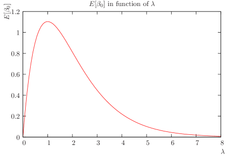
Figure 5. Variation of the mean number of clusters in function of $\lambda$ when $L=4$ and $\epsilon=1$.

The variance can be obtained also by Eq. (11):

$$\mbox{Var}(\beta_{0}(L))=(L-\epsilon)\lambda e^{-\epsilon\lambda}{\mathbf{1}}_{\left\{{L>\epsilon}\right\}}+(L-2\epsilon)\lambda^{2}e^{-2\epsilon\lambda}{\mathbf{1}}_{\left\{{L>2\epsilon}\right\}}\\ -(L-\epsilon)^{2}\lambda^{2}e^{-2\epsilon\lambda}{\mathbf{1}}_{\left\{{L>\epsilon}\right\}},$$

and under the condition that $L>2\epsilon$:

$$\mbox{Var}(\beta_{0}(L))=(L-\epsilon)\lambda e^{-\epsilon\lambda}+\epsilon(3\epsilon-2L)\lambda^{2}e^{-2\epsilon\lambda}.$$

Fig. 6

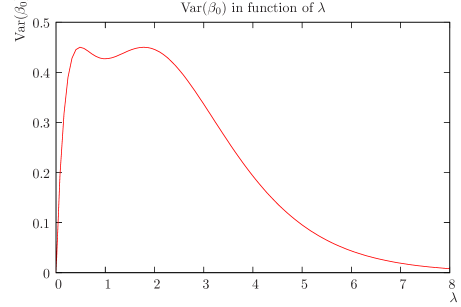
Figure 6. Behavior of the variance of the number of clusters in function of $\lambda$ when $L=4$ and $\epsilon=1$.

shows a plot of Var($\beta_{0}(L)$) in function of $\lambda$ for $L=4$ and $\epsilon=1$. We can expect that, when $\lambda$ is small compared to $\epsilon$, the plot should be approximatively linear, since there would not be too much connections in the network and the variance of the number of clusters should be close to the variance of the number of sensors given by $\lambda L$. Since $\beta_{0}(L)$ tends almost surely to 0 when $\lambda$ goes to infinity, Var$(\beta_{0}(L))$ should also tend to 0 in this case. Those two properties are observed in the plot. Besides, we find the critical points of this function, and again, $\lambda=1/\epsilon$ is one of them and at this value Var$(\beta_{0}(L))=(L/\epsilon)e^{-1}+(3-2L/\epsilon)e^{-1}$. The other two are the ones satisfying the transcendant equation:

$$\lambda e^{-\lambda\epsilon}=\frac{L-\epsilon}{2\epsilon(2L-3\epsilon)}\cdotp$$

By using the second derivative, we realize that $1/\epsilon$ is actually a minimum. Besides, if $L\leq 2\epsilon$, there is just one critical point, a maximum, at $\lambda=1/\epsilon$.

The last example in the section is performed with the result obtained in Theorem 9. We consider again $L=4$ and $\epsilon=1$ to obtain the following distributions:

$$\Pr(\beta_{0}(L)=0) = 1-3\lambda e^{-\lambda}+2\lambda^{2}e^{-2\lambda}-1/6\lambda^{3}e^{-3\lambda},$$

$$\Pr(\beta_{0}(L)=1) = 3\lambda e^{-\lambda}-4\lambda^{2}e^{-2\lambda}+1/2\lambda^{3}e^{-3\lambda},$$

$$\Pr(\beta_{0}(L)=2) = 2\lambda^{2}e^{-2\lambda}-1/2\lambda^{3}e^{-3\lambda},$$

$$\Pr(\beta_{0}(L)=3) = 1/6\lambda^{3}e^{-3\lambda},$$

$$\Pr(\beta_{0}(L)>3) = 0.$$

Those expressions are simple and they have at most four terms, since $L=4\epsilon$. We plot these functions in Fig. 7. The critical points on those plots at $\lambda=1/\epsilon$ are confirmed for the fact that, in function of $\lambda$, for every $n$, $\Pr(\chi(L)=n)$ can be represented as a sum

$$\sum_{i=0}^{j}q_{i,j}(\lambda e^{-\lambda\epsilon})^{i}$$

where the coefficients $q_{i,j}$ are constant in relation to $\lambda$. However, $(\lambda e^{-\lambda\epsilon})^{i}$ has a critical point at $\lambda=1/\epsilon$ for all $i>0$, so this should be also a critical point of $\Pr(\chi(L)=n)$. If $\lambda$ is small, we should expect that $\Pr(\chi(L)=0)$ is close to one, since it is likely to $N$ have no points. For this reason, in this region, $\Pr(\chi(L)=n)$ for $n>0$ is small. When $\lambda$ is large, we expect to have very large clusters, likely to be larger than $L$, so it is unlikely to have a complete cluster in the interval and, again, $\Pr(\chi(L)=0)$ approaches to the unity, while $\Pr(\chi(L)=n)$ for $n>0$ become again small.

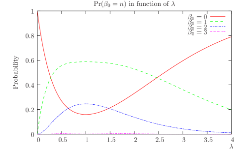
Figure 7. Probabilities of connectiveness, $\Pr(\beta_{0}(L)=n)$, for $n=0,1,2,3$, in function of $\lambda$ when $L=4$ and $\epsilon=1$.

References

[1]
J. Kahn, R. Katz, and K. Pister, “Mobile networking for smart dust,” in Intl. Conf. on Mobile Computing and Networking, (Seattle, WA), august 1999.
[2]
F. Lewis, Wireless Sensor Networks, ch. 2.
John Wiley, New York, 2004.
[3]
G. Pottie and W. Kaiser, “Wireless integrated network sensors,” Communications of the ACM, vol. 43, pp. 51–58, may 2000.
[4]
C.-Y. Chong and S. P. Kumar, “Sensor networks: Evolution, opportunities, and
challenges,” in Proceedings of IEEE, vol. 91, pp. 1247–1256, august
2003.
[5]
R. Ghrist, “Coverage and hole-detection in sensor networks via homology,” in
Fouth International Conference on Information Processing in Sensor
Networks (IPSN’05), UCLA, pp. 254–260, 2005.
[6]
V. de Silva and R. Ghrist, “Coordinate-free coverage in sensor networks with
controlled boundaries via homology,” International Journal of Robotics
Research, vol. 25, december 2006.
[7]
A. F. Siegel and L. Holst, “Covering the circle with random arcs of random
sizes,” Journal of Applied Probability, vol. 19, pp. 373–381, June
1982.
[8]
L. Holst, “On multiple covering of a circle with random arcs,” J. Appl.
Probab., vol. 17, no. 1, pp. 284–290, 1980.
[9]
P. Kumar, “New technological vistas for systems and control: the example of
wireless networks,” IEEE Control Systems Magazine, pp. 24–37, feb
2001.
[10]
M. Noori, S. Movaghati, and M. Ardakani, “Characterizing the path coverage of
random wireless sensor networks,” EURASIP Journal on Wireless and
Networking, 2010.
[11]
P. Manohar, S. S. Ram, and D. Manjunath, “Path coverage by a sensor field: the
nonhomogeneous case,” ACM Transactions on Sensor Networks, vol. 5,
March 2009.
[12]
R. Ghrist and A. Muhammad, “Coverage and hole-detection in sensor networks via
homology,” Information Processing in Sensor Networks, 2005. IPSN 2005.
Fourth International Symposium on, pp. 254–260, 2005.
[13]
R. L. Graham, D. E. Knuth, and O. Patashnik, Concrete Mathematics: A
Foudation for Computer Science, ch. 6.1, pp. 257–267.
Reading, MA: Addison-Wesley, 1994.
[14]
D. C. Wood, “Technical report 15-92,” tech. rep., University of Kent
computing Laboratory, University of Kent, Canterburry, 1992.
[15]
S. Roman, The Umbral of Calculus.
New York: Academic Press, 1984.