ac-dc voltage profile and four point impedance of a quantum driven system

Abstract

We investigate the behavior of the time-dependent voltage drop in a periodically driven quantum conductor sensed by weakly coupled dynamical voltages probes. We introduce the concepts of ac-dc local voltage and four point impedance in an electronic system driven by ac fields. We discuss the properties of the different components of these quantities in a simple model of a quantum pump, where two ac voltages oscillating with a phase lag are applied at the walls of a quantum dot.

I Introduction

In stationary transport through mesoscopic systems, the four-point terminal resistance is regarded as the proper concept to characterize the resistive behavior of the sample, free from the effects of the contact resistances. This concept has been introduced in Refs. L70, ; engq, , and further elaborated in Refs. BU8688, ; been, . Its behavior in different systems under dc-driving has been analyzed in several theoretical works. gram Recent experiments on semiconducting devices pic and carbon nanotubes gao ; makarovski constitute evidences that this quantity can be positive as well as negative at low temperatures, in agreement with theoretical predictions on the basis of coherent electronic transport. L70 ; engq ; BU8688 ; been ; gram

Time dependent quantum transport in ac driven small-size systems is receiving nowadays considerable theoretical and experimental attention. A variety of devices like quantum dots, electronic systems in the quantum Hall regime, quantum capacitors and graphene nanoribbons have been recently investigated experimentally. SMCG99 ; Chepe ; pumpex Among other interesting effects, the mechanisms for the induction of dc electronic and spin currents tdep1_spin_charge ; mobum ; brou0 ; brou ; mobup ; lilimos ; lilip ; lilisim ; otros , the behavior of the dc and t-resolved noise tdep2_noise1 ; tdep2_noise , the energy transport and the heat generation tdep3_heat have been analyzed.

While the experimental setups in some of these devices involve four-terminal measurements SMCG99 ; Chepe , the theoretical discussion on how to extend the definition of the four-point resistance in the context of time-dependent transport, has been considered only recently. In Ref. us, we have introduced the concept of a non-invasive dc voltage probe in a simple model of a quantum pump. We have extended the ideas of Refs. L70, ; engq, ; BU8688, ; been, ; gram, by representing the probe as a particle reservoir which is weakly coupled to the driven system at the point where the voltage is to be sensed. Then, the local dc voltage is defined as the value of the dc bias that has to be applied at the probe in order to satisfy the condition of a vanishing dc particle current between it and the driven system. A similar route has been recently followed to define the local temperature from the constraint of a vanishing dc heat current between the driven system and the probe, as a condition of local thermal equilibrium. temp The dc four point resistance is defined as the ratio between the dc voltage drop measured between two independent weakly coupled voltages probes and the dc pumped current circulating through the device. us In this “gedanken” setup, the two probes correspond to sensing the voltage difference between two points of the circuit by means of a dc voltimeter.

In the presence of ac fields, it is however interesting to characterize not only the dc but also the ac component of the voltage drop. The aim of this work is precisely to discuss the way to generalize the properties of a voltage probe in order to sense both the dc and the ac features in the voltage profile. Following this route, we are lead to the concept of four terminal impedance for a quantum driven system, as a concomitant extension of the concept of four terminal resistance. For sake of simplicity, we mainly focus on the weak driving regime. This corresponds to the so called adiabatic regime, where the period of the ac voltages is much larger than the typical time that an electron spends inside the structure (the dwell time), while the amplitudes of the potentials are much smaller than the energy scale characterizing the dynamics of the electrons within the structure. We also analyze these ideas in a simple model of a quantum pump device.

In Refs. brou, ; mobup, it has been pointed out that different contributions to the dc currents can be identified in setups under the action of both localized time-dependent potentials acting on the central structure and ac voltages at the reservoirs. The two most relevant contributions are (i) the one due to pure pumping processes, and (ii) the one due to the existence of a bias applied at the reservoirs. The latter part, in turn, may contain a component due to a dc bias and a component due to the rectification of the ac potentials. Besides these, there is an additional component in the dc current, which is due to the interference between the pumping and rectification processes. mobup ; lilimos In this work, we show that these different mechanisms affect the determination of the local voltage. One remarkable consequence of this fact is that the solely introduction of an ac voltage at the probe in order to detect time-dependent features at the structure, originates additional scattering processes that modify the dc voltage profile, even when the probe is weakly coupled to the sample.

The paper is organized as follows: In Sec. II the model for the driven structure and for the ac-dc voltage probe is introduced. We present the theoretical treatment based in non-equilibrium Green functions, used to evaluate the relevant physical quantities like the time-dependent currents along the device. In Sec. III we present results for the parameters characterizing the ac voltage profile as well as the four terminal impedance in a model for a quantum pump. Finally Sec. IV is devoted to the summary and conclusions.

II Theoretical treatment

II.1 Model

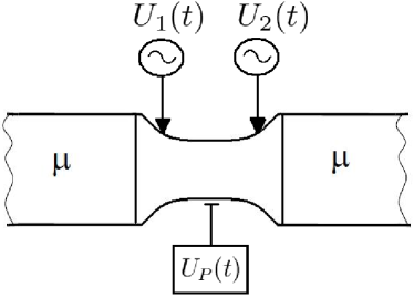
Figure 1: (Color on-line) Sketch of the setup to describe the ac-dc voltage profile. The central system is driven out-of equilibrium by external ac voltages $U_{1}(t)$ and $U_{2}(t)$, while it is in contact to left ($L$) and right ($R$) reservoirs at the same chemical potential $\mu$ and temperatures $T$. An additional reservoir (the probe) is weakly coupled to device under investigation. It has a bias with a dc component $\mu_{P}-\mu$ and an ac voltage $V_{P}\cos(\Omega_{0}t+\varphi_{P})$ that locally and instantaneously sets the equilibrium between the probe and the central system from the condition of a vanishing instantaneous current between both systems.

We consider the setup shown in the sketch of Fig.1, where a structure of a finite size driven by ac potentials is in contact to two reservoirs at the same temperature and chemical potential. For simplicity, we adopt units where $e=\hbar=1$. We describe the system by the following Hamiltonian:

$$H_{sys}(t) = H_{cen}(t)+\sum_{\alpha=L,R}(H_{\alpha}+H_{c,\alpha}),$$ (1)

where $L,R$ labels, respectively, left and right reservoirs. We assume a lattice model with $N$ sites for the central driven system:

$$H_{cen}(t) = H_{0}+H_{ac}(t),$$

$$H_{0} = -w\sum_{\langle ll^{\prime}\rangle}[c^{\dagger}_{l}c_{l^{\prime}}+H.c.]+\sum_{l}^{N}\varepsilon_{l}c^{\dagger}_{l}c_{l^{\prime}},$$

$$H_{ac}(t) = \sum_{l,l^{\prime}}[U_{l,l^{\prime}}(t)c^{\dagger}_{l}c_{l^{\prime}}+H.c.],$$ (2)

where $\langle ll^{\prime}\rangle$ denotes a pair of nearest-neighbor sites, and $w$ is a hopping parameter, while $U_{l,l^{\prime}}(t)=U^{0}_{l,l^{\prime}}\cos(\Omega_{0}t+\varphi_{l,l^{\prime}})$. Fig. 1 corresponds to an example where this ac potential has two local components. Assuming that the points of the structure at which the potentials act are labeled, respectively, by $l_{1}$ and $l_{2}$, the driving potential in this example reads: $U_{l,l^{\prime}}(t)=\delta_{l,l^{\prime}}[\delta_{l,l_{1}}U^{0}_{1}\cos(\Omega_{0}t+\varphi_{1})+\delta_{l,l_{2}}U^{0}_{2}\cos(\Omega_{0}t+\varphi_{2})]$.

The Hamiltonians for the $L$ and $R$ reservoirs correspond to free electrons:

$$H_{\alpha} = \sum_{k_{\alpha}}\varepsilon_{k_{\alpha}}c^{\dagger}_{k_{\alpha}}c_{k_{\alpha}},$$ (3)

having chemical potential $\mu$ and equal temperature. The contacts between the driven system and the reservoirs are described by tunneling Hamiltonians of the form:

$$H_{c,\alpha} = w_{\alpha}\sum_{k_{\alpha}}(c^{\dagger}_{k_{\alpha}}c_{l_{\alpha}}+H.c.),$$ (4)

where $l_{\alpha}$ labels the sites of the central lattice that are in contact with the reservoirs.

We now introduce the model for the ac-dc voltage probe. It consists in an additional reservoir of non-interacting electrons with a time-dependent bias voltage, which is weakly coupled to the central device at the point where the potential is to be sensed. The corresponding Hamiltonian for this system reads: mobup ; lilip ; jau

$$H_{P} = \sum_{p}[\varepsilon_{p}-U_{P}(t)]c^{\dagger}_{p}c_{p},$$ (5)

where $\varepsilon_{p}$ is the dispersion relation corresponding to the free electrons while the bias $U_{P}(t)$ is assumed to depend harmonically in time:

$$U_{P}(t)=\sum_{k=-\infty}^{+\infty}e^{-ik\Omega_{0}t}U_{P}^{(k)},$$ (6)

having a dc component $U_{P}^{(0)}=\mu_{P}-\mu$ and an ac component $U_{P}^{(ac)}=\sum_{k\neq 0}e^{-ik\Omega_{0}t}U_{P}^{(k)}$. The probe couples to the central device at the site $l_{P}$ through a tunneling term of the form:

$$H_{c,P} = w_{P}\sum_{p}(c^{\dagger}_{p}c_{l_{P}}+H.c.).$$ (7)

We assume that the probe is non-invasive, which implies that the tunneling parameter $w_{P}$ is so small that it does not affect the coherent nature of the transport processes along the driven central system. The key feature of the probe is that the potential $U_{P}(t)$ is adjusted in order to satisfy at every time the condition of a vanishing charge current $J_{P}(t)=0$ through its contact to the central device (see Fig. 1). In this way, the potential $U_{P}(t)$ is the one satisfying at every time local equilibrium regarding charge flow between the central system and the probe. For this reason, it is interpreted as the time-dependent local potential of the system sensed by the probe. This definition is precisely an extension of the one originally proposed by Engquist and Anderson engq to the case of a system driven by time-dependent fields. It also generalizes the definition of the dc voltage probe that we have introduced in Ref. us, , where we have followed a procedure equivalent to the present one but with $U_{P}^{(ac)}=0$. As we shall see, to include an ac component in the probe voltage introduces significant corrections to the sensed dc voltage.

II.2 Sensing an ac-dc local voltage with a probe

The model for the probe we have introduced in the previous subsection is completely general. For sake of simplicity, in what follows we focus on weak driving. Therefore, we assume that the driving potentials $U(t)$ depend at least on two parameters, in order to produce adiabatic dc currents at low driving frequencies $\Omega_{0}$. brou ; mobup ; lilip We also assume that the corresponding driving amplitudes are small enough to generate time-dependent currents composed of a single harmonic besides the dc component. In particular, we assume that the time-dependent current flowing into the reservoir $\alpha$ has the form:

$$J_{\alpha}(t) = \sum_{k=-1}^{1}J^{(k)}_{\alpha}e^{-ik\Omega_{0}t},$$ (8)

which motivates assuming the following functional form for the ac voltage at the probe:

$$U_{P}(t) = \mu_{P}-\mu+V_{P}\cos(\Omega_{0}t+\varphi_{P}).$$ (9)

This means that the local voltage sensed by the probe becomes characterized by the dc bias $\mu_{P}-\mu$, as well as the amplitude $V_{P}$ and the phase $\varphi_{P}$ of the ac component. These three parameters are adjusted to satisfy the following set of three equations:

$$J^{(k)}_{P}=0,\;\;\;\;k=-1,0,1,$$ (10)

with $J^{(1)}_{P}=[J^{(-1)}_{P}]^{*}$.

The evaluation of the different harmonics of the ac current can be done by resorting to non-equilibrium Green function formalism. Following Ref. lilip, , we express the time-dependent current flowing through the contact between the central system and the probe in terms of Green functions:

$$J_{P}(t) = \int_{-\infty}^{+\infty}dt_{1}\{G^{R}_{l_{P},l_{P}}(t,t_{1})\Sigma^{<}_{P}(t_{1},t)$$ (11)

$$+G^{<}_{l_{P},l_{P}}(t,t_{1})\Sigma^{A}_{P}(t_{1},t)\},$$

with:

$$\Sigma^{A}_{P}(t,t^{\prime}) = i\Theta(t^{\prime}-t)\phi(t,t^{\prime})\int\frac{d\omega}{2\pi}e^{-i\omega(t-t^{\prime})}\Gamma_{P}(\omega),$$

$$\Sigma^{<}_{P}(t,t^{\prime}) = i\phi(t,t^{\prime})\int\frac{d\omega}{2\pi}e^{-i\omega(t-t^{\prime})}f(\omega)\Gamma_{P}(\omega),$$ (12)

with

$$\phi(t,t^{\prime}) = e^{-i\int^{t}_{t^{\prime}}dt_{1}U_{P}(t_{1})},$$ (13)

being $\Gamma_{P}(\omega)=2\pi|w_{P}|^{2}\sum_{p}\delta(\omega-\varepsilon_{p})$, the spectral density associated to the self-energy due to the escape of the electrons from the central device to the probe. We consider a wide-band model for this system, which implies a constant density of states $\Gamma_{P}(\omega)\sim\Gamma,\;\forall\omega$. The Fermi function $f(\omega)=1/(e^{\beta(\omega-\mu)}+1)$, depends on the chemical potential $\mu$ of the $L$ and $R$ reservoirs, which we take as a reference and on the temperature $1/\beta$ that we assume to be same for all the reservoirs. The retarded and lesser Green functions are, respectively, evaluated by solving Dyson equations:

$$-i\partial_{t^{\prime}}\hat{G}^{R}(t,t^{\prime})-\hat{G}^{R}(t,t^{\prime})\hat{H}_{sys}(t)$$

$$-\int dt_{1}\hat{G}^{R}(t,t_{1})\hat{\Sigma}^{R}(t_{1},t^{\prime})=\hat{1}\delta(t-t^{\prime}),$$ (14)

$$\!\!\!\hat{G}^{<}(t,t^{\prime})=\int dt_{1}dt_{2}\hat{G}^{R}(t,t_{1})\hat{\Sigma}^{<}(t_{1},t_{2})\hat{G}^{A}(t_{1},t^{\prime}),$$

with $\hat{G}^{A}(t,t^{\prime})=[\hat{G}^{R}(t^{\prime},t)]^{\dagger}$ and $\hat{\Sigma}^{A}(t,t^{\prime})=[\hat{\Sigma}^{R}(t^{\prime},t)]^{\dagger}$. The elements of the Green function matrices are defined over the sites of the central device and $\hat{1}$ denotes the identity matrix in this space. Similarly, the Hamiltonian matrix $\hat{H}_{sys}(t)$ contains the matrix elements of the Hamiltonian (1), while the self-energy matrix contains non-vanishing elements only at the sites $l_{\alpha}$, that are in contact to the reservoirs $\alpha=L,R,P$.

As in previous works lilip ; lilimos ; us , we introduce the following representation for the retarded Green function:

$$\hat{G}^{R}(t,t^{\prime}) = \sum_{k}\int\frac{d\omega}{2\pi}e^{-ik\Omega_{0}t}e^{-i\omega(t-t^{\prime})}\hat{\cal G}(k,\omega).$$ (15)

In addition, for weak driving voltages, it is natural to assume also weak amplitudes for the dc and ac voltages of the probe. Thus, the exponential of Eq. (16) simplifies to:

$$\phi(t,t^{\prime}) \sim \{1-i[(\mu_{P}-\mu)(t-t^{\prime})$$ (16)

$$+\int^{t}_{t^{\prime}}dt_{1}V_{P}\cos(\Omega_{0}t_{1}+\varphi_{P})]\}.$$

Introducing expressions Eqs.(15) and (16) in Eq.(11), taking into account the assumption of a low driving frequency by keeping terms up to ${\cal O}(\Omega_{0})$, and keeping terms up to ${\cal O}(w_{P})$ due to the non-invasiveness of the probe, we arrive, after some algebra, to the following expression for current flowing through the contact between the central system and the probe:

$$J_{P}(t) = \sum_{k=-1}^{1}\sum_{\alpha=L,R,k^{\prime}}e^{-ik\Omega_{0}t}\int\frac{d\omega}{2\pi}\frac{\partial f(\omega)}{\partial\omega}\Gamma_{\alpha}(\omega)\Gamma_{P}(\omega)$$ (17)

$$\times{\cal G}_{l_{P},l_{\alpha}}(k+k^{\prime},\omega)[{\cal G}_{l_{P},l_{\alpha}}(k^{\prime},\omega)]^{*}\times$$

$$[V_{P}\cos(\Omega_{0}t+\varphi_{P})-\mu+\mu_{P}-k^{\prime}\Omega_{0}]-i\sum_{k=-1}^{1}k\Omega_{0}$$

$$\times e^{ik\Omega_{0}t}\int\frac{d\omega}{2\pi}\frac{\partial f(\omega)}{\partial\omega}[{\cal G}_{l_{P},l_{P}}(k,\omega)]^{*}\Gamma_{P}(\omega).$$

As discussed in Refs. mobup, ; lilimos, , it is possible to split the time-dependent current into different components:

$$J_{P}(t)=J^{pump}(t)+J^{bias}(t).$$ (18)

The first one corresponds to pure pumping processes and behaves like $J^{pump}(t)\propto\Omega_{0}$, while the other one is the contribution due to the existence of a bias, and behaves like $J^{bias}(t)\propto U_{P}(t)$. In this approximation we are neglecting the interference term, which is $\propto\Omega_{0}U_{P}(t)$. In terms of the driving parameters, the latter term contributes at ${\cal O}(\Omega_{0}U_{0}^{4})$ to the dc component and at ${\cal O}(\Omega_{0}U_{0}^{3})$ to the first harmonic of the probe voltage.

For weak driving, the Dyson equation Eq. II.2 can be solved perturbatively. lilip The terms necessary to evaluate the conditions of Eq. (10) exactly up to ${\cal O}(U_{0}^{2})$, ${\cal O}(\Omega_{0})$ and ${\cal O}(w_{P})$ are:

$$\hat{G}(t,\omega)\sim\sum_{k=-1}^{1}\hat{\cal G}(k,\omega)e^{-ik\Omega_{0}t},$$ (19)

with

$$\hat{\cal G}(0,\omega) \sim \hat{G}^{0}(\omega),$$

$$\hat{\cal G}(\pm 1,\omega) \sim \hat{G}^{0}(\omega)\hat{V}^{(\pm 1)}\hat{G}^{0}(\omega),$$ (20)

where $\hat{G}^{0}(\omega)$ is the equilibrium retarded Green function of the central system described by the Hamiltonian $H_{0}$, coupled only to the $L$ and $R$ reservoirs, while:

$$V^{(\pm 1)}_{l,l^{\prime}}=\frac{U^{0}_{l,l^{\prime}}}{2}e^{\mp i\varphi_{l,l^{\prime}}}.$$ (21)

Inserting these functions into in the time-dependent current Eq. (17) and imposing the conditions Eq. (10), we obtain the following set of linear coupled equations that must be fulfilled in order to have a vanishing time-dependent current:

$$\mu-\mu_{P} = \Omega_{0}\lambda^{(0)}_{P}+\mbox{Re}\{V_{P}e^{i\varphi_{P}}\lambda^{(1)}_{P}\},$$ (22)

$$\frac{V_{P}}{2}e^{-i\varphi_{P}} = \Omega_{0}\lambda^{(2)}_{P}+(\mu-\mu_{P})\lambda^{(1)}_{P},$$ (23)

being

$$\lambda^{(0)}_{P} = -\frac{\sum_{\alpha}\sum_{k=\pm 1}k|{\cal G}_{l_{P},l_{\alpha}}(k,\mu)|^{2}\Gamma_{\alpha}(\mu)}{\Lambda_{P}},$$

$$\lambda^{(1)}_{P} = \frac{\sum_{\alpha}\sum_{k=-1}^{0}{\cal G}_{l_{P},l_{\alpha}}(k+1,\mu)[{\cal G}_{l_{P},l_{\alpha}}(k,\mu)]^{*}\Gamma_{\alpha}(\mu)}{\Lambda_{P}},$$

$$\lambda^{(2)}_{P} = -\frac{\sum_{\alpha}{\cal G}_{l_{P},l_{\alpha}}(0,\mu)[{\cal G}_{l_{P},l_{\alpha}}(-1,\mu)]^{*}\Gamma_{\alpha}(\mu)}{\Lambda_{P}}$$

$$-i\frac{[{\cal G}_{l_{P},l_{P}}(-1,\mu)]^{*}}{\Lambda_{P}},$$

$$\Lambda_{P} = \sum_{\alpha}|G^{0}_{l_{P},l_{\alpha}}(\mu)|^{2}\Gamma_{\alpha}(\mu),$$ (24)

where the sum in $\alpha$ runs over $L,R$ and, for simplicity, we have assumed zero temperature. It is interesting to notice in the above equations, that the very existence of an ac component in the voltage probe ($V_{P}$) modifies the dc component of the voltage profile $\mu_{P}-\mu$.

Finally, keeping only terms up to ${\cal O}(U_{0}^{2})$ in the solution of Eqs. (22,23), we obtain the dc and ac components of the voltage profile sensed by the voltage probe. They respectively read:

$$\mu-\mu_{P} = \Omega_{0}\{\lambda^{(0)}_{P}+\frac{1}{2}\mbox{Re}[\lambda^{(1)}_{P}(\lambda^{(2)}_{P})^{*}]\},$$ (25)

$$V_{P}e^{-i\varphi_{P}} = 2\Omega_{0}\lambda^{(2)}_{P},$$ (26)

where dc the component is $\propto\Omega_{0}U_{0}^{2}$, while the ac one is $\propto\Omega_{0}U_{0}$.

At this point it is important to compare Eq. (25) with the result obtained for the case of a dc probe, as the one considered in Ref. us, . The latter case corresponds to take $V_{P}=0$, in the above expressions, which in turn leads to a dc voltage profile $\mu_{P}-\mu$ given only by the first term of Eq. (25). It is easy to verify that this result coincides with Eq. (16) of our previous work. us ; note The dc voltage probe senses scattering events at static barriers, like walls and impurities of the structure, as well as at the dynamical pumping centers, with the characteristic that they take place within the same Floquet channel. These processes are contained in the first term ($\lambda^{(0)}_{P}$) of the above expressions. On the other hand, the ac component of the voltage profile senses additional effects due to scattering processes between different Floquet components. These are collected into the terms $\lambda^{(1)}_{P}$ and $\lambda^{(2)}_{P}$ of Eq.(25). The remarkable and new feature that the ac-dc voltage probe brings about is contained in these inter-Floquet scattering processes that lead to a correction of the same order in the driven parameters, i.e. an extra term $\propto\Omega_{0}U_{0}^{2}$, that has to be added to the result obtained with a dc voltage probe.

II.3 Four terminal impedance

The dc component of the current entering the $L$ and $R$ reservoirs satisfies the relation $J_{L}^{(0)}=-J_{R}^{(0)}$. However, the higher harmonics $J_{\alpha}^{(\pm 1)}$ are not expected to satisfy such a condition (see Ref. tdep2_noise1, ). This is because there may be instantaneous accumulation of charge with vanishing average along the structure. Therefore, in order to define the impedance of the device, we choose the current flowing through the left contact as a reference.

For weak driving, the time-dependent currents (8) flowing into the $L$ and $R$ contacts have the following components:

$$J_{\alpha}^{(0)} = \Omega_{0}\sum_{\beta=L,R}\sum_{k}\Gamma_{\alpha}(\mu)\Gamma_{\beta}(\mu)$$

$$\times k|{\cal G}_{l_{\alpha},l_{\beta}}(k,\mu)|^{2},$$

$$J_{\alpha}^{(\pm 1)} = \Omega_{0}\sum_{\beta=L,R}\sum_{k=\mp 1,0}\Gamma_{\alpha}(\mu)\Gamma_{\beta}(\mu)$$ (27)

$$\times k{\cal G}_{l_{\alpha},l_{\beta}}(k\pm 1,\mu){\cal G}_{l_{\alpha},l_{\beta}}(k,\mu)^{*}$$

$$\mp i{\cal G}_{l_{\alpha},l_{\alpha}}(\mp 1,\mu)^{*}\Gamma_{\alpha}(\mu)\},$$

being $J_{\alpha}^{(1)}=[J_{\alpha}^{(-1)}]^{*}$, with the Green functions given by (19) and (II.2).

In a four terminal measurement, with ac-dc non-invasive probes, the voltage drop between the points $l_{P}$ and $l_{P^{\prime}}$ is simply the difference of the voltage sensed by each probe, regarding each of them as independent of one another, thus:

$$\Delta V(t)=\sum_{k=-1}^{1}\Delta V^{(k)}e^{-ik\Omega_{0}t},$$ (28)

being the ac and dc components, respectively:

$$\Delta V^{(\pm 1)} = V_{P}e^{\pm i\varphi_{P}}-V_{P^{\prime}}e^{\pm i\varphi_{P^{\prime}}},$$

$$\Delta V^{(0)} = \mu_{P}-\mu_{P^{\prime}}.$$ (29)

Thus, the four-point impedance also has ac and dc components defined as follows:

$$Z^{(k)}=\frac{\Delta V^{(k)}}{J_{L}^{(k)}},k=-1,0,1,$$ (30)

being $Z^{(1)}=[Z^{(-1)}]^{*}$. In linear circuits with ac and dc sources, the dc component of the impedance, $Z^{(0)}$ is simply the resistance, and it coincides with the real part of $Z^{(1)}$. In our quantum case, we cannot provide any proof on the validity of such a relation between the two components of the impedance, and we must simply regard them as providing different pieces of information about the driven system.

Of particular interest is the behavior of $Z^{(0)}$, which should be regarded as an extended definition of the dc four-point resistance $R_{4t}$ we have introduced in Ref. us, . In the next section we present results for a particular model of driven system. In general, we can notice that the four-terminal resistance sensed by dc probes is associated with the first term of Eq. (25):

$$R_{4t}=\Omega_{0}\frac{\lambda^{(0)}_{P^{\prime}}-\lambda^{(0)}_{P}}{J_{L}^{(0)}}.$$ (31)

The dc impedance contains an additional term, which is of the same order of magnitude, associated to scattering processes mediated by the ac voltage of the probe:

$$Z^{(0)}=R_{4t}+\Omega_{0}\frac{\mbox{Re}[\lambda^{(1)}_{P^{\prime}}(\lambda^{(2)}_{P^{\prime}})^{*}-\lambda^{(1)}_{P}(\lambda^{(2)}_{P})^{*}]}{2J_{L}^{(0)}}.$$ (32)

III Results for a simple model of a quantum pump

We now examine the concepts introduced in the previous section in the context of a quantum pump device. We consider a simple model where two ac gate potentials with the same amplitude $V_{0}$ oscillate with a phase-lag $\delta$ at two barriers confining a quantum dot. The dot and barriers are described by the Hamiltonian $H_{0}$ introduced in section II.1, with hopping between nearest neighbor positions on a one-dimensional lattice of $N$ sites, and barriers at the positions $l_{A}$ and $l_{B}$ of that lattice:

$$\varepsilon_{l,l^{\prime}}=\delta_{l,l^{\prime}}[\delta_{l,l_{A}}+\delta_{l,l_{B}}]E_{B}.$$ (33)

The driving terms read:

$$U_{l,l^{\prime}}=V_{0}\delta_{l,l^{\prime}}[\cos(\Omega_{0}t+\delta)\delta_{l,l_{A}}+\cos(\Omega_{0}t)\delta_{l,l_{B}}].$$ (34)

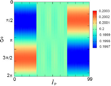
Figure 2: (Color on-line) Contour plot for the local dc component of the voltage $\mu_{P}$ sensed by the ac-dc voltage probe as function of the probe position $l_{P}$ along the system (horizontal axis) and the phase lag $\delta$. We consider a a quantum pump modeled by a driven chain with by $N=99$ sites with two barriers of height $E_{B}=0.2$ located at $l_{A}=30$ and $l_{B}=70$ as indicated by the vertical dashed lines. The chemical potential is $\mu=0.2$, which corresponds to $k_{F}=1.47$.

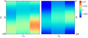
Figure 3: (Color on-line) Contour plot for the real (left panel) and imaginary part (right panel) of the ac component of the local potential $V_{P}e^{i\varphi_{P}}$ sensed by the ac-dc voltage probe as function of the probe position $l_{P}$ along the system (horizontal axis) and the phase lag $\delta$. Other parameters are the same as in Fig. 2.

The behavior of the dc and ac components of the voltage profile are shown, respectively, in Figs. 2 and 3, as functions of the position of the structure at which the probe is connected, $l_{P}$, and the phase-lag $\delta$ of the pumping potentials. In the case case of the ac component, we plot separately the behavior of the real and imaginary part of $V_{P}e^{i\varphi_{P}}$.

As discussed in section II.2, the ac-dc voltage probe senses a profile which significantly differs from the one sensed by a pure dc probe like the one we have considered in Ref. us, . This is because, the dc probe measures just the scattering processes that take place within a single Floquet channel, which are described by only the first term of Eq. (25). Instead, the additional ac components of voltage of the probe, $V_{P}^{\pm i\varphi_{P}}$, mediate scattering processes between different Floquet channels. The consequence is that the dc component of the profile sensed by the ac-dc probe contains, in addition, the second term of Eq. (25), which is of the same order of magnitude as the first one.

In order to make clear the difference between the two procedures of defining the dc component of the voltage profile, we plot the prediction of Eq. (25) for a set of representative values of the phase-lag $\delta$ in Fig. 4, also showing in dashed lines the prediction obtained from a pure dc probe like the one of Ref. us, . We notice that several interesting features can be identified in the voltage landscape for the case of the general ac-dc probe.

A first point worth of mention is that for the present system, which contains two pumping potentials with the same amplitude, the dc voltage profile sensed by a dc probe is flat along the structure and equal to zero when $\delta=0,\pi$. This behavior goes in line with the behavior of the dc-current along the structure, which vanishes for these values of the phase-lag as a consequence of the symmetries of the system. lilisim Moreover, it can be shown that for weak driving the dc current in this model behaves like $J^{0}\propto\Omega_{0}(V_{0})^{2}\sin(\delta)$, brou0 ; lilip and that for a fixed position of the probe, the dc voltage sensed by the dc probe follows exactly this behavior as a function of $\delta$. us In the case of the probe containing the additional ac voltage, the dc and ac components of the current along the structure are not affected by the probe, provided that it is weakly coupled. However, the additional inter-Floquet scattering processes mediated by the probe contribute to break symmetries and the dc profile is no longer an odd function of $\delta$, displaying non-vanishing features for $\delta=0,\pi$, as shown in Figs. 2 and 4. Our results show that the dc profile remains invariant under the following simultaneous transformations: $\delta\rightarrow-\delta;\;\;x\rightarrow-x$, where the latter operation denotes a spatial inversion with respect to the center of the structure (see Fig. 2). On the other hand, the analysis of the ac component of the voltage shown in Fig. 3 cast the invariance of the amplitude $V_{P}$ under the simultaneous transformation: $\delta\rightarrow-\delta;\;\;x\rightarrow-x;\;\;\varphi_{P}\rightarrow\varphi_{P}+\delta$. These symmetry properties are rather expected and fully consistent with the symmetry properties of the structure we are studying. However, we stress the remarkable fact that the dc voltage profile does not follow as a function of $\delta$ the behavior of the dc component of the current, as it is the case of the one defined from the pure dc probe. In the simple one-channel model we are considering, we cannot analyze the symmetry properties of the voltage profile in the presence of a magnetic field. In general, in the presence of a magnetic flux $B$, the non-interacting Green function satisfies the following symmetry: $\hat{G}^{0}(B,\omega)\rightarrow[\hat{G}^{0}(-B,\omega)]^{t}$, where the superscript $t$ denotes the transposed matrix. The way in which this transformation affects the voltages (22) and (23) is not obvious and is expected to be model-dependent. This is also the case of the dc pumped current, as discussed in previous works. mobum ; brou0

Another feature worth of notice is the pattern distinguished as a sequence of fringes in Figs. 2 and 3 and as oscillations of the dc and ac voltage landscapes of Figs. 4 and 5. The ultimate origin of these features is the existence of Friedel oscillations. For this reason, they show the characteristic spatial period of $2k_{F}$. In fact, it can be verified that the function $A\sin(2k_{F}l_{P}+\alpha)$, with suitable factors $A$ and $\alpha$, and $l_{P}$ adopting integer values (recall that we are studying a lattice model), displays the same plot as the oscillatory part of the plots shown in this figure, for the considered value of $k_{F}$. The sources for these oscillations are the different scattering centers of static and dynamical character. In particular, each of the two barriers of the structure, defined in the static profile (33), behaves like a static impurity which generates usual Friedel oscillations.gram On top of this, we also have dynamical scattering centers due to the pumping potentials. The consequence is the generation of $2k_{F}$ oscillations in both dc and ac components of the local density of states along the system.us The ensuing scattering processes being encoded within the different components of the Green function $G(k,\omega),k=-1,0,1$ and are detected in the dc as well as in the ac components of the voltage probe. The oscillations generated at the different sources, interfere and may become vanishingly small within some regions of the sample, depending on the value of the phase-lag $\delta$ (see, for example the central region between the two barriers in the two left-hand panels of Fig. 4 and in the top panels of Fig. 6). Notice that, besides the oscillations, the ac-voltage at the probe leads to a dc voltage drop that can be as large as twice the magnitude defined by a pure dc probe. This feature is important since in real experiments like that of Ref. SMCG99, , it is the voltage drop the measured quantity from where the pumped dc current is inferred. The dc voltage drop sensed by a pure dc probe is related to this current by a simple multiplicative factor, the dc four point resistance $R_{4t}$, which is expected to depend only on the properties of the sample. However, the presence of an ac voltage at probe can increase the dc voltage drop in a way that when simply dividing this quantity by $R_{4t}$, the inferred dc current can significantly differ from the actual one. In Refs. brou, ; mobup, it has been pointed out that the presence of voltage probes could increase the intensity of the dc current through the structure, by adding to the pumped current a contribution due to rectification mechanisms. Our results suggest that the dc current through the structure may remain unaffected by the probe, but when its magnitude is obtained by naively dividing the dc voltage drop by some estimate for $R_{4t}$, we could conclude that it is much larger than its actual value.

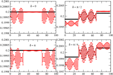
Figure 4: (Color on-line) The local dc component of the voltage $\mu_{P}$ sensed by the ac-dc voltage probe as function of the probe position $l_{P}$ along the system for different phase lags $\delta$, which are indicated in the Fig. In dashed lines, we indicate the profile corresponding to sensing with a dc probe. Other parameters are the same as in Fig. 2.

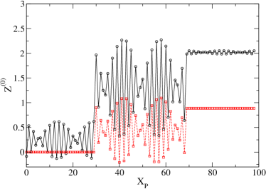
Figure 5: (Color on-line) The real (left) and imaginary (right) local ac component of the voltage $V_{P}e^{i\varphi_{P}}$ sensed by the ac-dc voltage probe as function of the probe position $l_{P}$ along the system for different phase-lags $\delta=0,\pi/2,\pi$, (top to bottom). Other parameters are the same as in Fig. 2.

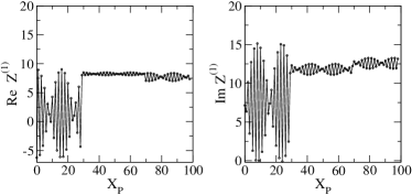
Figure 6: (Color on-line) The dc component of the impedance $Z^{(0)}$, connecting the first probe at $l_{P}=10$, as a function of the position of the second probe $l_{P^{\prime}}$ for $\delta=\pi/2$. The four terminal resistance $R_{4t}$ determined by a dc probe is also plotted in dashed lines. Other parameters are the same as in Fig. 2.

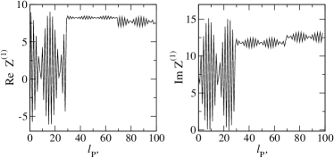
Figure 7: (Color on-line) Real (left panel) and imaginary (right panel) parts of the ac component of the impedance $Z^{(1)}$, connecting the first probe at $l_{P}=10$, as function of the position of the second probe $l_{P^{\prime}}$ for $\delta=\pi/2$, which are indicated in the Fig. Other parameters are the same as in Fig. 2.

Finally, we show in Figs. 6 and 7, respectively, the dc and ac components of the impedance for a particular value of the phase-lag. As discussed in section II.3, the dc component $Z^{(0)}$ differs from the dc four-terminal resistance $R_{4t}$ by the term due to scattering processes mediated by the ac potential of the probe. In Ref. us, we have shown for the present simple model of a quantum pump, that $R_{4t}$ of the full device, defined from a dc four terminal measurement with probes connected outside the driven region, is a universal property of the system, independent of the driving mechanism. Namely, it coincides with the one defined when the transport is induced by an equivalent dc voltage applied between the $L$ and $R$ reservoirs. On the contrary, the impedances $Z^{(0)}$ and $Z^{(1)}$, strongly depend on the positions where the probes are connected and account for the spacial oscillations of the voltage profile. Irrespectively of the position of the probes, for a given $\delta$, the behavior of the impedances along the structure contain the $2k_{F}$ oscillations of the voltage profiles.

IV Summary and conclusions

In this work we have introduced the theoretical concept of the ac-dc voltage probe, as a weakly coupled reservoir with a time-dependent voltage which instantaneously adapt to fulfill the local equilibrium condition of both dc and time-dependent current flowing between the driven system and the probe. We have focused on the weak driving regime, where the currents, as well as the probe voltage contain a single harmonic on top of their dc components. The procedure we have introduced, can be generalized to consider stronger driving and include additional harmonics. Under the assumption of non-invasive probes, the information of the voltage drop is enough to define the four-point impedance.

We have found that the dc component of the voltage defined in this way, differs from the one defined by a pure dc voltage probe. In particular, the ac-dc probe is able to capture scattering processes between different Floquet channels that are not detected by the pure dc one. These additional processes are of the same order of magnitude as the inter-Floquet ones and may introduce relevant qualitative features in the behavior of the voltage profile. In the particular case of a quantum pump with two ac potentials oscillating with a phase-lag, the dc voltage profile does not follow the same functional behavior with the phase-lag observed in the dc current. This feature also plagues the behavior of the dc component of the impedance $Z^{0}$. As a consequence, unlike the dc four point resistance $R_{4t}$, the dc impedance is not a universal quantity which depends on just the geometrical properties of the structure, but also depends on the position at which the voltage probes are connected.

One of the important messages of these theoretical ideas towards the experimental realm is related to the inference of the behavior of the dc current induced in the quantum pump from a four-terminal voltage measurement. The relation between these two quantities is not a simple factor as it could be naively expected. In Refs. brou, and mobup, it was discussed that the ac potentials of the voltage probes used in four terminal measurements in quantum pumps, as in the experiment by Switkes and coworkers SMCG99 , could act as additional sources and result in a dc current higher than the one induced by bare pumping potentials. In this work, we have considered non-invasive probes, which do not induce additional rectified currents through the structure. We have, however, shown that they anyway introduce additional scattering processes with the outcome of additional features in the sensed voltage landscape.

V Acknowledgements

We thank M. J. Sanchez for many discussions. We acknowledge support from CONICET, PIP 1212-09, UBACYT, Argentina, and J. S. Guggenheim Foundation (LA).

References

- (1) R. Landauer, Philos. Mag. 21, 863 (1970). R. Landauer, J. Phys. Cond. Matter, 1, 8099,(1989).
- (2) H. L. Engquist and P. W. Anderson, Phys. Rev. B 24, 1151, (1981).
- (3) M. Büttiker, Phys. Lett. 57, 1761 (1986). M. Büttiker, IBM J. Res. Dev, 32, 317 (1988); ibid 50, 2502 (1994).
- (4) C. W. J. Beenakker and H. van Houten, Phys. Rev. B 39, 10445 (1989).
- (5) V. A. Gopar, M. Martinez, and P. A. Mello, Phys. Rev. B 50, 2502 (1994); T. Gramespacher and M. Büttiker, Phys. Rev. B 56, 13026 (1997); L. Arrachea, C. Naón and M. Salvay, Phys. Rev. B 77, 233105 (2008). A. Terasawa, T. Tada and Satoshi Watanabe, Phys. Rev. B 79, 195436 (2009).
- (6) R. de Picciotto, H. L. Stormer, L. N. Pfeiffer, K. W. Baldwin and K. W. West, Nature 411, 51 (2001).
- (7) B. Gao, Y. F. Chen, M. S. Fuhrer, D. C. Glattli, and A. Bachtold, Phys. Rev. Lett. 95 196802 (2005).
- (8) A. Makarovski, A. Zhukov, J. Liu, and G. Finkelstein, Phys. Rev. B 76, 161405(R) (2007).
- (9) M. Switkes, C. M. Marcus, K. Campman, and A. C. Gossard, Science 283, 1905 (1999).
- (10) A. D. Chepelianskii and H. Bouchiat, Phys. Rev. Lett. 102, 086810 (2009).
- (11) L. J. Geerligs, V. F. Anderegg, P. A. M. Holweg, J. E. Mooij, H. Pothier, D. Esteve, C. Urbina, and M. H. Devoret, Phys. Rev. Lett. 64, 2691 (1990); L. Di Carlo, C. M. Marcus and J. S. Harris, Jr. , Phys. Rev. Lett. 91, 246804 (2003); M. D. Blumenthal, B. Kaestner, L. Li, S. Giblin, T. J. B. M. Hanssen, M. Pepper, D. Anderson, G. Jones, and D. A. Ritchie, Nature Physics 3, 343 (2007); J. Gabelli, G. Fève, J.-M. Berroir, B. Plaçais, A. Cavanna, B. Etienne, Y. Jin, and D. C. Glattli, Science 313, 499 (2006); G. Fè ve, A. Mahé, J.-M. Berroir, T. Kontos, B. Plaçais, D. C. Glattli, A. Cavanna, B. Etienne, and Y. Jin, Science 316, 1169 (2007).
- (12) P. Sharma and C. Chamon, Phys. Rev. Lett. 87, 096401 (2001); E. R. Mucciolo, C. Chamon, and C. M. Marcus, Phys. Rev. Lett. 89, 146802 (2002); M. Moskalets and M. Büttiker, Phys. Rev. B 66, 205320 (2002) and Phys. Rev. B 78, 035301 (2008); I.L. Aleiner and A.V. Andreev, Phys. Rev. Lett. 81, 1286 (1998); J. E. Avron, A. Elgart, G. M. Graf, and L. Sadun, Phys. Rev. Lett. 87, 236601 (2001); V. Kashcheyevs, A. Aharony, and O. Entin-Wohlman, Phys. Rev. B 69, 195301 (2004); J. Splettstoesser, M. Governale, J. König, and R. Fazio, Phys. Rev. Lett. 95, 246803 (2005); E. Faizabadi, Phys. Rev. B 76, 075307 (2007); S. E. Nigg, R. López, and M. Büttiker, Phys. Rev. Lett. 97, 206804 (2006); A. Agarwal and D. Sen, Phys. Rev. B 76, 035308 (2007); V. Moldoveanu, V. Gudmundsson, and A. Manolescu, Phys. Rev. B 76, 165308 (2007); R. Zhu, H. Chen, App. Phys. Lett. 95, 122111 (2009); A. R. Hernández, F. A. Pinheiro, C. H. Lewenkopf, and E. R. Mucciolo, Phys. Rev. B 80, 115311 (2009); F. Cavaliere, M. Governale, and J. König, Phys. Rev. Lett. 103 136801 (2009); N. Winkler, M. Governale, and J. König, Phys. Rev. B, 79, 235309 (2009).
- (13) F. Zhou, B. Spivak, and B. Altshuler, Phys. Rev. Lett. 82, 608 (1999); I. L. Aleiner, B. L. Altshuler and A. Kamenev, Phys. Rev. B 62, 10373 (2000); M. G. Vavilov, V. Ambegaokar and I. L. Aleiner, Phys. Rev. B 63, 195313 (2001); M. Moskalets and M. Büttiker, Phys. Rev. B 72, 035324 (2005).
- (14) P. W. Brouwer, Phys. Rev. B 58, R10135 (1998).
- (15) P. W. Brouwer, Phys. Rev. B 63, 121303 (2001); M.L. Polianski and P. W. Brouwer, Phys. Rev. B 64, 075304 (2001).
- (16) M. Moskalets and M. Büttiker, Phys. Rev. B 69, 205316 (2004).
- (17) L. Arrachea and M. Moskalets, Phys. Rev. B 74, 245322 (2006).
- (18) L. Arrachea, Phys. Rev. B 72, 125349 (2005); Phys. Rev. B, 75, 035319 (2007).
- (19) L. Arrachea, Phys. Rev. B 72, 121306 (2005).
- (20) G. Platero and R. Aguado, R. 2004, Phys. Rep. 395, 1 (2004); S. Kohler, J. Lehmann, and P. Hänggi, Phys. Rep. 406 (2005); L. Foa Torres and G. Cuniberti, App. Phys. Lett. 94 222103 (2009); K. Das and S. Aubin, Phys. Rev. Lett. 103, 123007 (2009).
- (21) M. Moskalets and M. Büttiker, Phys. Rev. B 75, 035315 (2007).
- (22) S. Ol’khovskaya, J. Splettstoesser, M. Moskalets, and M. Büttiker, Phys. Rev. Lett. 101, 166802 (2008); P. Devillard, V. Gasparian, and T. Martin, Phys. Rev. B 78, 085130 (2008).
- (23) L. Arrachea, M. Moskalets and L. Martin-Moreno, Phys. Rev. B 75 245420 (2007); M. Rey, M. Strass, S. Kohler, P. Hänggi, and F. Sols, Phys. Rev. B 76, 085337 (2007); D. Segal, Phys. Rev. Lett. 101, 260601 (2008); R. Zhu and J. Berakdar, Phys. Rev. B 81, 014403 (2010).
- (24) A-P. Jauho, N. Wingreen and Y. Meir, Phys. Rev. B 50, 5528 (1994).
- (25) F. Foieri, L. Arrachea, and M. J. Sánchez, Phys. Rev. B 79, 085430 (2009).
- (26) A. Caso, L. Arrachea, and G.S. Lozano, Phys. Rev. B 81, 041301 (2010); Y. Dubi and M. Di Ventra, Nano Lett. 9, 97 (2009).
- (27) There is a typo in Eq. (16) of Ref. us, . The factor should be omitted.