August 2010

Spiky Strings and Giant Holes

Nick Dorey and Manuel Losi
DAMTP, Centre for Mathematical Sciences
University of Cambridge, Wilberforce Road
Cambridge CB3 0WA, UK
Abstract

We analyse semiclassical strings in $AdS$ in the limit of one large spin. In this limit, classical string dynamics is described by a finite number of collective coordinates corresponding to spikes or cusps of the string. The semiclassical spectrum consists of two branches of excitations corresponding to “large” and “small” spikes respectively. We propose that these states are dual to the excitations known as large and small holes in the spin chain description of ${\cal N}=4$ SUSY Yang-Mills. The dynamics of large spikes in classical string theory can be mapped to that of a classical spin chain of fixed length. In turn, small spikes correspond to classical solitons propagating on the background formed by the large spikes. We derive the dispersion relation for these excitations directly in the finite gap formalism.

1 Introduction

The emergent integrability of planar ${\cal N}=4$ SUSY Yang-Mills [1, 2] and the dual string theory on $AdS_{5}\times S^{5}$ [3, 4] has provided detailed information about the spectra of both theories (for a recent review and additional references see [5]). In both gauge theory and string theory, the problem reduces to that of solving an integrable system in $(1+1)$-dimensions. As usual for such systems, the spectrum has a simple description for large spatial volume in terms of asymptotic states which undergo factorised scattering. Much recent progress is based on our knowledge of the exact spectrum of excitations [6, 7, 8] around the chiral primary operator ${\rm Tr}[Z^{J}]$ in the $J\rightarrow\infty$ limit where the operator and the dual string become long. In the spin chain description of planar gauge theory, the chiral primary operator corresponds to the ferromagnetic groundstate and the relevant excitations are magnons. In string theory the dual excitations, known as Giant Magnons [9], are classical solitons in the worldsheet $\sigma$-model.

Recently it has become clear that a description of the spectrum in terms of asymptotic states and factorised scattering should also arise in another quite different limit: the limit of large Lorentz spin. This limit arises for operators containing a large number of covariant derivatives of the same kind. A convenient example is provided by the operators of the $sl(2)$ sector which take the form,

$$\hat{O} \sim {\rm Tr}_{N}\left[\,\mathcal{D}_{+}^{s_{1}}Z\,\mathcal{D}_{+}^{s_{2}}Z\,\ldots\,\mathcal{D}_{+}^{s_{J}}Z\,\right]$$ (1)

where $\mathcal{D}_{+}$ is the gauge-theory covariant derivative in a light-like direction and the total Lorentz spin is $S=\sum_{l=1}^{J}\,\,s_{l}$. The $S\rightarrow\infty$ limit of the operator spectrum, where the number of derivatives becomes large, is relevant for the study of Wilson loops. In particular, the dimension of the large-$S$ groundstate is directly related to the cusp anomalous dimension of a Wilson loop. Moreover the spectrum of excitations above this groundstate plays an important role in recent work on the Operator Product Expansion for light-like Wilson loops [10]. Intuitively it is natural to expect that the excitations correspond to insertions of $Z$ and other impurities propagating in a “sea” of derivatives. As we review below, this intuition can be made precise in the spin chain description of the planar gauge theory. In this context, the derivatives correspond to magnons which fill a Dirac sea and excitations around this groundstate are identified as holes in the rapidity distribution.

In this paper we focus on the corresponding states in semiclassical string theory. We present evidence that, as in the case of magnons, the dual states are solitonic excitations corresponding to spikes or cusps which propagate on a long string. In analogy with the Giant Magnons of [9], these states were referred to as Giant Holes in [11]. We will argue that the spectrum contains two branches corresponding to “large” and “small” spikes respectively which separate in the $S\rightarrow\infty$ limit. As we review below, this precisely mirrors a corresponding distinction between “large” and “small” holes in the gauge theory spin chain. In the following we will present a detailed analysis of the Hamiltonian dynamics of these states using the finite gap construction of $AdS$ string solutions. In particular we give a rigorous derivation of the dispersion relation for Giant Holes presented in [11]. We will now outline the main ideas and results beginning with a brief review of one-loop gauge theory in the large-$S$ limit.

For definiteness we will focus on the $sl(2)$ sector of the planar gauge theory, consisting of operators of the form (1) introduced above. This set of operators naturally corresponds to the Hilbert space of a non-compact spin chain of length $J$ with a discrete lowest-weight representation of $SL(2,\mathbb{R})$ at each site. The one-loop planar dilatation operator in this sector coincides with the nearest-neighbour Heisenberg Hamiltonian of the chain. The exact spectrum of one-loop anomalous dimensions is determined by the Bethe Anzatz which diagonalises the Heisenberg Hamiltonian. With this identification, the chiral primary operator ${\rm Tr}[Z^{J}]$ corresponds to the ferromagnetic groundstate. Each derivative corresponds to a magnon carrying spin $S=1$, as well as conserved energy and momentum parametrised in terms of a complex rapidity variable $u$ as,

$$p(u)=\frac{1}{i}\log\left(\frac{u-i/2}{u+i/2}\right), \epsilon(u)=\frac{1}{u^{2}+1/4}$$

As the interactions of the spin chain are short-range, the total energy of an $S$-magnon state is,

$$E = \sum_{l=1}^{S}\,\epsilon(u_{l})$$

the rapidities $\{u_{l}\}$ of individual magnons, also known as Bethe roots, are determined by the Bethe Ansatz Equations (BAE) which have the form,

$$p(u_{l})J = n_{l}\pi\,\,+\,\,\sum_{l^{\prime}\neq l}^{S}\,\delta(u_{l}-u_{l^{\prime}})$$

where $n_{l}$ is an integer known as the mode number and $\delta(u)=i\log[(u+i)/(u-i)]$ is the phase shift for two-magnon scattering. A state is uniquely characterised by the corresponding distribution of mode numbers. The non-compact spin chain in question has some remarkable properties (for a review see [12, 13]). First, all Bethe roots are real and no two roots can have the same mode number. Second, with appropriate conventions, there are always exactly $J$ holes in the distribution of mode numbers. The holes are in one-to-one correspondence with the zeros $u=u_{j}$, $j=1,\ldots,J$ of the spin chain transfer matrix.

In the $S\rightarrow\infty$ limit, the number of magnons becomes large but the number of holes $J$ remains fixed. Hence it is convenient to reformulate the Bethe ansatz in terms of the holes and their associated rapidities $\{u_{j}\}$, $j=1,\ldots,J$. Remarkably, the holes acquire the attributes of particles in this reformulation. Specifically each hole carries conserved energy and momentum parametrised in terms of the corresponding rapidity $u$ as,

$$p(u)=\frac{1}{i}\log\left[\frac{\Gamma(1/2-iu)}{\Gamma(1/2+iu)}\right], \epsilon(u)=\psi(1/2+iu)+\psi(1/2-iu)-2\psi(1)$$ (2)

where $\psi(x)=d(\log\Gamma(x))/dx$. Further, the total energy of the state is essentially the sum of the energies of the individual holes,

$$E = 2\log 2\,\,+\,\,\sum_{j=1}^{J}\,\epsilon(u_{j})$$

Finally the rapidities of the holes are detemined in the $S\rightarrow\infty$ limit by a dual set of Bethe equations whose explicit form will not be needed here. Like the original Bethe Ansatz Equations given above, these equations can be interpreted as the periodicity conditions for the wavefunction of a multi-particle state where the individual particles undergo factorised scattering.

The solution of the dual Bethe equations in the $S\rightarrow\infty$ limit was discussed in detail in [12]. In this limit, the excitations are naturally divided up in “large” holes for which $u_{j}\sim S$ and “small” holes whose rapidity remains fixed (or goes to zero) as $S\rightarrow\infty$. Large holes make a logarithmically growing contribution to the energy in this limit according to the asymptotics of the dispersion relation (2): $\epsilon(u)\simeq\log(u)\,\,+\,\,O(u^{0})$. The number $K$ of large holes lies in the range $2\leq K\leq J$ and states with $K$ large holes contribute to the anomalous dimension as,

$$\gamma\,\,\simeq\,\,\Delta-S = \frac{\lambda}{4\pi^{2}}\,\,K\log\,S\qquad{}+\qquad{}{\rm O}(S^{0})$$ (3)

The large-$S$ limit can also be understood as a semiclassical limit of the $SL(2,\mathbb{R})$ spin chain where at least some of the non-compact spins become highly excited and can be replaced by classical variables. The dynamics of the large holes is captured precisely by the resulting classical spin chain. The number $K\geq 2$ of large holes corresponds to the number of classical spins. For $K>2$, the semiclassical quantisation of the chain yields a band of states, labelled by $K-2$ integer valued quantum numbers, corresponding to different configurations of the large holes. For each state, the $O(S^{0})$ terms in the anomalous dimension (3) are captured by the Bohr-Sommerfeld quantisation of classical orbits. The remaining excitations, the $J-K$ small holes, can be thought of as small excitations around the background formed by the large holes. In the groundstate, each small hole makes a contribution of order $1/\log S$ to the anomalous dimension as $S\rightarrow\infty$.

We will now analyse the same $S\rightarrow\infty$ limit in semiclassical string theory on $AdS_{5}\times S^{5}$. The dual to the gauge theory operator of lowest dimension in the $sl(2)$ sector is provided by a folded string, spinning in an $AdS_{3}$ subspace of $AdS_{5}$ [14]. The $AdS$ angular momentum is identified with the conformal spin $S$ of the dual gauge theory denoted by the same letter. To account for the R-charge of the dual gauge theory operators, the string solution we consider also carries $J$ units of angular momentum around an $S^{1}$ on $S^{5}$. As $S\rightarrow\infty$ with $J$ fixed, the endpoints of the string approach the boundary of $AdS$ and the string energy scales logarithmically with $S$ in qualitative agreement with gauge theory;

$$\gamma = 2\Gamma(\lambda)\,\log(S)\qquad{}+\qquad{}O(S^{0})$$

For large $\lambda$, where the semiclassical approximation is valid, the coupling-dependent prefactor $\Gamma(\lambda)$ takes the value $\sqrt{\lambda}/2\pi$. However, it can be calculated exactly [15], for all values of $\lambda$, using the Asymptotic Bethe ansatz and correctly interpolates to the corresponding one-loop prefactor in (3) (in the ground-state case $K=2$) when $\lambda$ is small. Importantly, the quantity $\Gamma(\lambda)$ also coincides with the cusp anomalous dimension of a light-like Wilson loop.

Having identified the folded spinning string as the state of lowest energy at fixed large $S$, our main goal is to understand the spectrum of excitations over this groundstate. The spectrum of small fluctuations around the GKP string is well understood [16], however we will focus on classical excitations of the string which naturally carry energy of order $\sqrt{\lambda}$ in the limit $\sqrt{\lambda}\rightarrow\infty$. The key objects we will study are the spikes or cusps of the semiclassical string in $AdS$. Like the holes described above, the spikes are naturally divided into “large” and “small”. Large spikes are those which approach the boundary of $AdS$ as $S\rightarrow\infty$. Like the corresponding holes, they contribute an amount of order $\log S$ to the string energy. From this point of view, the GKP folded string has two large spikes. Spinning string solutions with $K>2$ large spikes located at the vertices of a regular polygon were given explicitly by Kruczenski [17]. A detailed correspondence between the dynamics of large spikes and that of the classical spin chain describing the large holes of the gauge theory spin chain was given in [18, 19] and will be discussed further below.

The excitation spectrum of the folded string also contains “small” spikes which contribute to the string energy at order $S^{0}$ in the large-$S$ limit. These states correspond to classical solitons which propagate on the GKP folded string (or, more generally, on a solution with any number of large spikes). Two spike solutions of this kind were first constructed in [20] using Pohlmeyer reduction [21, 22]. Generic multi-spike configurations were constructed using the inverse scattering method in [23]. The dispersion relation for these excitations was recently derived in [11]. In appropriate worldsheet coordinates, the conserved energy and momentum are given in terms of the soliton velocity as,

$$E_{\rm sol}(v) = \frac{\sqrt{\lambda}}{2\pi}\left[\frac{1}{2}\log\left(\frac{1+\sqrt{1-v^{2}}}{1-\sqrt{1-v^{2}}}\right)\,\,-\,\,\sqrt{1-v^{2}}\right]$$

$$P_{\rm sol}(v) = \frac{\sqrt{\lambda}}{2\pi}\left[\frac{\sqrt{1-v^{2}}}{v}\,\,-\,\,{\rm Tan}^{-1}\left(\frac{\sqrt{1-v^{2}}}{v}\right)\right]$$ (4)

The dispersion relation interpolates between relativistic behaviour $E_{\rm sol}\simeq P_{\rm sol}$ at low energy, and logarithmic behaviour at high energy, $|E_{\rm sol}|\simeq(\sqrt{\lambda}/2\pi)\log|P_{\rm sol}|$ which is related to the $\log S$ scaling of the string energy described above. Our main goal here is to study the dynamics of these spikes using the finite gap construction.

The finite gap formalism provides a construction of generic classical string solutions on $AdS_{3}\times S^{1}$ [24, 25]. The construction starts from the Lax reformulation of the equations of motion as the flatness condition for a one-parameter family of connections on the worldsheet. Solutions are characterised by the analytic behaviour of the Lax connection as a function of the complex spectral parameter. More precisely, the monodromy of the Lax connection around the closed string gives rise to a differential $dp$, known as the quasi-momentum, which is meromophic on an auxiliary Riemann surface or spectral curve. The classical spectrum of the conserved charges for a particular solution is encoded in the spectral curve. The space of string solutions is divided into sectors according to the genus of the corresponding curve which is equal to $K-1$ where $K$ is the number of gaps in the spectrum of the auxiliary linear problem. This provides a non-linear analog of the mode expansion of string solutions in flat space. In particular, solutions corresponding to a curve of genus $K-1$ are continuously related to linearised solutions with $K$ active modes (For more details see [25, 26]). The space of $K$-gap solutions inherits a symplectic structure from the string $\sigma$-model. This yields a Hamiltonian description of classical string dynamics which can also be quantised to describe the leading semiclassical approximation to the string spectrum for $\lambda>>1$.

In this paper we will analyse the $S\rightarrow\infty$ limit of a generic string solution in $AdS_{3}\times S^{1}$ in terms of the corresponding spectral curve. As we review below, the Riemann surface for a generic $K$-gap solution is a hyperelliptic curve of genus $K-1$ which admits a normalised Abelian differential of the second kind $dp$ with prescribed behaviour at singular points. The existence of such a differential puts constraints on the moduli of a general hyperelliptic curve, leaving a $K-1$ dimensional moduli space of solutions. We start from a generic curve obeying these conditions and consider its behaviour as $S\rightarrow\infty$. The most general large-$S$ limit gives rise to a degeneration of the curve depicted in Figure 1,

$$\Sigma \rightarrow \tilde{\Sigma}_{1}\cup\tilde{\Sigma}_{2}$$ (5)

\psfrag{S1}{\footnotesize{$\Sigma$}}\psfrag{S2}{\footnotesize{$\tilde{\Sigma}_{2}$}}\psfrag{B}{\footnotesize{$\hat{\mathcal{B}}$}}\psfrag{A2}{\footnotesize{$\hat{\mathcal{A}}_{2}$}}\psfrag{Ip}{\footnotesize{$\infty^{+}$}}\psfrag{Im}{\footnotesize{$\infty^{-}$}}\includegraphics[width=284.52756pt]{GGfig1a.eps}

\psfrag{S1}{\footnotesize{$\Sigma$}}\psfrag{S2}{\footnotesize{$\tilde{\Sigma}_{2}$}}\psfrag{B}{\footnotesize{$\hat{\mathcal{B}}$}}\psfrag{A2}{\footnotesize{$\hat{\mathcal{A}}_{2}$}}\psfrag{Ip}{\footnotesize{$\infty^{+}$}}\psfrag{Im}{\footnotesize{$\infty^{-}$}}\psfrag{B}{\footnotesize{${\mathcal{C}}$}}\psfrag{S1}{\footnotesize{$\tilde{\Sigma}_{1}$}}\psfrag{S2}{\footnotesize{$\tilde{\Sigma}_{2}$}}\psfrag{CI}{\footnotesize{$C^{\pm}_{I}$}}\psfrag{Ip}{\footnotesize{$\infty^{+}$}}\psfrag{Im}{\footnotesize{$\infty^{-}$}}\includegraphics[width=284.52756pt]{Gfig1b.eps}

Figure 1: The degeneration $\Sigma\rightarrow\tilde{\Sigma}_{1}\cup\tilde{\Sigma}_{2}$ in the case $K=9,M=4$. As explained in Section 3, crosses denote second order poles in the differential $dp$ while the blue dots denote simple poles.

Here $\tilde{\Sigma}_{1}$ has genus $K-M-2$ for $M=0,1,\ldots,K-2$, while $\tilde{\Sigma}_{2}$ has genus zero but $M$ additional punctures (denoted by blue dots in Figure 1) which correspond to simple poles in the quasi-momentum $dp$. We will show in detail that the two components $\tilde{\Sigma}_{1}$ and $\tilde{\Sigma}_{2}$ describe the decoupled dynamics of “large” and “small” spikes respectively.

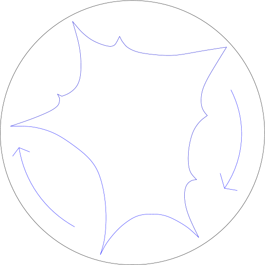
Figure 2: Small spikes propagating on a background of big spikes. The specific solution illustrated corresponds to the case $K=9$, $M=4$ and the curve shown in Figure 1.

The degeneration considered here is a generalisation of the limit considered in [18] (which corresponds to the case $M=0$) and our analysis of the component $\tilde{\Sigma}_{1}$ closely follows this reference. In particular we find that the period conditions for $\tilde{\Sigma}_{1}$ can be solved explicitly and the resulting curve precisely coincides with that of a classical $SL(2,\mathbb{R})$ Heisenberg spin chain of length $K-M$. Further, the semiclassical spectrum of string states corresponding to this sector coincides with the semiclassical spectrum of the spin chain. The same chain emerges directly in the analysis of string solutions with $K-M$ large spikes [19]. As worked out in detail in [19], the spin degrees of freedom correspond to the localised worldsheet Noether charges at each cusp of the string. Further, the moduli of $\tilde{\Sigma}_{1}$ correspond directly to the angular positions of the large spikes.

The main new ingredient in the present analysis is the new sectors with $M>0$ where there are $M$ additional simple poles in the quasi-momentum $dp$ on $\tilde{\Sigma}_{2}$. The poles arise in a standard way from the collision of branch points in the spectral data and are naturally associated with solitons propagating on the string. We will derive the corresponding semiclassical spectrum of string states and obtain a detailed match to the properties of the small spikes described above. In particular, we reproduce the dispersion relation (4). The resulting picture of the general large-$S$ state described by the curve $\Sigma$ is of $M$ small spikes propagating on the background provided by $K-M$ large spikes. A generic solution of this type is illustrated in Figure 2. The degeneration of the curve shown in Figure 1 corresponds to the decoupling of these two branches of the spectrum as $S\rightarrow\infty$.

The remainder of the paper is organised as follows. In the next section we review the basic set-up of the finite gap formalism for strings on $AdS_{3}\times S^{1}$. In Section 3 we consider the $S\rightarrow\infty$ limit of a generic $K$-gap string solution with $AdS$ angular momentum $S$, in particular we review the analysis of [18] which leads to a precise identification of the dynamics of large spikes with that of the classical gauge theory spin chain. We then generalise this analysis to include configurations corresponding to small spikes. We derive the dispersion relation for small spikes directly from the corresponding limit of the spectral curve. Some details of the calulation are relegated to an appendix.

2 The finite gap construction

We begin by focusing on classical bosonic string theory on $AdS_{3}\times S^{1}$. This is a sub-sector of classical string theory on the full $AdS_{5}\times S^{5}$ geometry which contains in particular the string duals to the $sl(2)$ sector operators of the form (1). Here the $U(1)$ R-charge $J$ of the gauge theory corresponds to momentum in the $S^{1}$ direction and the conformal spin $S$ corresponds to angular momentum in $AdS_{3}$. The string energy $\Delta$ corresponds to translations of the global time in $AdS_{3}$.

The simplest string solution is the so-called BMN groundstate: a pointlike string orbiting $S^{1}$ at the speed of light. This corresponds to the ferromagnetic groundstate of the dual gauge theory spin chain and has exact energy $\Delta=J$.

We introduce string worldsheet coordinates $\sigma\sim\sigma+2\pi$ and $\tau$ and the corresponding lightcone coordinates $\sigma_{\pm}=(\tau\pm\sigma)/2$ and we define lightcone derivatives $\partial_{\pm}=\partial_{\tau}\pm\partial_{\sigma}$. The space-time coordinates correspond to fields on the string worldsheet: we introduce $\phi(\sigma,\tau)\in S^{1}$ and parametrize $AdS_{3}$ with a group-valued field $g(\sigma,\tau)\in SU(1,1)\simeq AdS_{3}$. The $SU(1,1)_{R}\times SU(1,1)_{L}$ isometries of $AdS_{3}$ correspond to left and right group multiplication. The Noether current corresponding to right multiplication is $j_{\pm}=g^{-1}\partial_{\pm}g$. Following [25], we work in static, conformal gauge with a flat worldsheet metric and set,

$$\phi(\sigma,\tau) = \frac{J}{\sqrt{\lambda}}\,\,\tau$$

In this gauge, the string action becomes that of the $SU(1,1)$ Principal Chiral model,

$$S_{\sigma} = \frac{\sqrt{\lambda}}{4\pi}\,\int_{0}^{2\pi}\,d\sigma\,\frac{1}{2}{\rm tr}_{2}\left[j_{+}j_{-}\right]$$ (6)

As usual we expect a string moving in four spacetime dimensions to have two transverse degrees of freedom. Expanding around the BMN groundstate solution described above, we find two oscillation modes of equal mass carrying charges $S=\pm 1$. This is the usual transverse spectrum of the $AdS_{5}\times S^{5}$ string restricted to a bosonic $AdS_{3}\times S^{1}$ subspace. The two modes are dual to magnons of the gauge theory spin chain and correspond to insertions of light-cone covariant derivatives $\mathcal{D}_{+}$ and $\mathcal{D}_{-}$ in the BMN groundstate operator. The former excitations correspond to the $sl(2)$ sector operators identified above. The lightcone derivative $\mathcal{D}_{-}$ also generates a closed subsector of operators described by a Heisenberg spin at one loop, but operators containing both types of excitation do not form a closed subsector.

The equations of motion corresponding to (6) are integrable by virtue of their equivalence to the consistency conditions for the auxiliary linear problem,

$$\left[\partial_{\sigma}\,\,+\,\,\frac{1}{2}\left(\frac{j_{+}}{1-x}\,\,-\,\,\frac{j_{-}}{1+x}\right)\right]\cdot\vec{\Psi} = 0$$

$$\left[\partial_{\tau}\,\,+\,\,\frac{1}{2}\left(\frac{j_{+}}{1-x}\,\,+\,\,\frac{j_{-}}{1+x}\right)\right]\cdot\vec{\Psi} = 0$$

where $x\in\mathbb{C}$ is a complex spectral parameter. String motion is also subject to the Virasoro constraint,

$$\frac{1}{2}{\rm tr}_{2}\left[j_{\pm}^{2}\right] = -\frac{J^{2}}{\lambda}$$

Classical integrability of string theory on $AdS_{3}\times S^{1}$ follows from the construction of the monodromy matrix [4],

$$\Omega\left[x;\tau\right] = \,\,\mathcal{P}\,\,\exp\left[\frac{1}{2}\int_{0}^{2\pi}\,d\sigma\,\,\left(\frac{j_{+}}{x-1}\,\,+\,\,\frac{j_{-}}{x+1}\right)\right]\,\,\,\,\in\,\,\,\,SU(1,1)$$

whose eigenvalues $w_{\pm}=\exp(\pm i\,p(x))$ are $\tau$-independent for all values of the spectral parameter $x$. It is convenient to consider the analytic continuation of the monodromy matrix $\Omega[x;\tau]$ and of the quasi-momentum $p(x)$ to complex values of $x$. In this case $\Omega$ will take values in $SL(2,\mathbb{C})$ and appropriate reality conditions must be imposed to recover the physical case.

The eigenvalues $w_{\pm}(x)$ are two branches of an analytic function defined on the spectral curve,

$$\Sigma_{\Omega}\,\,:\qquad{}\qquad{}{\rm det}\left(w\mathbb{I}\,\,-\,\,\Omega[x;\tau]\right)\,\,=\,\,w^{2}\,\,-\,\,2\cos p(x)\,w\,\,+\,\,1 = 0\qquad{}w,\,\,x\in\mathbb{C}$$

This curve corresponds to a double cover of the complex $x$-plane with branch points at the simple zeros of the discriminant $D=4\sin^{2}p(x)$. In addition the monodromy matrix defined above is singular at the points above $x=\pm 1$. Using the Virasoro constraint, one may show that $p(x)$ has simple poles at these points,

$$p(x) \sim \frac{\pi J}{\sqrt{\lambda}}\frac{1}{(x\pm 1)}\,+\,O\left((x\pm 1)^{0}\right)$$ (7)

as $x\rightarrow\mp 1$. Hence the discriminant $D$ has essential singularities at $x=\pm 1$ and $D$ must therefore have an infinite number of zeros which accumulate at these points. Formally we may represent the discriminant as a product over its zeros and write the spectral curve as

$$\Sigma_{\Omega}\,\,:\qquad{}\qquad{}{y}^{2}_{\Omega}\,\,=\,\,4\sin^{2}p(x) = \prod_{j=1}^{\infty}\left(x-x_{i}\right)$$

For generic solutions the points $x=x_{i}$ are distinct and the curve ${\Sigma}_{\Omega}$ has infinite genus.

In order to make progress it is necessary to focus on solutions for which the discriminant has only a finite number $2K$ of simple zeros and the spectral curve ${\Sigma}_{\Omega}$ has finite genus. The infinite number of additional zeros of the discriminant $D$ must then have multiplicity two or higher. These are known as finite gap solutions. In this case, $dp$ is a meromorphic differential on the hyperelliptic curve of genus $g=K-1$ which is obtained by removing the double points of $\hat{\Sigma}$ (see [26]).

Finite-gap review

The construction of solutions to the string equations of motion for this system is given in [25] and reviewed in [18]. Solutions are labelled by the number $K\geq 0$ of gaps in the spectrum of the auxiliary linear problem. The $K$-gap solutions are characterised by a hyperelliptic curve $\Sigma$ of genus $K-1$ and a meromorphic differential $dp$ on $\Sigma$ with prescribed singularities and asymptotics which will be reviewed below. For simplicity we will focus on the case of even $K$.

In the following we will also focus on curves where all the branch points lie on the real axis and outside the interval $[-1,+1]$. This corresponds to string solutions where only classical oscillator modes which carry positive spin are activated. In other words, only the transverse modes of the string with angular momentum $S=+1$ are excited. In the dual gauge theory these solutions are believed to correspond to operators of the form (1) where only the covariant derivative $\mathcal{D}_{+}$, which carries positive spin, appears [25].

We label the branch points of the curve according to,

$$\Sigma\,\,:\qquad{}y^{2} = \prod_{i=1}^{K}\left(x-x^{(i)}_{+}\right)\left(x-x^{(i)}_{-}\right)$$ (8)

with the ordering,

$$x_{-}^{(K)}\,\,\leq\,\,x_{-}^{(K-1)} \ldots \leq x_{-}^{(1)}\,\,\leq-1$$

$$x_{+}^{(K)}\,\,\geq\,\,x_{+}^{(K-1)} \ldots \geq x_{+}^{(1)}\,\,\geq+1$$

The branch points are joined in pairs by cuts $C^{\pm}_{I}$, $I=1,2,\ldots,K/2$ as shown in Figure 3. We also define a standard basis of one-cycles, $\mathcal{A}^{\pm}_{I}$, $\mathcal{B}^{\pm}_{I}$. Here $\mathcal{A}^{\pm}_{I}$ encircles the cut $C^{\pm}_{I}$ on the upper sheet in an anti-clockwise direction and $\mathcal{B}^{\pm}_{I}$ runs from the point at infinity on the upper sheet to the point at infinity on the lower sheet passing through the cut $C^{\pm}_{I}$, as shown in Figure 4.

\psfrag{x}{\footnotesize{$x$}}\psfrag{m1}{\footnotesize{$-1$}}\psfrag{p1}{\footnotesize{$+1$}}\psfrag{C1m}{\footnotesize{$C_{1}^{-}$}}\psfrag{C1p}{\footnotesize{$C_{1}^{+}$}}\psfrag{C1k}{\footnotesize{$C_{K/2}^{-}$}}\psfrag{C1j}{\footnotesize{$C_{K/2}^{+}$}}\psfrag{a}{\footnotesize{$x^{(K)}_{-}$}}\psfrag{b}{\footnotesize{$x^{(K-1)}_{-}$}}\psfrag{c}{\footnotesize{$x^{(2)}_{-}$}}\psfrag{d}{\footnotesize{$x^{(1)}_{-}$}}\psfrag{e}{\footnotesize{$x^{(1)}_{+}$}}\psfrag{f}{\footnotesize{$x^{(2)}_{+}$}}\psfrag{g}{\footnotesize{$x^{(K-1)}_{+}$}}\psfrag{h}{\footnotesize{$x^{(K)}_{+}$}}\includegraphics[width=284.52756pt]{Sfig1.eps}

Figure 3: The cut $x$-plane corresponding to the curve $\Sigma$

\psfrag{AI}{\footnotesize{$\mathcal{A}^{\pm}_{I}$}}\psfrag{BI}{\footnotesize{$\mathcal{B}^{\pm}_{I}$}}\psfrag{CI}{\footnotesize{$C^{\pm}_{I}$}}\psfrag{Ip}{\footnotesize{$\infty^{+}$}}\psfrag{Im}{\footnotesize{$\infty^{-}$}}\includegraphics[width=284.52756pt]{Sfig2.eps}

Figure 4: The cycles on $\Sigma$. The index $I$ runs from $1$ to $K/2$.

The meromorphic differential $dp$ on $\Sigma$ has second-order poles at the points above $x=+1$ and $x=-1$ on $\Sigma$ whose coefficients encode the $S^{1}$ angular momentum of the solution. On the top sheet we have,

$$dp \longrightarrow -\frac{\pi J}{\sqrt{\lambda}}\frac{dx}{(x\pm 1)^{2}}\,\,+\,\,O\left((x\pm 1)^{0}\right)$$ (9)

as $x\rightarrow\mp 1$.

There are also two second-order poles at the points $x=\mp 1$ on the lower sheet related by the involution $dp\rightarrow-dp$. The value of the Noether charges $\Delta$ and $S$ is encoded in the asymptotic behaviour of $dp$ near the points $x=0$ and $x=\infty$ on the top sheet,

$$dp \longrightarrow -\frac{2\pi}{\sqrt{\lambda}}\,\,\left(\Delta\,+\,S\right)\,\,\frac{dx}{x^{2}}\qquad{}{\rm as}\,\,\,\,x\rightarrow\infty$$ (10)

$$dp \longrightarrow -\frac{2\pi}{\sqrt{\lambda}}\,\,\left(\Delta\,-\,S\right)\,\,dx\qquad{}{\rm as}\,\,\,\,x\rightarrow 0$$ (11)

For a valid semiclassical description, the conserved charges $J$, $S$ and $\Delta$ should all be $O(\sqrt{\lambda})$ with $\sqrt{\lambda}>>1$.

In addition to the above relations, the closed string boundary condition imposes $2K$ normalisation conditions on $dp$,

$$\oint_{\mathcal{A}^{\pm}_{I}}\,dp\,\,=\,\,0 \oint_{\mathcal{B}^{\pm}_{I}}\,dp\,\,=\,\,2\pi n^{\pm}_{I}$$ (12)

with $I=1,2,\ldots,K/2$. The integers $n^{\pm}_{I}$ correspond to the mode numbers of the string. In the following we will assign the mode numbers so as to pick out the $K$ lowest modes of the string which carry positive angular momentum, including both left and right movers. This is accomplished by setting $n^{\pm}_{I}=\pm I$ for $I=1,\ldots,K/2$.

To find the spectrum of classical string solutions we must first construct the meromorphic differential $dp$ with the specified pole behaviour (9). The most general possible such differential has the form,

$$dp = dp_{1}\,\,+\,\,dp_{2}\,\,=\,\,-\frac{dx}{y}\left[f(x)\,\,+\,\,g(x)\right]$$ (13)

$$f(x) = \sum_{\ell=0}^{K-2}\,\,C_{\ell}\,x^{\ell}$$

$$g(x) = \frac{\pi J}{\sqrt{\lambda}}\left[\frac{y_{+}}{(x-1)^{2}}\,\,+\,\,\frac{y_{-}}{(x+1)^{2}}+\frac{y^{\prime}_{+}}{(x-1)}\,\,+\,\,\frac{y^{\prime}_{-}}{(x+1)}\right]$$

with $y_{\pm}=y(\pm 1)$ and

$$y^{\prime}_{\pm} = \left.\frac{dy}{dx}\right|_{x=\pm 1}$$

Here the second term $dp_{2}$ is a particular differential with the required poles and the first term $dp_{1}$ is a general holomorphic differential on $\Sigma$. The resulting curve $\Sigma$ and differential $dp$ depend on $3K-1$ undetermined parameters $\{x^{(i)}_{\pm},C_{\ell}\}$ with $i=1,\ldots,K$, $\ell=0,1,\ldots,K-2$. We then obtain $2K$ constraints on these parameters from the normalisation equations (12), leaving us with a $K-1$ dimensional moduli space of solutions [25]. A significant difficulty with this approach is that the normalisation conditions are transcendental and cannot be solved in closed form.

A convenient parametrisation for the moduli space is given in terms of the $K$ filling fractions,

$$\mathcal{S}^{\pm}_{I} = -\frac{1}{2\pi i}\,\cdot\,\frac{\sqrt{\lambda}}{4\pi}\,\,\oint_{\mathcal{A}^{\pm}_{I}}\,\left(x\,+\,\frac{1}{x}\right)\,dp$$ (14)

with $I=1,\ldots,K/2$, subject to the level matching constraint,

$$\sum_{I=1}^{K/2}\,\,\left(n^{+}_{I}\mathcal{S}^{+}_{I}\,\,+\,\,n^{-}_{I}\mathcal{S}^{-}_{I}\right) = 0$$ (15)

Here the total $AdS$ angular momentum is given as

$$S = \sum_{I=1}^{K/2}\,\left(\mathcal{S}^{+}_{I}\,\,+\,\,\mathcal{S}^{-}_{I}\right)$$

and is regarded as one of the moduli of the solution. The significance of the filling fractions is that they constitute a set of normalised action variables for the string. They are canonically conjugate to angles $\varphi_{I}\in[0,2\pi]$ living on the Jacobian torus $\mathcal{J}(\Sigma)$. Evolution of the string solution in both worldsheet coordinates, $\sigma$ and $\tau$, corresponds to linear motion of these angles [26].

The constraints described above uniquely determine $(\Sigma,dp)$ for given values of $\mathcal{S}^{\pm}_{I}$, and one may then extract the string energy from the asymptotics (10,11) which imply,

$$\Delta\,+\,S = \frac{\sqrt{\lambda}}{2\pi}\,C_{K-2}$$

$$\Delta\,-\,S = \frac{\sqrt{\lambda}}{2\pi}\,\frac{C_{0}}{y(0)}\,\,+\,\,\frac{J}{2y(0)}\left(y_{+}+y_{-}-y^{\prime}_{+}+y^{\prime}_{-}\right)$$

In this way, one obtains a set of transcendental equations which determine the string energy as a function of the filling fractions,

$$\Delta = \Delta\left[\mathcal{S}^{+}_{1},\mathcal{S}^{-}_{1},\ldots,\mathcal{S}^{+}_{K/2},\mathcal{S}^{-}_{K/2}\right]$$

The leading order semiclassical spectrum of the string is obtained by imposing the Bohr-Sommerfeld conditions which impose the integrality of the filling fractions [26, 27]: $\mathcal{S}^{\pm}_{I}\in\mathbb{Z}$, $I=1,2,\ldots,K/2$.

Finally we define the quasi-momentum as the abelian integral of the differential $dp$,

$$p(x) = \int_{\infty^{+}}^{x}\,\,dp$$ (16)

where $\infty^{+}$ indicates complex infinity on the upper sheet.

3 The large spin limit

Our goal now is to investigate the large spin limit of the finite gap construction and in particular focus on excitations around the long spinning string solution. Here we will repeat and extend the analysis of [18]. To this end we label the branch points in the following way,

$$x^{(i)}_{\pm} = b\qquad{}\qquad{}\,\,\,i=1$$

$$= b^{(i-1)}_{\pm}\qquad{}\,\,\,\,\,\,\,\,i=2,\ldots,M+1$$

$$= a^{(i-M-1)}_{\pm}\qquad{}\,\,\,i=M+2,\ldots,K$$

where $M$ must be even. To obtain large spin, it is necessary to scale the coordinates of at least two of the branch points linearly with $S$ as $S\rightarrow\infty$. Here we will take a generic limit of this kind where the “$a$” branch points introduced above scale with $S$ while the “$b$” branch points are held fixed. We introduce a scaling parameter $\rho$ and set

$$a^{(j)}_{\pm} = \rho\tilde{a}_{\pm}^{(j)}$$

for $j=1,2,\ldots,K-M-1$ and take the limit $\rho\rightarrow\infty$ with $\tilde{a}^{(j)}_{\pm}$, $b^{(j)}_{\pm}$ and $b$ held fixed. Thus we are dividing the branch points into “large” and “small”. This is a generalisation of the limit considered in [18] (which in the present notation corresponds to $M=0$) and we will draw heavily on the results of this reference.

The key point is that the limit must be taken in such a way that the conditions on the periods of the differential $dp$ are preserved. As explained in [18] the scaling leads to a very specific degeneration of the spectral curve $\Sigma$ into two components;

$$\Sigma \longrightarrow \tilde{\Sigma}_{1}\cup\tilde{\Sigma}_{2}$$

The two components $\tilde{\Sigma}_{1}$ and $\tilde{\Sigma}_{2}$ correspond to the “large” and “small” branch points respectively. The curves are given explicitly as

$$\tilde{\Sigma}_{1}\,\,:\qquad{}\tilde{y}^{2}_{1} = \prod_{i=1}^{K-M-1}\left(\tilde{x}-\tilde{a}^{(i)}_{+}\right)\left(\tilde{x}-\tilde{a}^{(i)}_{-}\right)\>,$$

where $\tilde{x}=x/\rho$ is the rescaled spectral parameter, and

$$\tilde{\Sigma}_{2}\,\,:\qquad{}\tilde{y}^{2}_{2} = (x^{2}\,-\,b^{2})\prod_{i=1}^{M}\left(x-b^{(i)}_{+}\right)\left(x-b^{(i)}_{-}\right)$$

These two surfaces have genus $K-M-2$ and $M$ respectively. At this point we have not yet imposed the period conditions (12). In the following we will see that these two surfaces describe the dynamics of “large” and “small” spikes respectively. The differential $dp$ also decomposes into differentials $d\tilde{p}_{1}$ and $d\tilde{p}_{2}$ on each of these curves,

$$dp \longrightarrow d\tilde{p}_{1}\,\,\,\,+\,\,\,\,d\tilde{p}_{2}$$

Review of the simple case $M=0$

We begin by briefly reviewing the case considered in [18] which corresponds to $M=0$. The corresponding degeneration of the spectral curve is illustrated in Figure 5.

\psfrag{S1}{\footnotesize{$\Sigma$}}\psfrag{S2}{\footnotesize{$\tilde{\Sigma}_{2}$}}\psfrag{Ip}{\footnotesize{$\infty^{+}$}}\psfrag{Im}{\footnotesize{$\infty^{-}$}}\includegraphics[width=284.52756pt]{SGMfig3b.eps}

\psfrag{S1}{\footnotesize{$\Sigma$}}\psfrag{S2}{\footnotesize{$\tilde{\Sigma}_{2}$}}\psfrag{Ip}{\footnotesize{$\infty^{+}$}}\psfrag{Im}{\footnotesize{$\infty^{-}$}}\psfrag{S1}{\footnotesize{$\tilde{\Sigma}_{1}$}}\psfrag{S2}{\footnotesize{$\tilde{\Sigma}_{2}$}}\includegraphics[width=284.52756pt]{SGMfig3.eps}

Figure 5: The degeneration $\Sigma\rightarrow\tilde{\Sigma}_{1}\cup\tilde{\Sigma}_{2}$. The four singular points $\pm 1^{\pm}$ are marked with crosses on the curve.

The key point is that the differential $d\tilde{p}_{1}$ on $\tilde{\Sigma}_{1}$ has only simple poles and it is then possible to solve the conditions on the periods of this differential to find an explict parametrization of the curve. The relevant formulae are,

$$\tilde{\Sigma}_{1}\>\>:\qquad\tilde{y}_{1}^{2}=\prod_{i=1}^{K-1}\left(\tilde{x}-\tilde{a}^{(i)}_{+}\right)\left(\tilde{x}-\tilde{a}^{(i)}_{-}\right)$$ (17)

and

$$d\tilde{p}_{1}=-i\frac{d\tilde{x}}{\tilde{x}^{2}}\frac{\mathbb{P}^{\prime}_{K}\left(\frac{1}{\tilde{x}}\right)}{\sqrt{\mathbb{P}_{K}^{2}\left(\frac{1}{\tilde{x}}\right)-4}}$$ (18)

with

$$\mathbb{P}_{K}\left(\frac{1}{\tilde{x}}\right)=2+\frac{\tilde{q}_{2}}{\tilde{x}^{2}}+\frac{\tilde{q}_{3}}{\tilde{x}^{3}}+\ldots+\frac{\tilde{q}_{K}}{\tilde{x}^{K}}\>,$$ (19)

The curve coincides with the curve of a classical $SL(2,\mathbb{R})$ spin chain of length $K$ and $d\tilde{p}_{1}$ is precisely the quasi-momentum of this system. The $K-1$ remaining moduli $\tilde{q}_{i}$ are the conserved charges of the spin chain.

It is also straightforward to find the limiting form of the second component and the corresponding differential,

$$\tilde{\Sigma}_{2}\,\,:\qquad{}\tilde{y}^{2}_{2} = (x^{2}\,-\,b^{2})$$

and

$$d\tilde{p}_{2} = -\,\frac{i\pi J}{\sqrt{\lambda}}\left[\sqrt{b^{2}-1}\left(\frac{1}{(x-1)^{2}}\,+\,\frac{1}{(x+1)^{2}}\right)\,\,-\,\,\frac{1}{\sqrt{b^{2}-1}}\left(\frac{1}{(x-1)}\,-\,\frac{1}{(x+1)}\right)\,\right]\,\,\frac{dx}{\tilde{y}_{2}}$$ (20)

$$\qquad-\frac{K}{i}\frac{dx}{\tilde{y}_{2}}$$

\psfrag{S1}{\footnotesize{$\Sigma$}}\psfrag{S2}{\footnotesize{$\tilde{\Sigma}_{2}$}}\includegraphics[width=284.52756pt]{SGMfig6b.eps}

\psfrag{S1}{\footnotesize{$\Sigma$}}\psfrag{S2}{\footnotesize{$\tilde{\Sigma}_{2}$}}\psfrag{S1}{\footnotesize{$\tilde{\Sigma}_{1}$}}\psfrag{S2}{\footnotesize{$\tilde{\Sigma}_{2}$}}\includegraphics[width=284.52756pt]{SGMfig6.eps}

Figure 6: The “extra” cycle $\mathcal{A}^{+}_{K/2}$ gives rise to the matching condition.

Of the period conditions on the original surface $\Sigma$, all but one become period conditions on the differential $d\tilde{p}_{1}$ which are solved explicitly in (18). The “extra” period becomes a sum of chains on both components. The corresponding normalisation equation gives rise to a matching condition which relates the moduli of the two component surfaces and takes the form,

$$\sqrt{b^{2}-1} = \frac{2\pi J}{\sqrt{\lambda}}\,\times\,\frac{1}{K\log\left(\rho\tilde{q}_{K}^{1/K}\right)}$$ (21)

In the $\rho\rightarrow\infty$ limit, the conserved charges have the behaviour,

$$\Delta\,+\,S \simeq \frac{\sqrt{\lambda}}{2\pi}\sqrt{-\tilde{q}_{2}}\,\,\rho\qquad{}\rightarrow\,\,\,\,\infty$$

$$\Delta\,-\,S \simeq -\frac{\sqrt{\lambda}}{2\pi}\,\,\frac{K}{b}\,\,\,+\,\,\,\frac{J}{b}\left(\sqrt{b^{2}-1}\,+\,\frac{1}{\sqrt{b^{2}-1}}\right)$$ (22)

up to corrections which vanish as $\rho\rightarrow\infty$. The behaviour of the inner branch points $x=\pm b$ in this limit is determined by the matching condition (21). Thus, as the scaling parameter $\rho$ goes to infinity, $b\rightarrow 1$ and the inner branch points approach the punctures at the points $x=\pm 1$. Comparing (21) with (22) we find the limiting behaviour,

$$\sqrt{b^{2}-1} \simeq \frac{J}{\Delta-S}$$

Finally taking account of this limit in (20) we find the limiting form of the quasi-momentum,

$$\left.d\tilde{p}_{2}\right|_{M=0} \simeq \frac{2\pi i}{\sqrt{\lambda}}\,(\Delta-S)\,\,\frac{dx}{(x^{2}-1)^{\frac{3}{2}}}$$ (23)

This is the leading contribution to the quasi-momentum in the limit $S\rightarrow\infty$ up to contributions which are supressed by inverse powers of $\log S$, while the anomalous dimension is given by:

$$\Delta-S\simeq\frac{\sqrt{\lambda}}{2\pi}\left[K\log S+\log\left(\frac{\tilde{q}_{K}}{(-\tilde{q}_{2})^{K/2}}\right)+\mathrm{const.}\right]+\ldots$$ (24)

where the constant is moduli-independent. This moduli-dependent term in this expression coincides with the nearest-neighbour Hamiltonian of the $SL(2,\mathbb{R})$ spin chain.

The main result of the analysis of [18] is that the semiclassical spectrum of string theory on $AdS_{3}\times S^{1}$ in the particular limit described above is captured by the classical spin chain. In [19], approximate solutions corresponding to this spectrum were constructed. The solutions include $K$ large spikes with angular positions which can be related to the moduli $\tilde{q}_{i}$ appearing in the spin chain curve. Our next objective is to generalise this analysis to the more general limit discussed above with $M>0$. Thus we will include “small” branch points and we will see that they correspond to the contributions of small spikes.

The general case $M$ even

The main difference from the previous case is the fact that now $2M+2$ “small” branch points (located at $x=b^{(j)}_{\pm}$, $j=1,\ldots,M$, and at the usual $x=\pm b$) migrate to $\tilde{\Sigma}_{2}$ as $\rho\to\infty$. Thus, as explained above, after the factorisation this surface has, in principle, genus $M$, although we will later see that this will reduce to $1$ due to cut collisions. $\tilde{\Sigma}_{1}$, on the other hand, has now genus $K-M-2$ and contains all the “large” branch points. The extra cuts transferred to $\tilde{\Sigma}_{2}$ make the analysis more difficult on that surface.

First of all, it is convenient to rearrange the cycles on $\Sigma$ before we take the large-$S$ limit. The new equivalent configurations of the A-cycles and of the B-cycles are shown in Fig. 7(a) and 8(a) respectively. In particular, we define $\hat{\mathcal{A}}_{I}^{\pm}=\sum_{J=I}^{K/2}\mathcal{A}_{J}^{\pm}$, for $I=(K-M)/2,\ldots,K/2$ and $\hat{\mathcal{A}}_{0}=\sum_{J=(K-M)/2}^{K/2}(\mathcal{A}_{J}^{+}+\mathcal{A}_{J}^{-})$, together with $\hat{\mathcal{B}}=\mathcal{B}_{(K-M)/2}^{-}-\mathcal{B}_{(K-M)/2}^{+}$, $\hat{\mathcal{B}}_{I}^{-}=\mathcal{B}_{I-1}^{-}-\mathcal{B}_{I}^{-}$ and $\hat{\mathcal{B}}_{I}^{+}=\mathcal{B}_{I}^{+}-\mathcal{B}_{I-1}^{+}$, for $I=(K-M)/2+1,\ldots,K/2$.

Basically, we have modified in a suitable way only the cycles associated with those cuts which will move to $\tilde{\Sigma}_{2}$ in the limit $\rho\to\infty$. A consistent set of period conditions on $\Sigma$ is then:

$$\oint_{\mathcal{A}_{I}^{\pm}}dp=0 \oint_{\mathcal{B}_{I}^{\pm}}dp=2\pi n_{I}^{\pm}=\pm 2\pi I\qquad\textrm{for }I=1,\ldots,\frac{K-M}{2}-1$$

$$\oint_{\tilde{\mathcal{A}}_{0}}dp=0 \oint_{\hat{\mathcal{B}}}dp=-2\pi(K-M)$$

$$\oint_{\hat{\mathcal{A}}_{\frac{K-M}{2}}^{+}}dp=0 \oint_{\mathcal{B}_{\frac{K-M}{2}}^{+}}dp=\pi(K-M)$$

$$\oint_{\hat{\mathcal{A}}_{J}^{\pm}}dp=0 \oint_{\hat{\mathcal{B}}_{J}^{\pm}}dp=2\pi\qquad\textrm{for }I=\frac{K-M}{2}+1,\ldots,K/2$$ (25)

Fig. 7(b) and 8(b) show which cycles survive on $\tilde{\Sigma}_{1}$ (identified as the region close to the branch points $a^{(j)}_{\pm}$) when we take $\rho$ to infinity, while Fig. 7(c) and 8(c) show the configuration for $\tilde{\Sigma}_{2}$ (corresponding to the region close to the $b^{(j)}_{\pm}$) in the same limit.

\psfrag{a}{\footnotesize{(a)}}\psfrag{b}{\footnotesize{(b)}}\psfrag{c}{\footnotesize{(c)}}\psfrag{a1}{\footnotesize{$\mathcal{A}_{\frac{K-M}{2}-1}^{+}$}}\psfrag{a2}{\footnotesize{$\mathcal{A}_{1}^{+}$}}\psfrag{a3}{\footnotesize{$\mathcal{A}_{\frac{K-M}{2}-1}^{-}$}}\psfrag{a4}{\footnotesize{$\mathcal{A}_{1}^{-}$}}\psfrag{a5}{\footnotesize{$\tilde{\mathcal{A}}_{0}$}}\psfrag{a6}{\footnotesize{$\hat{\mathcal{A}}_{\frac{K}{2}-1}^{-}$}}\psfrag{a7}{\footnotesize{$\hat{\mathcal{A}}_{\frac{K}{2}}^{-}$}}\psfrag{a8}{\footnotesize{$\hat{\mathcal{A}}_{\frac{K-M}{2}}^{+}$}}\psfrag{a9}{\footnotesize{$\hat{\mathcal{A}}_{\frac{K}{2}-1}^{+}$}}\psfrag{a10}{\footnotesize{$\hat{\mathcal{A}}_{\frac{K}{2}}^{+}$}}\includegraphics[width=433.62pt]{Acycles.eps}

Figure 7: (a) The rearranged A-cycle configuration on $\Sigma$. (b) The A-cycles on $\tilde{\Sigma}_{1}$; the marked point indicates the simple pole at $x=0$. (c) The A-cycles on $\tilde{\Sigma}_{2}$; the marked points indicate the double poles at $x=\pm 1$. All dashed lines extend to infinity along the real axis.

\psfrag{a}{\footnotesize{(a)}}\psfrag{b}{\footnotesize{(b)}}\psfrag{c}{\footnotesize{(c)}}\psfrag{b1}{\footnotesize{$\mathcal{B}_{1}^{-}$}}\psfrag{b2}{\footnotesize{$\mathcal{B}_{\frac{K-M}{2}-1}^{-}$}}\psfrag{b3}{\footnotesize{$\mathcal{B}_{1}^{+}$}}\psfrag{b4}{\footnotesize{$\mathcal{B}_{\frac{K-M}{2}-1}^{+}$}}\psfrag{b5}{\footnotesize{$\mathcal{B}_{\frac{K-M}{2}}^{+}$}}\psfrag{b6}{\footnotesize{$\hat{\mathcal{B}}$}}\psfrag{b7}{\footnotesize{$\hat{\mathcal{B}}_{\frac{K}{2}}^{-}$}}\psfrag{b8}{\footnotesize{$\hat{\mathcal{B}}_{\frac{K}{2}-1}^{-}$}}\psfrag{b9}{\footnotesize{$\hat{\mathcal{B}}_{\frac{K-M}{2}+1}^{-}$}}\psfrag{b10}{\footnotesize{$\hat{\mathcal{B}}_{\frac{K}{2}}^{+}$}}\psfrag{b11}{\footnotesize{$\hat{\mathcal{B}}_{\frac{K}{2}-1}^{+}$}}\psfrag{b12}{\footnotesize{$\hat{\mathcal{B}}_{\frac{K-M}{2}+1}^{+}$}}\includegraphics[width=433.62pt]{Bcycles.eps}

Figure 8: (a) The rearranged B-cycle configuration on $\Sigma$. Dashed blue lines indicate paths on the lower sheet throughout the picture. (b) The B-cycles on $\tilde{\Sigma}_{1}$; the marked point indicates the simple pole at $x=0$. (c) The B-cycles on $\tilde{\Sigma}_{2}$; the marked points indicate the double poles at $x=\pm 1$. The black dashed lines extend to infinity along the real axis.

As in the previous case, the spectral problem reduces to two (almost) separate problems on $\tilde{\Sigma}_{1}$ and $\tilde{\Sigma}_{2}$. On the first surface

$$\tilde{\Sigma}_{1}\>\>:\qquad\tilde{y}_{1}^{2}=\prod_{k=1}^{K-M-1}(\tilde{x}-\tilde{a}^{(k)}_{+})(\tilde{x}-\tilde{a}^{(k)}_{-})$$ (26)

we have the following limiting form of the differential

$$d\tilde{p}_{1}=-\frac{d\tilde{x}}{\tilde{y}_{1}}\sum_{l=M}^{K-2}\tilde{C}_{l}\tilde{x}^{l-M-1}$$ (27)

where $\tilde{x}=x/\rho$ as usual and we have rescaled the parameters $C_{l}$ as follows:

$$C_{l}=\left\{\begin{array}[]{ll}\tilde{C}_{l}\,\rho^{K-l-1}\>,&\textrm{for }l\geq M\\ \tilde{C}_{l}\,\rho^{K-M-1}\>,&\textrm{for }l<M\end{array}\right.$$ (28)

This ensures that $d\tilde{p}_{1}$ has a simple pole at $\tilde{x}=0$ and that none of these parameters disappears from both $d\tilde{p}_{1}$ and $d\tilde{p}_{2}$ due to suppression by negative powers of $\rho$. As we can see from Figures 7(b) and 8(b), the differential is subject to the following period conditions, which are inherited from $\Sigma$ (25):

$$\oint_{\mathcal{A}_{I}^{\pm}}d\tilde{p}_{1}=0 \oint_{\mathcal{B}_{I}^{\pm}}d\tilde{p}_{1}=2\pi n_{I}^{\pm}=\pm 2\pi I\qquad\textrm{for }I=1,\ldots,\frac{K-M}{2}-1$$

$$\oint_{\tilde{\mathcal{A}}_{0}}d\tilde{p}_{1}=0 \oint_{\hat{\mathcal{B}}}d\tilde{p}_{1}=-2\pi(K-M)$$ (29)

$$\oint_{\mathcal{B}_{\frac{K-M}{2}}^{+}}d\tilde{p}_{1}=\pi(K-M)$$

On $\tilde{\Sigma}_{2}$, which is parametrised as

$$\tilde{\Sigma}_{2}\>\>:\qquad\tilde{y}_{2}^{2}=(x^{2}-b^{2})\prod_{i=1}^{M}(x-b^{(i)}_{+})(x-b^{(i)}_{-})\>,$$ (30)

we find instead

$$d\tilde{p}_{2}=-\frac{dx}{\tilde{Q}\tilde{y}_{2}}\sum_{l=0}^{M}\tilde{C}_{l}x^{l}-\frac{\pi J}{\sqrt{\lambda}}\left[\frac{\tilde{y}_{2}(1)}{(x-1)^{2}}+\frac{\tilde{y}_{2}(-1)}{(x+1)^{2}}+\frac{\tilde{y}^{\prime}_{2}(1)}{x-1}+\frac{\tilde{y}^{\prime}_{2}(-1)}{x+1}\right]\frac{dx}{\tilde{y}_{2}}$$ (31)

with $\tilde{Q}^{2}=\tilde{y}_{1}^{2}(0)$. The corresponding period conditions are given by:

$$\oint_{\hat{\mathcal{A}}_{J}^{\pm}}d\tilde{p}_{2}=0 \oint_{\hat{\mathcal{B}}_{J}^{\pm}}d\tilde{p}_{2}=2\pi\qquad\textrm{for }I=\frac{K-M}{2}+1,\ldots,K/2$$ (32)

as shown in Figures 7(c) and 8(c). Only one period condition from the original set (25) remains, namely:

$$\oint_{\hat{\mathcal{A}}_{\frac{K-M}{2}}^{+}}dp=0$$ (33)

which involves the only cycle that survives both on $\tilde{\Sigma}_{1}$ and on $\tilde{\Sigma}_{2}$. This constraint then provides a relationship between the two problems associated with these surfaces and we will therefore refer to it as the “matching condition”.

Explicit solution on $\tilde{\Sigma}_{1}$

The period conditions on the first surface can be solved explicitly exactly as explained in [18], the crucial point being once again that $d\tilde{p}_{1}$ only has a simple pole and no other singularities (apart from the branch points). We find:

$$d\tilde{p}_{1}=-i\frac{d\tilde{x}}{\tilde{x}^{2}}\frac{\mathbb{P}^{\prime}_{K-M}\left(\frac{1}{\tilde{x}}\right)}{\sqrt{\mathbb{P}_{K-M}^{2}\left(\frac{1}{\tilde{x}}\right)-4}}$$ (34)

where

$$\mathbb{P}_{K-M}\left(\frac{1}{\tilde{x}}\right)=2+\frac{\tilde{q}_{2}}{\tilde{x}^{2}}+\frac{\tilde{q}_{3}}{\tilde{x}^{3}}+\ldots+\frac{\tilde{q}_{K-M}}{\tilde{x}^{K-M}}$$ (35)

and the parameters $\tilde{q}_{j}$ are related to the $\tilde{C}_{l}$ through

$$\tilde{C}_{l}=-\frac{(K-l)\tilde{q}_{K-l}}{2\sqrt{-\tilde{q}_{2}}}$$ (36)

for $l=M,\ldots,K-2$.

As in the $M=0$ case, the spectral curve coincides with the curve of a classical $SL(2,\mathbb{R})$ spin chain, whose length is now $K-M$, and $d\tilde{p}_{1}$ is the differential of the corresponding quasi-momentum. The $K-M-1$ parameters $\tilde{q}_{j}$ are the moduli associated with the first surface after the factorisation and they also represent the conserved charges of the spin chain.

With reference to Figure 1, $\tilde{\Sigma}_{1}$ is the surface on the left-hand side of the bottom picture. Its main features are the $K-M-1$ branch cuts and the two singular contact points with $\tilde{\Sigma}_{2}$, which are located at $\tilde{x}=0^{\pm}$ (where $0^{+}$ lies on the top sheet, while $0^{-}$ lies on the bottom sheet).

Explicit solution on $\tilde{\Sigma}_{2}$

The procedure on this surface is a bit more involved than it was in the previous case.

By imposing the matching condition (33) (which will be discussed in appendix A) at leading order, it is possible to show that, as in the $M=0$ case, the two innermost branch points on $\tilde{\Sigma}_{2}$ have to collide with the neighbouring double poles, i.e. that $b\to 1$ so that:

$$\frac{1}{\sqrt{1-b^{2}}}\sim i\log\epsilon$$ (37)

where $\epsilon=1/\rho$.

We now focus our attention on the A-cycle conditions on $\tilde{\Sigma}_{2}$. First of all, we notice that, due to the fact that the double poles at $x=\pm 1$ have vanishing residues, $b\to 1$ does not imply that the contours are pinched at these singularities. In fact, even before the limit $\rho\to\infty$ is taken, we are free to rearrange the cycles so that they cross the real axis along the interval $-1<x<1$, where clearly there can be no pinching (see Fig. 9(a)). It then follows that, even in the $\rho\to\infty$ limit, the contours $\hat{\mathcal{A}}_{I}^{\pm}$ do not touch any of the singularities of the differential. Therefore, the only diverging contribution the integrals receive comes from the factor $1/\sqrt{1-b^{2}}$ inside the integrand. For them to vanish, a second infinite contribution must arise in order to compensate.

\psfrag{a}{\footnotesize{(a)}}\psfrag{b}{\footnotesize{(b)}}\psfrag{a1}{\footnotesize{$\hat{\mathcal{A}}_{\frac{K}{2}}^{+}$}}\psfrag{a2}{\footnotesize{$\hat{\mathcal{A}}_{\frac{K}{2}-1}^{+}$}}\psfrag{a3}{\footnotesize{$\hat{\mathcal{A}}_{\frac{K-M}{2}+1}^{+}$}}\psfrag{a4}{\footnotesize{$\hat{\mathcal{A}}_{\frac{K-M}{2}}^{+}$}}\psfrag{a5}{\footnotesize{$\hat{\mathcal{A}}_{\frac{K}{2}}^{-}$}}\psfrag{a6}{\footnotesize{$\hat{\mathcal{A}}_{\frac{K}{2}-1}^{-}$}}\psfrag{a7}{\footnotesize{$\hat{\mathcal{A}}_{\frac{K-M}{2}+1}^{-}$}}\psfrag{c1}{\footnotesize{$c^{\left(1\right)}_{+}$}}\psfrag{c2}{\footnotesize{$c^{\left(2\right)}_{+}$}}\psfrag{c3}{\footnotesize{$c^{\left(\frac{M}{2}\right)}_{+}$}}\psfrag{c4}{\footnotesize{$c^{\left(1\right)}_{-}$}}\psfrag{c5}{\footnotesize{$c^{\left(2\right)}_{-}$}}\psfrag{c6}{\footnotesize{$c^{\left(\frac{M}{2}\right)}_{-}$}}\includegraphics[width=433.62pt]{S2pinch.eps}

Figure 9: (a) The A-cycles on $\tilde{\Sigma}_{2}$ with the double poles inside them. (b) As $\rho\to\infty$, the A-cycles become pinched at the points $c^{(j)}_{\pm}$, for $j=1,\ldots,M/2$.

This can only happen if all the branch points on $\tilde{\Sigma}_{2}$ coalesce in pairs as $\rho\to\infty$:

$$b^{(1)}_{\pm},b^{(2)}_{\pm} \to c^{(1)}_{\pm}$$

$$\vdots$$

$$b^{(2j-1)}_{\pm},b^{(2j)}_{\pm} \to c^{(j)}_{\pm}$$

$$\vdots$$

$$b^{(M-1)}_{\pm},b^{(M)}_{\pm} \to c^{\left(\frac{M}{2}\right)}_{\pm}$$ (38)

The differential then develops a simple pole at each collision site $c^{(j)}_{\pm}$ and all the A-cycles are pinched at one (and only one) of these poles, as shown in Fig. 9(b). Correspondingly, the genus of $\tilde{\Sigma}_{2}$ reduces from $M$ to $1$:

$$\tilde{y}_{2}(x) \to \sqrt{x^{2}-b^{2}}\prod_{j=1}^{\frac{M}{2}}(x-c^{(j)}_{+})(x-c^{(j)}_{-})\qquad\textrm{as }\rho\to\infty$$ (39)

$$\equiv \sqrt{x^{2}-b^{2}}\>\hat{y}_{2}(x)$$

We can visualise the effect of this process with the help of Figure 1. As the two surfaces separate from each other, the “handles” on $\tilde{\Sigma}_{2}$ (which lies on the right-hand side) collapse and each of them is replaced by a simple pole, represented as a blue dot in the picture.

This qualitative reasoning is already sufficient to determine the explicit form of $d\tilde{p}_{2}$. In particular, if we take into account the behaviour of all the branch points on this surface, we can write:

$$d\tilde{p}_{2}=\frac{h(x)}{\sqrt{x^{2}-b^{2}}}dx+\ldots\qquad\textrm{as }\rho\to\infty$$ (40)

where the dots denote terms which vanish in the limit considered and

$$h(x)=-\frac{1}{\hat{y}_{2}(x)}\left[\frac{1}{\tilde{Q}}\sum_{l=0}^{M}\tilde{C}_{l}x^{l}+\frac{\pi J}{\sqrt{\lambda}}\frac{1}{\sqrt{1-b^{2}}}\left(\frac{\hat{y}_{2}(1)}{x-1}-\frac{\hat{y}_{2}(-1)}{x+1}\right)\right]$$ (41)

is an analytic function which has simple poles at $x=\pm 1$ and $x=c^{(j)}_{\pm}$, for $j=1,\ldots,M/2$. The limit of $h(x)$ as $x\to\infty$ and its residues at $x=\pm 1$ can be computed directly, while the residues at $x=c^{(j)}_{\pm}$ are determined by the B-period conditions in equation (32). $h(x)$ can then be determined by analyticity constraints, yielding an explicit form for the differential of the quasi-momentum:

$$d\tilde{p}_{2}=dw_{0}+d\hat{w}+\sum_{j=1}^{\frac{M}{2}}(dw_{j}^{+}+dw_{j}^{-})$$ (42)

where we have defined

$$dw_{0} = -\frac{2\pi}{\sqrt{\lambda}}\frac{J}{\sqrt{1-b^{2}}}\frac{dx}{(x^{2}-1)^{\frac{3}{2}}}$$

$$dw_{j}^{\pm} = \frac{1}{i}\frac{\sqrt{(c^{(j)}_{\pm})^{2}-1}}{x-c^{(j)}_{\pm}}\frac{dx}{\sqrt{x^{2}-1}}$$

$$d\hat{w} = -\frac{K-M}{i}\frac{dx}{\sqrt{x^{2}-1}}$$ (43)

Finally, we can use this result in order to impose the matching condition up to $O(\rho^{0})$ (see appendix A), obtaining:

$$\frac{2\pi}{\sqrt{\lambda}}\frac{J}{\sqrt{1-b^{2}}}=-i(K-M)\log\rho-i\log(\tilde{q}_{K-M})-\frac{1}{2i}\sum_{j=1}^{\frac{M}{2}}\left[T(c^{(j)}_{+})+T(c^{(j)}_{-})\right]-R$$ (44)

where $R$ is an undetermined moduli-independent constant and

$$T(c)=\log\left(\frac{c-\sqrt{c^{2}-1}}{c+\sqrt{c^{2}-1}}\right)$$ (45)

Now that $b$ has been eliminated by the matching condition, we observe that the only free parameters left in the final form of $d\tilde{p}_{2}$ are the $M$ positions of the poles, $c^{(j)}_{\pm}$, for $j=1,\ldots,M/2$, which thus represent the moduli on $\tilde{\Sigma}_{2}$. Adding these to the $K-M-1$ moduli from $\tilde{\Sigma}_{1}$, we obtain a $(K-1)$-dimensional moduli space of solutions.

As we can see in Figure 1, the final configuration of $\tilde{\Sigma}_{2}$ after the factorisation is characterised by two singular contact points with $\tilde{\Sigma}_{1}$, located at $x=\infty^{\pm}$, and $M$ simple poles on each sheet (represented as blue dots). As the branch points approach $x=\pm 1$ the four double poles above these points collide in pairs and the resulting differential $dw_{0}$ exhibits two double poles which coincide with branch points at $x=\pm 1$.

Conserved charges and filling fractions

If we apply the asymptotic relations (10) and (11) to (34) and (42) respectively, we obtain

$$\Delta+S\simeq\frac{\sqrt{\lambda}}{2\pi}\sqrt{-\tilde{q}_{2}}\,\,\rho$$ (46)

and

$$\Delta-S\simeq\frac{\sqrt{\lambda}}{2\pi}\left[(K-M)\log\rho+\log(\tilde{q}_{K-M})+\sum_{j=1}^{\frac{M}{2}}\left(G(c^{(j)}_{+})+G(c^{(j)}_{-})\right)+\textrm{const.}\right]$$ (47)

where the constant is moduli-independent and we have introduced

$$G(c)\equiv\frac{1}{2}\log\left(\frac{c+\sqrt{c^{2}-1}}{c-\sqrt{c^{2}-1}}\right)-\frac{\sqrt{c^{2}-1}}{c}$$ (48)

Following the usual reasoning, we notice that $\Delta+S$ diverges faster than $\Delta-S$ and hence

$$\Delta\simeq S\simeq\frac{\sqrt{\lambda}}{4\pi}\sqrt{-\tilde{q}_{2}}\,\,\rho$$ (49)

which then implies

$$\Delta-S\simeq\frac{\sqrt{\lambda}}{2\pi}\left[(K-M)\log S+\log\left(\frac{\tilde{q}_{K-M}}{(-\tilde{q}_{2})^{K-M}}\right)+\sum_{j=1}^{\frac{M}{2}}\left(G(c^{(j)}_{+})+G(c^{(j)}_{-})\right)+\textrm{const.}\right]$$ (50)

where the constant is again independent of the moduli.

Thus, we see that each simple pole on the surface $\tilde{\Sigma}_{2}$ is associated with an excitation yielding an $O(\sqrt{\lambda})$ and $O(S^{0})$ contribution to the anomalous dimension. We propose that such excitations correspond to solitonic objects propagating along the finite-gap string solution with a worldsheet velocity $v=1/c$, representing “small” spikes moving along the “large” spikes, as shown in Figure 2. Because of the original ordering of the branch points, we have $|c^{(j)}_{\pm}|>1$, $\forall j$, and thus $-1<v<1$. The conserved energy of an excitation is then

$$E(v)=\frac{\sqrt{\lambda}}{2\pi}\left[\frac{1}{2}\log\left(\frac{1+\sqrt{1-v^{2}}}{1-\sqrt{1-v^{2}}}\right)-\sqrt{1-v^{2}}\right]$$ (51)

In order to complete the picture, we need to implement the semiclassical quantisation conditions, which require the filling fractions, defined in equation (14), to be integers.

On $\tilde{\Sigma}_{1}$, we impose

$$-\frac{1}{2\pi i}\frac{1}{\sqrt{-\tilde{q}_{2}}}\oint_{\mathcal{A}_{I}^{\pm}}\tilde{x}\,d\tilde{p}_{1} = \frac{l_{I}^{\pm}}{S}\qquad\textrm{for }I=1,\ldots,\frac{K-M}{2}-1$$

$$-\frac{1}{2\pi i}\frac{1}{\sqrt{-\tilde{q}_{2}}}\oint_{\tilde{\mathcal{A}}_{0}}\tilde{x}\,d\tilde{p}_{1} = \frac{l_{0}}{S}$$ (52)

with $l_{I}^{\pm},l_{0}\in\mathbb{Z}$, which leads to the usual quantisation of the spectrum associated with spikes approaching the boundary (i.e. “large” spikes), as discussed in [18]. In particular, the moduli $\tilde{q}_{j}$ become discretised: $\tilde{q}_{j}=\tilde{q}_{j}(l_{I}^{\pm},l_{0})$.

On $\tilde{\Sigma}_{2}$, we redefine the remaining filling fractions by replacing the contours $\mathcal{A}_{I}^{\pm}$ with $\hat{\mathcal{A}_{I}^{\pm}}$, for $I=(K-M)/2+1,\ldots,K/2$. We may compute the relevant contour integrals at leading order by using the explicit expression for $d\tilde{p}_{2}$ (42):

$$\mathcal{S}_{j}^{\pm}=-\frac{\sqrt{\lambda}}{4\pi}\frac{1}{2\pi i}\oint_{\hat{\mathcal{A}}^{\pm}_{\frac{K}{2}-(j-1)}}\left(x+\frac{1}{x}\right)dp=\mathcal{S}(c^{(j)}_{\pm})$$ (53)

where

$$\mathcal{S}(c)=\frac{\sqrt{\lambda}}{4\pi^{2}}\left[\sqrt{c^{2}-1}+\tan^{-1}\left(\frac{1}{\sqrt{c^{2}-1}}\right)\right](K-M)\log\rho$$ (54)

We now wish to interpret the constraint $\mathcal{S}(c)\in\mathbb{Z}$ as the Bohr-Sommerfeld quantisation condition for a particle of momentum $P(c)$ in a box of length $L\simeq(K-M)\log\rho$ (which is equal, at leading order, to the length of the finite-gap string solution). Such a condition would read $P(c)L/(2\pi)\in\mathbb{Z}$, leading us to the identification

$$\frac{P(c)L}{2\pi}=\mathcal{S}(c)$$ (55)

This allows us to introduce a conserved momentum associated with each excitation, which we now express as a function of the velocity $v$:

$$P(v)=\frac{\sqrt{\lambda}}{2\pi}\left[\frac{\sqrt{1-v^{2}}}{v}-\mathrm{Tan}^{-1}\left(\frac{\sqrt{1-v^{2}}}{v}\right)\right]$$ (56)

where $\mathrm{Tan}^{-1}$ is the principal branch of the inverse tangent and we have chosen the origin of the scale of momenta so that $P(\pm 1)=0$, which is justified since $E(\pm 1)=0$ and hence the excitations disappear for these extremal values of the velocity.

We now observe that the dispersion relation of the excitations, given by equations (51) and (56), is the same as the dispersion relation of the “Giant Holes” (4).

As a final remark, the case we have considered here is that of equal numbers of branch cuts moving to $\tilde{\Sigma}_{2}$ from the two halves of the real axis. We have restricted ourselves to this case for simplicity, but clearly the above reasoning still applies when different numbers of cuts remain close to the origin on the two sides as $\rho\to\infty$, and even when $K$ is odd. Hence, the finite-gap construction can describe solutions with arbitrary numbers of “small” and “large” spikes.

4 Conclusions

We have studied the spectral curves corresponding to a general class of $K$-gap string solutions living on $AdS_{3}\times S^{1}$. Our analysis shows that these curves factorise into two different surfaces as the $AdS_{3}$ angular momentum $S$ diverges. The first surface, $\tilde{\Sigma}_{1}$ has arbitrary genus $K-M-2$, which controls the leading diverging behaviour of the spectrum:

$$\Delta-S\simeq\frac{\sqrt{\lambda}}{2\pi}\left[(K-M)\log S+\log\left(\frac{\tilde{q}_{K-M}}{(-\tilde{q}_{2})^{K-M}}\right)\right]+O(1)$$

According to the hypothesis of [18], we expect the corresponding string solutions to develop $K-M$ “large” spikes which approach the boundary of anti-de Sitter space as $S\to\infty$. The moduli on $\tilde{\Sigma}_{1}$ govern the dynamics of these objects. This part of the spectrum precisely matches the contribution of $(K-M)$ “large” holes in the dual $\mathrm{SL}(2,\mathbb{R})$ spin chain.

The second surface $\tilde{\Sigma}_{2}$ always has genus zero and contains an arbitrary number $M$ of simple poles of the differential of the quasi-momentum. Each of these extra poles introduces a finite $O(\sqrt{\lambda},S^{0})$ contribution $E(v)$ to the anomalous dimension $\Delta-S$, where the parameter $v$ is determined by the position of the pole. A conserved momentum $P(v)$ can also be associated with the pole through the corresponding filling fraction and the dispersion relation $E(P)$ is the same as was observed for the “Giant Holes” in [11], which in turn coincides with the dispersion relation for the “small” holes of the gauge theory spin chain in the limit of high momentum $P\gg 1$.

We find that each pole on the second surface corresponds to a solitonic excitation propagating along the string with worldsheet velocity $v$, carrying conserved energy $E(v)$ and momentum $P(v)$. This excitation should correspond to a “small” spike that does not extend towards the boundary as $S\to\infty$ and whose worldsheet position coincides with the position of a soliton of the complex sinh-Gordon equation, appearing in the Pohlmeyer-reduced picture of classical string theory in $AdS_{3}\times S^{1}$. In the limit $S\rightarrow\infty$, the dynamics of these excitations is determined by the moduli on $\tilde{\Sigma}_{2}$ and is completely decoupled from the dynamics of “large” spikes. The spectrum

$$\Delta-S\simeq\frac{\sqrt{\lambda}}{2\pi}\left[(K-M)\log S+\log\left(\frac{\tilde{q}_{K-M}}{(-\tilde{q}_{2})^{K-M}}\right)\right]+\sum_{j=1}^{M}E(v_{j})+\textrm{const.}$$

provides a semiclassical description of the string dual of an $\mathrm{SL}(2,\mathbb{R})$ spin chain configuration with $M$ “small” holes and $K-M$ “large” holes. The corresponding string solution is therefore expected to consist of $M$ small solitonic spikes propagating on the background of $K-M$ large spikes which approach the boundary (see Figure 2). It would be interesting to find an explicit interpolation between the semiclassical string spectrum discussed here and the corresponding gauge theory spin chain using the exact Asymptotic Bethe Ansatz Equations of [7, 15].

Appendix A The matching condition

In this section we sketch how to deal with the only period condition which involves both surfaces $\tilde{\Sigma}_{1}$ and $\tilde{\Sigma}_{2}$ at the same time:

$$\oint_{\hat{\mathcal{A}}_{\frac{K-M}{2}}^{+}}dp=0$$ (57)

For our initial analysis, we only need the final expression for $d\tilde{p}_{1}$ (34). We start by splitting the integral into two separate contributions:

$$\oint_{\hat{\mathcal{A}}_{(K-M)/2}^{+}}dp=2I_{1}+2I_{2}=0$$ (58)

with:

$$I_{1} \equiv -\frac{1}{2}\int_{b^{-}}^{b^{+}}\frac{dx}{y}\sum_{l=M}^{K-2}C_{l}x^{l}$$

$$I_{2} \equiv -\frac{1}{2}\int_{(a^{(1)}_{+})^{+}}^{(a^{(1)}_{+})^{-}}\frac{dx}{y}\left[\sum_{l=0}^{M-1}C_{l}x^{l}+\frac{\pi J}{\sqrt{\lambda}}\right.$$ (59)

$$\left.\phantom{\sum_{l=M}^{K-2}}\times\left(\frac{y_{+}}{(x-1)^{2}}+\frac{y_{-}}{(x+1)^{2}}+\frac{y^{\prime}_{+}}{x-1}+\frac{y^{\prime}_{-}}{x+1}\right)\right]$$

where we have opened up the contour at the left endpoint for $I_{1}$ and at the right endpoint for $I_{2}$, turning the integrals into open chains which start at $b$ and respectively $a^{(1)}_{+}$ on one side of the corresponding cut and end at $b$ and $a^{(1)}_{+}$ on the other side.

Both integrals can be evaluated on $\tilde{\Sigma}_{1}$, by introducing the change of variables $x=\rho\tilde{x}$. This will introduce factors of the type $\sqrt{\tilde{x}-\epsilon b^{(j)}_{\pm}}$ into $y$, which can be treated by making use of the binomial expansion:

$$\frac{1}{\sqrt{\tilde{x}-\epsilon b^{(j)}_{\pm}}}=\sum_{k_{j}^{\pm}=0}^{\infty}\binom{-\frac{1}{2}}{k_{j}^{\pm}}(-\epsilon b^{(j)}_{\pm})^{k_{j}^{\pm}}\tilde{x}^{-\frac{1}{2}-{k_{j}^{\pm}}}$$ (60)

One can also similarly expand the terms $(x\pm 1)^{-1}$ and $(x\pm 1)^{-2}$ appearing in $I_{2}$.

In the case of $I_{1}$, we have the integral of an infinite sum over $2(M+1)$ indices (one for each square root factor we had to expand), which we can write as:

$$I_{1} = -\frac{1}{2}\sum_{k_{0}^{\pm},\ldots,k_{M}^{\pm}=0}^{\infty}\epsilon^{k_{\mathrm{tot}}}\left[\prod_{j=0}^{M}\binom{-\frac{1}{2}}{k_{j}^{+}}\binom{-\frac{1}{2}}{k_{j}^{-}}(-b^{(j)}_{+})^{k_{j}^{+}}(-b^{(j)}_{-})^{k_{j}^{-}}\right]$$ (61)

$$\quad\times\int_{(\epsilon b)^{-}}^{(\epsilon b)^{+}}\frac{d\tilde{x}}{\tilde{y}_{1}}\sum_{l=M}^{K-2}\tilde{C}_{l}\tilde{x}^{l-(M+1)-k_{\mathrm{tot}}}$$

with $k_{\mathrm{tot}}=\sum_{j=0}^{M}(k_{j}^{+}+k_{j}^{-})$ and $b^{(0)}_{\pm}=\pm b$. The remaining integral can now be calculated straightforwardly. For $k_{\mathrm{tot}}>0$, the leading order is easily seen to be $O(1)$ ($\tilde{y}_{1}(\tilde{x})\simeq\tilde{y}_{1}(0)=\tilde{Q}$). We indicate the sum of all these constant terms as $\hat{I}_{1}(c^{(j)}_{\pm})$ (at leading order, all the $b^{(j)}_{\pm}$ reduce to one of the $c^{(j)}_{\pm}$, according to (38), while $b=1$, thus this expression only depends on the moduli $c^{(j)}_{\pm}$).

The remaining $k_{\mathrm{tot}}=0$ term can be rewritten as:

$$-\frac{1}{2}\int_{(\epsilon b)^{-}}^{(\epsilon b)^{+}}\frac{d\tilde{x}}{\tilde{y}_{1}}\sum_{l=M}^{K-2}\tilde{C}_{l}\tilde{x}^{l-M-1}=\frac{1}{2}\int_{(\epsilon b)^{-}}^{(\epsilon b)^{+}}d\tilde{p}_{1}=\frac{1}{2}[2\tilde{p}_{1}(\epsilon b)+2\pi(K-M)]$$ (62)

where we have used the discontinuity properties of $\tilde{p}_{1}$ in the last step. (34) then implies:

$$I_{1}=-i(K-M)\log\epsilon+i\log\left(\frac{\tilde{q}_{K-M}}{b^{K-M}}\right)+\pi(K-M)+\hat{I}_{1}(c^{(j)}_{\pm})+O(\epsilon)$$ (63)

For the moment, the only feature of $I_{1}$ we are interested in is the fact that it diverges as $\log\epsilon$ in the limit $\epsilon\to 0$. Due to the A-cycle condition (58), $I_{2}$ must then also diverge in the same limit. However, a similar analysis to the one carried out for $I_{1}$ shows that $I_{2}$ is $O(1)+O(\epsilon)$. The solution lies in the fact that some of the $O(1)$ terms are proportional to $1/\sqrt{1-b^{2}}$ (these terms originate from $y^{\prime}(\pm 1)$). $I_{2}\sim i\log\epsilon$ then implies:

$$\frac{1}{\sqrt{1-b^{2}}}\sim i\log\epsilon$$ (64)

which is the result we referred to in equation (37). As we saw in the following discussion, this implies that the branch points on $\tilde{\Sigma}_{2}$ must coalesce and that $d\tilde{p}_{2}$ must take the form (42).

We can then proceed to evaluate $I_{2}$ on $\tilde{\Sigma}_{2}$, i.e. without changing variables to $\tilde{x}$. The steps are similar to what we did in the other coordinates. In particular, we now have to expand the following factors coming from $y$:

$$\frac{1}{\sqrt{x\epsilon-\tilde{a}^{(j)}_{\pm}}}=\sum_{k_{j}^{\pm}=0}^{\infty}\binom{-\frac{1}{2}}{k_{j}^{\pm}}(-\tilde{a}^{(j)}_{\pm})^{-\frac{1}{2}-k_{j}^{\pm}}(x\epsilon)^{k_{j}^{\pm}}$$ (65)

Again the integral turns into an infinite sum of integrals. This time, however, the $k_{\mathrm{tot}}>0$ part is $O(\epsilon\log\epsilon)$ and hence it does not contribute. We are left with the $k_{\mathrm{tot}}=0$ term only:

$$I_{2} \simeq -\frac{1}{2}\int_{(\rho\tilde{a}^{(1)}_{+})^{+}}^{(\rho\tilde{a}^{(1)}_{+})^{-}}\frac{dx}{\tilde{y}_{2}}\left[\frac{1}{\tilde{Q}}\sum_{l=0}^{M-1}\tilde{C}_{l}x^{l}\right.$$ (66)

$$\left.\phantom{\sum_{l=0}^{M-1}}+\frac{\pi J}{\sqrt{\lambda}}\left(\frac{\tilde{y}_{2}(1)}{(x-1)^{2}}+\frac{\tilde{y}_{2}(-1)}{(x+1)^{2}}+\frac{\tilde{y}^{\prime}_{2}(1)}{x-1}+\frac{\tilde{y}^{\prime}_{2}(-1)}{x+1}\right)\right]$$

We now observe that the differential appearing in the above integral is not the part of $dp$ which contributes to $d\tilde{p}_{2}$ as $\rho\to\infty$. In particular, it is missing the $l=M$ term in the first sum. We will call the limit as $\rho\to\infty$ of this “incomplete” differential $d\hat{p}_{2}$.

In order to determine $d\hat{p}_{2}$, one may go through the same steps which led us to $d\tilde{p}_{2}$, most of which are identical to what we have already seen. The only difference is that now:

$$\lim_{x\to\infty}h(x)=0$$ (67)

which has the effect of killing the only term in (42) that is not regular at infinity:

$$d\hat{p}_{2}=dw_{0}+\sum_{j=1}^{\frac{M}{2}}(dw_{j}^{+}+dw_{j}^{-})$$ (68)

Hence, we may write:

$$I_{2}=\frac{1}{2}\int_{(\rho\tilde{a}^{(1)}_{+})^{+}}^{(\rho\tilde{a}^{(1)}_{+})^{-}}[d\hat{p}_{2}(x)+O(\epsilon\log\epsilon)]\qquad\textrm{as }\epsilon=1/\rho\to 0$$ (69)

where now $O(\epsilon\log\epsilon)$, as a function of $x$, is manifestly integrable on the whole domain of integration, even as $\epsilon\to 0$, due to the fact that both the starting differential appearing in (66) and $d\hat{p}_{2}$ are integrable. This means that its primitive does not diverge as $x\to\infty$ and hence this contribution still vanishes even after integration. Therefore we may neglect it when computing $I_{2}$ up to $O(1)$:

$$I_{2} = \frac{1}{2}\int_{(\rho\tilde{a}^{(1)}_{+})^{+}}^{(\rho\tilde{a}^{(1)}_{+})^{-}}d\hat{p}_{2}(x)+\ldots$$ (70)

$$= \frac{2\pi}{\sqrt{\lambda}}\frac{J}{\sqrt{1-b^{2}}}+\frac{1}{2i}\sum_{j=1}^{\frac{M}{2}}\left[T(c^{(j)}_{+})+T(c^{(j)}_{-})\right]+\frac{\hat{L}_{2}}{2}+\ldots$$

where $T(c)$ was defined in (45), the dots denote corrections which vanish in the limit $\rho\to\infty$ and $\hat{L}_{2}$ is the constant part of the discontinuity of $\hat{p}_{2}$ across its cut in the region $x>c^{(M/2)}_{+}$ ($\hat{p}_{2}(x+i\epsilon)+\hat{p}_{2}(x-i\epsilon)=\hat{L}_{2}$ for $x\in\mathbb{R}$, $x>c^{(M/2)}_{+}$).

Thus, the matching condition, up to $O(1)$ in $\epsilon$, yields:

$$\frac{2\pi}{\sqrt{\lambda}}\frac{J}{\sqrt{1-b^{2}}}=i(K-M)\log\epsilon-i\log\left(\frac{\tilde{q}_{K-M}}{b^{K-M}}\right)-\pi(K-M)-\hat{I}_{1}(c^{(j)}_{\pm})\\ -\frac{1}{2i}\sum_{j=1}^{\frac{M}{2}}\left[T(c^{(j)}_{+})+T(c^{(j)}_{-})\right]-\frac{\hat{L}_{2}}{2}$$ (71)

Before substituting back into $d\tilde{p}_{2}$, we will impose the matching condition through a slightly different procedure, which will yield an alternative version of the above expression. By comparing the two versions, we will then see that the expression simplifies.

The idea is now to evaluate (57) entirely on $\tilde{\Sigma}_{2}$, without splitting the integral into two contributions. The first step is to open up the contour at $a^{(1)}_{+}$:

$$\int^{(a^{(1)}_{+})^{+}}_{(a^{(1)}_{+})^{-}}dp=0$$ (72)

where the points ${(a^{(1)}_{+})^{\pm}}$ lie at $x=a^{(1)}_{+}$ on the top ($+$) and bottom ($-$) sheet.

Again, the integrand develops factors of the type (65) and we may turn the integral into an infinite sum of integrals by using the same binomial expansion. The $k_{\mathrm{tot}}>0$ term is $O(1)$, as well as the part of the $k_{\mathrm{tot}}=0$ contribution which depends on the $\tilde{C}_{l}$, for $l=M+1,\ldots,K-2$. We indicate the total of these two contributions as $2\hat{I}_{2}(\tilde{q}_{j})$ ($\hat{I}_{2}$ depends on the $\tilde{a}^{(j)}_{\pm}$ and on the $\tilde{C}_{l}$, for $l=M,\ldots,K-2$; in the $S\to\infty$ limit, both sets of parameters only depend on the $\tilde{q}_{j}$ through (34) and (36)).

The remaining integrand reduces to $d\tilde{p}_{2}$ as $\rho\to\infty$, so that (72) may be written as:

$$2\hat{I}_{2}(\tilde{q}_{j})+\int^{(\rho\tilde{a}^{(1)}_{+})^{+}}_{(\rho\tilde{a}^{(1)}_{+})^{-}}d\tilde{p}_{2}=0$$ (73)

and we may then use (42) to recast the matching condition on $\tilde{\Sigma}_{2}$ into the following form:

$$\frac{2\pi}{\sqrt{\lambda}}\frac{J}{\sqrt{1-b^{2}}}=-\hat{I}_{2}(\tilde{q}_{j})+\frac{K-M}{i}\log(2\rho\tilde{a}^{(1)}_{+})-\frac{1}{2i}\sum_{j=1}^{\frac{M}{2}}\left[T(c^{(j)}_{+})+T(c^{(j)}_{-})\right]-\frac{\tilde{L}_{2}}{2}$$ (74)

where the moduli-independent constant $\tilde{L}_{2}$ is obtained from the discontinuity of $\tilde{p}_{2}$ at its cut: $\tilde{p}_{2}(x+i\epsilon)+\tilde{p}_{2}(x-i\epsilon)=\tilde{L}_{2}$, for $x\in\mathbb{R}$, $x>c^{(M/2)}_{+}$.

By equating the RHS of (71) and (74), we find:

$$\hat{I}_{2}(\tilde{q}_{j})+i(K-M)\log(2\tilde{a}^{(1)}_{+})-i\log(\tilde{q}_{K-M})=\\ \hat{I}_{1}(c^{(j)}_{\pm})-i(K-M)\log b+\pi(K-M)+\frac{\hat{L}_{2}}{2}-\frac{\tilde{L}_{2}}{2}$$ (75)

At this point, we observe that the $K-1$ independent degrees of freedom, which parametrise this class of finite-gap solutions after all the period conditions have been implemented, are given by $\tilde{q}_{j}$, $j=2,\ldots,K-M$, and $c^{(k)}_{\pm}$, $k=1,\ldots,M/2$. The quasi-momentum $\tilde{p}_{1}$ on $\tilde{\Sigma}_{1}$ is completely determined by the $\tilde{q}_{j}$, while $\tilde{p}_{2}$ on $\tilde{\Sigma}_{2}$ is completely determined by the $c^{(k)}_{\pm}$. The matching condition does not impose any extra constraint on these $K-1$ moduli; instead, it determines the behaviour of $b$ as $\rho\to\infty$, i.e. $b=1+\ldots$, where the dots represent vanishing corrections (i.e. it determines one of the parameters of the curve as a function of the moduli, so that in the end the only free parameters left are the moduli themselves).

If we look at equation (75) in the limit $\rho\to\infty$, and we neglect the $\log b$ term, which vanishes at $O(1)$, we easily see that the LHS only depends on the $\tilde{q}_{j}$, while the RHS only depends on the $c^{(k)}_{\pm}$. As we have just explained, this equation cannot be used in order to eliminate one of the moduli in terms of the others, and hence it can only be satisfied if both sides are equal to a moduli-independent constant, which we call $R^{\prime}$.

This, together with any of the expressions (71) and (74), yields:

$$\frac{2\pi}{\sqrt{\lambda}}\frac{J}{\sqrt{1-b^{2}}}=-i(K-M)\log\rho-i\log(\tilde{q}_{K-M})-\frac{1}{2i}\sum_{j=1}^{\frac{M}{2}}\left[T(c^{(j)}_{+})+T(c^{(j)}_{-})\right]-R^{\prime}-\frac{\tilde{L}_{2}}{2}$$ (76)

which is easily seen to reduce to (44) under the identification $R=R^{\prime}+\tilde{L}_{2}/2$.

References

• [1] J. A. Minahan and K. Zarembo, “The Bethe-ansatz for N = 4 super Yang-Mills,” JHEP 0303 (2003) 013 [arXiv:hep-th/0212208].
• [2] N. Beisert and M. Staudacher, “The N = 4 SYM integrable super spin chain,” Nucl. Phys. B 670 (2003) 439 [arXiv:hep-th/0307042].
N. Beisert, C. Kristjansen and M. Staudacher, “The dilatation operator of N = 4 super Yang-Mills theory,” Nucl. Phys. B 664 (2003) 131 [arXiv:hep-th/0303060].
• [3] G. Mandal, N. V. Suryanarayana and S. R. Wadia, Phys. Lett.  B 543 (2002) 81 [arXiv:hep-th/0206103].
• [4] I. Bena, J. Polchinski and R. Roiban, “Hidden symmetries of the AdS(5) x S**5 superstring,” Phys. Rev. D 69, 046002 (2004)
• [5] D. Serban, “Integrability and the AdS/CFT correspondence,” arXiv:1003.4214 [Unknown].
• [6] N. Beisert, V. Dippel and M. Staudacher, “A novel long range spin chain and planar N = 4 super Yang-Mills,” JHEP 0407 (2004) 075 [arXiv:hep-th/0405001].
• [7] N. Beisert and M. Staudacher, “Long-range PSU(2,2$|$4) Bethe ansaetze for gauge theory and strings,” Nucl. Phys. B 727 (2005) 1 [arXiv:hep-th/0504190].
• [8] N. Beisert, “The su(2—2) dynamic S-matrix,” Adv. Theor. Math. Phys.  12 (2008) 945 [arXiv:hep-th/0511082].
• [9] D. M. Hofman and J. M. Maldacena, “Giant magnons,” J. Phys. A 39, 13095 (2006) [arXiv:hep-th/0604135].
• [10] L. F. Alday, D. Gaiotto, J. Maldacena, A. Sever and P. Vieira, “An Operator Product Expansion for Polygonal null Wilson Loops,” arXiv:1006.2788 [hep-th].
• [11] N. Dorey and M. Losi, “Giant Holes,” J. Phys. A 43 (2010) 285402 [arXiv:1001.4750 [hep-th]].
• [12] A. V. Belitsky, A. S. Gorsky and G. P. Korchemsky, “Logarithmic scaling in gauge / string correspondence,” Nucl. Phys.  B 748, 24 (2006) [arXiv:hep-th/0601112].
• [13] L. Freyhult, A. Rej and M. Staudacher, “A Generalized Scaling Function for AdS/CFT,” J. Stat. Mech.  0807, P07015 (2008) [arXiv:0712.2743 [hep-th]].
• [14] S. S. Gubser, I. R. Klebanov and A. M. Polyakov, “A semi-classical limit of the gauge/string correspondence,” Nucl. Phys.  B 636, 99 (2002) [arXiv:hep-th/0204051].
• [15] N. Beisert, B. Eden and M. Staudacher, “Transcendentality and crossing,” J. Stat. Mech.  0701 (2007) P021 [arXiv:hep-th/0610251].
• [16] L. F. Alday and J. M. Maldacena, “Comments on operators with large spin,” JHEP 0711 (2007) 019 arXiv:0708.0672 [hep-th].
• [17] M. Kruczenski, “Spiky strings and single trace operators in gauge theories,” JHEP 0508 (2005) 014 [arXiv:hep-th/0410226].
• [18] N. Dorey, “A Spin Chain from String Theory,” Acta Phys. Polon.  B 39, 3081 (2008) arXiv:0805.4387 [hep-th].
• [19] N. Dorey and M. Losi, “Spiky Strings and Spin Chains,” arXiv:0812.1704 [hep-th].
• [20] A. Jevicki, K. Jin, C. Kalousios and A. Volovich, JHEP 0803 (2008) 032 arXiv:0712.1193 [hep-th].
• [21] K. Pohlmeyer, Commun. Math. Phys.  46 (1976) 207.
• [22] M. Grigoriev and A. A. Tseytlin, Int. J. Mod. Phys.  A 23 (2008) 2107 arXiv:0806.2623 [hep-th].
J. L. Miramontes, JHEP 0810 (2008) 087 arXiv:0808.3365 [hep-th].
• [23] A. Jevicki and K. Jin, Int. J. Mod. Phys.  A 23, 2289 (2008) arXiv:0804.0412 [hep-th].
A. Jevicki and K. Jin, JHEP 0906, 064 (2009) arXiv:0903.3389 [hep-th].
A. Jevicki and K. Jin, arXiv:1001.5301 [hep-th].
• [24] V. A. Kazakov, A. Marshakov, J. A. Minahan and K. Zarembo, “Classical / quantum integrability in AdS/CFT,” JHEP 0405 (2004) 024 [arXiv:hep-th/0402207].
• [25] V. A. Kazakov and K. Zarembo, “Classical / quantum integrability in non-compact sector of AdS/CFT,” JHEP 0410 (2004) 060 [arXiv:hep-th/0410105].
• [26] N. Dorey and B. Vicedo, “On the dynamics of finite-gap solutions in classical string theory,” JHEP 0607 (2006) 014 [arXiv:hep-th/0601194].
• [27] N. Dorey and B. Vicedo, “A symplectic structure for string theory on integrable backgrounds,” JHEP 0703 (2007) 045 [arXiv:hep-th/0606287].