A large Muon Electric Dipole Moment from Flavor?

Abstract

We study the prospects and opportunities of a large muon electric dipole moment (EDM) of the order $(10^{-24}-10^{-22})\,\rm{ecm}$. We investigate how natural such a value is within the general minimal supersymmetric extension of the Standard Model with CP violation from lepton flavor violation in view of the experimental constraints. In models with hybrid gauge-gravity mediated supersymmetry breaking a large muon EDM is indicative for the structure of flavor breaking at the Planck scale, and points towards a high messenger scale.

I Introduction

CP violating phenomena receive strong and continuous interest because they provide a gateway to physics beyond the Standard Model (SM). While CP violation is observed in the quark sector and is currently believed to be predominantly stemming from the Kobayashi-Maskawa-mechanism, further searches are being pursued to test this (SM-)picture where CP and flavor violation are intimately linked. No breakdown of CP symmetry has been seen so far among leptons, however, there has been great progress made in neutrino masses and mixing.

We consider here lepton electric dipole moments (EDMs) ${\cal{L}}_{\rm EDM}=d_{l}(-i/2)\bar{\psi}_{l}\sigma_{\mu\nu}\gamma_{5}F^{\mu\nu}\psi_{l}$ Pospelov:2005pr , specifically for muons, as probes of CP and lepton flavor violation. Lepton EDMs in the SM appear first at four loop order, and are tiny, e.g., $d_{e}^{\rm SM}\leq 10^{-38}{\rm ecm}$ Pospelov:1991zt . The current experimental limits are Amsler:2008zz ; Bennett:2008dy

$$d_{e} = (6.9\pm 7.4)\cdot 10^{-28}\,{\rm ecm},$$

$$d_{\mu} = (-0.1\pm 0.9)\cdot 10^{-19}\,{\rm ecm}.$$ (1)

While the bound on the electron EDM severely constrains flavor blind CP phases, lepton flavor violating couplings are subject to the constraints from the branching ratios of rare lepton decays. At 90 % C.L. Amsler:2008zz ; Aubert:2009tk

$${\cal{B}}(\mu\to e\gamma) < 1.2\cdot 10^{-11},$$

$${\cal{B}}(\tau\to\mu\gamma) < 4.4\cdot 10^{-8},$$

$${\cal{B}}(\tau\to e\gamma) < 3.3\cdot 10^{-8}.$$ (2)

This situation can change significantly due to dedicated experimental initiatives in addition to the upcoming direct searches up to multi-TeV energies at the LHC: The MEG collaboration expects a reach in the $\mu\to e\gamma$ branching ratio of order $10^{-13}$ in the next few years Signorelli:2003vw ; The bounds on the radiative tau decays can be improved at a possible future super flavor factory up to $2\cdot 10^{-9}$ Bona:2007qt (with $75{\rm ab}^{-1}$); there is a recent proposal to improve the current limit on $d_{\mu}$ by three orders of magnitude, even as low as $5\cdot 10^{-25}\,{\rm ecm}$ Adelmann:2006ab .

We ask here whether $d_{\mu}$ can be large, i.e., not many orders of magnitude below its current bound and if $d_{\mu}$ is large, what are the requirements and implications for flavor physics?

We address these questions within the minimal supersymmetric Standard Model (MSSM). New sources of lepton flavor violation arise from supersymmetry (susy) breaking contributions causing intergenerational slepton mixing, for earlier works, see e.g., Feng:2001sq ; Bartl:2003ju ; Babu:2000dq , and Ibrahim:2001jz for flavor non-universal but diagonal effects. With current data, and depending on the mass scale of the susy spectrum, for sizeable muon EDMs some fine-tuning is involved. We measure its amount within the general MSSM considering scenarios where CP violation is genuinely linked to lepton flavor violation only. In this framework, there is no model-independent connection between hadronic and leptonic CP violation, and we do not impose the CP constraints from the hadron sector. Specifically, nuclear effects in the extraction of the electron EDM from the Thallium EDM, see, e.g., Pilaftsis:2002fe ; Pospelov:2005pr , and the 2-loop effects from Pilaftsis:2002fe are not included here. The direct link to weak CP violation highlights the importance of the muon EDM with respect to the nucleon ones.

Models with gauge mediation being the dominant source of susy breaking but with an additional contribution from Planck-scale gravity have recently been studied for their non-minimal flavor properties Feng:2007ke ; Hiller:2008sv , but also the vacuum structure Lalak:2008bc . We work out the conditions for a large muon EDM for such a realistic hybrid model and argue that an observation in the range of the anticipated reach could be explained with very specific solutions to the flavor problem only.

The plan of the paper is as follows: In Section II we introduce the basic MSSM parameters relevant for the evaluation of the leptonic EDMs and rare decays, and discuss the relation between these observables. A detailed numerical study in the general MSSM is presented in Section III, where we also access the fine-tuning required for a large muon EDM. Models based on hybrid gauge-gravity mediation are investigated in Section IV. More conventions and formulae are given in the appendix.

II The Muon EDM with flavor

In case of flavor blind CP violation only the muon EDM is constrained by the tight limit on the electron one, Eq. (I) to be below, at 90 % C.L.,

$$d_{\mu}\sim m_{\mu}/m_{e}d_{e}<3.9\cdot 10^{-25}\rm{ecm},$$ (3)

where $m_{l}$ denotes the lepton masses. We are thus led to consider CP violation in flavor violation to obtain larger values of $d_{\mu}$. For the purpose of this work we set all CP phases not related to flavor to zero. To ease the notation we use $d_{l}$ interchangeably for both the EDM and its magnitude throughout this work.

In Section II.1 we introduce the susy slepton flavor sector and define the requisite mass insertion parameters. Constraints from rare decays of leptons Eq. (2) put constraints on the amount of flavor violation. In Section II.2 we discuss the interplay between the muon EDM and the rare decays. In Section II.3 we investigate the higgsino contributions.

II.1 Slepton Flavor

Genuine susy flavor violation enters through the structure of the soft terms in generation space. This concerns the mass-squared matrix of the charged sleptons, which is given by

$$M_{\tilde{l}}^{2}=\left(\begin{array}[]{cc}M_{LL}^{2\vphantom{\dagger}}&M_{LR}^{2\vphantom{\dagger}}\\ M_{LR}^{2\dagger}&M_{RR}^{2\vphantom{\dagger}}\end{array}\right),$$ (4)

and which connects left-chiral $\tilde{l}_{L}$ and right-chiral sleptons $\tilde{l}_{R}$ as $\tilde{l}^{*}_{N}M_{NM}^{2}\tilde{l}_{M}$, with the chiral projectors $N,M=L,R$. The $3\times 3$ sub-matrices read as

$$M_{LL,ij}^{2} = M_{L,ij}^{2}+(F,D-\mbox{terms}),$$

$$M_{LR,ij}^{2} = v_{1}A_{E,ij}-\mu v_{2}(Y_{e})_{ij},$$

$$M_{RR,ij}^{2} = M_{E,ij}^{2}+(F,D-\mbox{terms}).$$ (5)

Here, $i,j=1,2,3$ denote generational indices and $Y_{e}$ is the Yukawa matrix of the charged leptons. The Higgs vacuum expectation values $v_{1,2}$ obey $v=\sqrt{v_{1}^{2}+v_{2}^{2}}\sim 174$ GeV and $v_{2}/v_{1}=\tan\beta$. The $\mu$ parameter denotes the Higgs mass term from the MSSM superpotential.

The sneutrino masses cause intergenerational mixing as well. In the presence of left-handed neutrinos only, the mass-squared matrix is written as

$$M_{\tilde{\nu},ij}^{2}=M_{L,ij}^{2}+(F,D-\mbox{terms}).$$ (6)

In $M^{2}_{RR,LL}$ and $M^{2}_{\tilde{\nu}}$ we did not spell out explicitly the flavor diagonal $F$- and $D$-terms whose effect on the diagonal entries is suppressed as $m_{l}^{2}/M_{L,E}^{2}$ and $v^{2}/M_{L,E}^{2}$, respectively. In the full numerical analysis these terms are included.

To make contact with the low energy phenomenology, we need to evaluate the soft terms at the weak scale, $m_{Z}$. Further, we go over from the flavor eigenstates to the basis where the leptons are mass eigenstates and the neutralino interactions are diagonal in generation space. We denote the respective unitary matrix of slepton-type $A=L_{L},\nu_{L},E$ by $V_{A}$, and the corresponding slepton soft terms by a tilde, $\widetilde{M}^{2}_{LR}=V_{L_{L}}M^{2}_{LR}V_{E}^{\dagger}$ and $\widetilde{M}_{A}^{2}=V_{A}M^{2}_{A}V_{A}^{\dagger}$. From the latter the mass insertions can be read off as

$$\delta^{L_{L}E}_{ij} = (\widetilde{M}_{LR}^{2})_{ij}/M^{2}_{\tilde{A}},$$

$$\delta^{A}_{ij,\,i\neq j} = (\widetilde{M}_{A}^{2})_{ij}/M^{2}_{\tilde{A}},$$ (7)

where we introduced an average slepton mass $M_{\tilde{A}}$. The $\delta$ parameters Eq. (II.1) induce flavor changing neutral currents (FCNCs) and if complex, CP violation.

II.2 $d_{\mu}$ versus ${\cal{B}}(\tau\to\mu\gamma)$

To understand the interplay between a large muon EDM but small enough lepton flavor violating branching ratios we employ the following approximations: We restrict ourselves to stau-smuon flavor mixing only, and neglect all lepton masses except for the one of the tau; we set to zero the flavor violating chirality-flipping couplings which are contained in the $A_{E}$-terms of Eq. (II.1). Furthermore – note that this only matters for the rare decays – we assume that the leading contributions are due to photino exchange. We use the formulae from Ref. Gabbiani:1996hi , which are obtained in the mass insertion approximation, i.e., for perturbative deltas sufficiently smaller than one.

In this approximation, the leading contribution to $d_{\mu}$ can be obtained at one-loop from

Figure 1: Flavor and chirality flow of the leading diagram contributing to the muon EDM. A cross denotes a mass insertion. The photon is attached wherever possible.

$$\frac{d_{\mu}}{e} = \frac{\alpha}{2\pi}\frac{M_{i}}{M_{\tilde{A}}^{2}}G_{1}(y){\rm Im}(\delta^{L_{L}E}_{22}),$$ (8)

where $y=M_{i}^{2}/M_{\tilde{A}}^{2}$, and $M_{i}$ denotes the relevant gaugino mass, that is, here the photino. The loop function $G_{1}(y)$ obeys $G_{1}(1)=1/12$, drops rapidly with increasing $y$, and is given in the appendix.

To estimate the EDM from flavor we approximate $\delta^{L_{L}E}_{22}$ by its effective value $\delta^{L_{L}}_{23}\delta^{L_{L}E}_{33}\delta^{E*}_{23}$, see also Fig. 1, where the bino contribution is shown. Then, for $y=1$,

$$\frac{d_{\mu}}{e} \sim 1\cdot 10^{-20}{\rm cm}\left(\frac{200\mbox{GeV}}{M_{\tilde{A}}}\right){\rm Im}(\delta^{L_{L}}_{23}\delta^{L_{L}E}_{33}\delta^{E*}_{23}).$$ (9)

We allow for maximal CP phases of $\delta^{L_{L}}_{23}\delta^{E*}_{23}$. The factor $\delta^{L_{L}E}_{33}$, see Eq. (II.1), parametrizes the left-right (LR) mixing of the staus, and is taken to be real here. In our analysis below we fix the value of $\delta^{L_{L}E}_{33}$, thereby linking the dependence on $A_{E,33},\mu,\tan\beta$ and $M_{\tilde{A}}$.

The $\tau\to\mu\gamma$ branching ratio can we written using the same approximations as

$${\cal{B}}(\tau\to\mu\gamma)=\kappa(|\delta^{L_{L}}_{23}|^{2}+|\delta^{E}_{23}|^{2}),$$ (10)

with

$$\kappa = \left(1+\frac{M_{i}}{m_{\tau}}\frac{G_{1}(y)}{G_{3}(y)}\delta^{L_{L}E}_{33}\right)^{2}$$ (11)

$$\times \frac{\alpha^{3}}{G_{F}^{2}}\frac{12\pi}{M_{\tilde{A}}^{4}}G_{3}(y)^{2}\times{\cal{B}}(\tau\to\mu\nu\bar{\nu}).$$

We approximated $\delta^{L_{L}E}_{23}$ and $\delta^{L_{L}E}_{32}$ by their effective values $\delta^{L_{L}}_{23}\delta^{L_{L}E}_{33}$ and $\delta^{E}_{32}\delta^{L_{L}E}_{33}$, respectively. The loop function $G_{3}(y)$ satisfies $G_{3}(1)=1/40$ and is given in the appendix.

The maximal value for the muon EDM allowed by the upper limit on the branching ratio ${\cal{B}}(\tau\to\mu\gamma)_{\rm max}$ is then determined by Feng:2001sq

$$\max|\delta^{L_{L}}_{23}\delta^{E}_{23}|={\cal{B}}(\tau\to\mu\gamma)_{\rm max}/(2\kappa).$$ (12)

The resulting reach is shown in Figs. 2 and 3. The curves in these figures obtained from extrapolations beyond the validity of the mass insertion approximation (thin lines) are expected to illustrate the qualitative features only. We used ${\cal{B}}(\tau\to\mu\nu\bar{\nu})=17.36\,\%$ Amsler:2008zz .

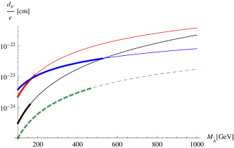
Figure 2: The maximal value of the muon EDM from flavor as a function of the average slepton mass based on Eqs. (8)–(12), and $y=1$. The three solid curves correspond to the current upper limit on ${\cal{B}}(\tau\to\mu\gamma)$, Eq. (2), and are obtained for $\delta^{L_{L}E}_{33}=10^{-3},10^{-4}$ and $10^{-2}$ (from top to bottom at $M_{\tilde{A}}=1000$ GeV). The dashed line refers to the hypothetical limit ${\cal{B}}(\tau\to\mu\gamma)$ $<2\cdot 10^{-9}$ for $\delta^{L_{L}E}_{33}=10^{-3}$. The thick curves have mass insertions $|\delta|<1$.

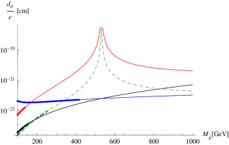
Figure 3: The same as in Fig. 2 but with the sign of $\delta^{L_{L}E}_{33}$ flipped, i.e., being negative.

We learn the following:

• Values of $d_{\mu}$ as large as ${\cal{O}}(10^{-22})\,\rm{ecm}$ are consistent with current FCNC constraints. For this to happen it requires ${\cal{O}}(1)$ intergenerational mixing. (The mass insertion approximation breaks down).

• The maximal allowed value of the muon EDM given by Eq. (12) grows with increasing $M_{\tilde{A}}$ and $y$.

• The muon EDM vanishes for vanishing stau LR-mixing $\delta^{L_{L}E}_{33}$ in our approximation. Large LR-mixing, however, suppresses $d_{\mu}$ because of the enhancement of the coefficient $\kappa$. For our parameters we find $\delta^{L_{L}E}_{33}\sim 10^{-(2-3)}$ to give the largest EDM, depending on the slepton mass.

• The sign of the stau chirality mixing matters: Negative values of $\delta^{L_{L}E}_{33}$ allow for larger EDMs by suppressing ${\cal{B}}(\tau\to\mu\gamma)$, see Eq. (11), at the price of increased tuning. This is illustrated in Fig. 3.

• Within the mass insertion approximation, $|\delta|\lesssim 1$, values of $d_{\mu}$ up to ${\cal{O}}(10^{-23})\,\rm{ecm}$ are possible if the sleptons have masses below a few hundred GeV, $\delta^{L_{L}E}_{33}\sim 10^{-(2-3)}$ and $y\lesssim{\cal{O}}(1)$.

• The maximal value for $d_{\mu}$ is proportional to the upper limit on ${\cal{B}}(\tau\to\mu\gamma)$. The anticipated future bound on ${\cal{B}}(\tau\to\mu\gamma)$ from super flavor factories of $2\cdot 10^{-9}$ Bona:2007qt has a significant impact on the maximal value of $d_{\mu}$.

II.3 Including Higgsinos

Since we neglect the mass of the muon, the higgsinos (and winos) do not contribute to $d_{\mu}$ to the order we are working, and Fig. 1 represents the leading contribution to the EDM. However, higgsino contributions have been found to be of importance in the calculation of ${\cal{B}}(\tau\to\mu\gamma)$ Feng:2001sq . More specifically, for a light $\mu$ term $\mu\sim M_{1},M_{2}$ the lightest neutralino has a substantial higgsino fraction and the photino-only approximation in the rare $\tau$ decays Eq. (10) receives large corrections. Consequently, the bounds on flavor violation change in the presence of the higgsinos, which then affects the maximal value of $d_{\mu}$ from flavor.

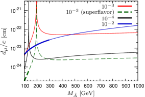
Figure 4: The maximal value of the muon EDM from flavor as a function of the average slepton mass based on Feng:2001sq for $\tan\beta=3$, $M_{1}=M_{\tilde{A}}$ and $\mu=2$ TeV. The three solid curves correspond to the current upper limit on ${\cal{B}}(\tau\to\mu\gamma)$, Eq. (2), and are obtained for $\delta^{L_{L}E}_{33}=10^{-2},10^{-3}$ and $10^{-4}$ (from top to bottom at $M_{\tilde{A}}=1000$ GeV). The dashed line refers to the hypothetical limit ${\cal{B}}(\tau\to\mu\gamma)$ $<2\cdot 10^{-9}$ for $\delta^{L_{L}E}_{33}=10^{-3}$. The thick curves have mass insertions $|\delta|<1$.

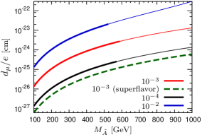
Figure 5: The same as in Fig. 4 but with $\mu=M_{\tilde{A}}$, hence lighter and more important higgsinos.

The higgsino contribution to the $\tau\to\mu\gamma$ amplitude involves directly the $\tau$ Yukawa coupling $y_{\tau}\propto\tan\beta$. Hence, keeping $\delta^{L_{L}E}_{33}$ fixed while enhancing $\tan\beta$, the higgsino loops get scaled up with respect to the bino ones and the maximal value of the muon EDM drops with respect to the analysis of the previous section. The same holds if the $A$-term dominates the stau LR-mixing, $\delta^{L_{L}E}_{33}\sim vA_{E,33}/\tan\beta$. If the $\mu$ term is large and dominates, $\delta^{L_{L}E}_{33}\sim-\mu m_{\tau}\tan\beta$, then all bino and higgsino contributions grow with $\tan\beta$. Since the EDM depends only linearly on $\delta^{L_{L}E}_{33}$, whereas ${\cal{B}}(\tau\to\mu\gamma)$ does quadratically, the maximal value of the EDM drops with increasing $\tan\beta$ also in this case. Therefore, large values of $d_{\mu}$ favor a low $\tan\beta$.

In Fig. 4 the maximal muon EDM as a function of the common slepton (smuon) mass is presented for the same values of $\delta^{L_{L}E}_{33}$ as in Fig. 2, however with the higgsino and wino contributions in ${\cal{B}}(\tau\to\mu\gamma)$ included. We use $\tan\beta=3,$ $\mu=2$ TeV, $M_{1}=M_{\tilde{A}}$ and $M_{2}=(g_{2}^{2}/g_{1}^{2})M_{1}$. As expected, a reasonably high value of $\mu$ suppresses the contribution from the higgsino loops, and, in general, the increase in ${\cal{B}}(\tau\to\mu\gamma)$ is small. Therefore, the photino analysis of Sec. II.2 gives a good approximation of the maximum value of the muon EDM. However, for low values of $\delta^{L_{L}E}_{33}$ the leading bino graphs in the $\tau\to\mu\gamma$ amplitude, which are proportional to $\delta^{L_{L}E}_{33}$, are suppressed, and external chirality flip graphs $\propto m_{\tau}$, which are usually sub-leading, become more important at the low slepton mass range. Therefore, a cancellation against the higgsino graphs occurs, which can be seen in Fig. 4 as a spike in the allowed maximal EDM curves. For larger values of $\delta^{L_{L}E}_{33}$ the cancellation does not happen, since the external flip contribution can not compete with the leading contributions.

In Fig. 5 we show the maximal muon EDM for an higgsino mass parameter $\mu$ which equals the slepton mass $M_{\tilde{A}}$. Consequently, the smaller $\mu$ term enhances the higgsino mediated loop contributions in ${\cal{B}}(\tau\to\mu\gamma)$ and the maximal EDM is not as large as in Figs. 2 or 4. With increasing slepton mass also $\mu$ increases, and the characteristics of Figs. 4 and 5 become alike.

Here, we assumed that $\delta_{23}^{\nu_{L}}$ is equal to $\delta_{23}^{L_{L}}$. Typically the sneutrino loop gives the largest single contribution to the branching ratio, unless the higgsinos are decoupled, in which case the bino loops dominate.

To summarize, the inclusion of higgsino contributions modifies the correlation between the maximal value of the muon EDM from flavor and ${\cal{B}}(\tau\to\mu\gamma)$ given in the previous section for low values of the $\mu$ term or when cancellations occur. Values of $d_{\mu}$ at order $10^{-22}\,\rm{ecm}$ are possible with current ${\cal{B}}(\tau\to\mu\gamma)$ constraints for order one flavor mixings. Values of order $10^{-23}\,\rm{ecm}$ can be reached within the mass insertion approximation, $|\delta|\lesssim 1$.

III Numerical analysis in the general MSSM

We study the muon EDM in the general MSSM neglecting CP phases unrelated to lepton flavor mixing. Formulae used are given in the appendix.

III.1 Input and Constraints on Susy Parameters

We generate sets of data points by randomly sampling susy parameters at the weak scale. We consider two scenarios, a ”light” and a ”heavy” one with their respective parameter ranges defined in Table 1.

	flavor diagonal	flavor off-diagonal
light	0 – 1 TeV	0 – 100 GeV
heavy	3 – 5 TeV	0– 3 TeV

Table 1: The sampling ranges for the flavor diagonal and off-diagonal mass parameters in the light and the heavy scenario.

As can be seen from Table 1, we use different ranges for the flavor diagonal and off-diagonal mass parameters. The former contain the gaugino masses $M_{1}$ and $M_{2}$, the $\mu$ term, its susy breaking companion, $B_{\mu}$, and the diagonal entries in the slepton soft terms $\sqrt{M^{2}_{L,ii}}$, $\sqrt{M^{2}_{E,ii}}$, $A_{E,ii}$. For simplicity we restrict our analysis to degenerate first and second generation masses $M^{2}_{L(E),11}=M^{2}_{L(E),22}$. Diagonal $A$-terms are assumed to follow the corresponding lepton Yukawa couplings $A_{E,ii}=A_{0}y_{i}$. Furthermore, we include slepton flavor mixing between the second and third generation only. The respective off-diagonal parameters are therefore $A_{E,23},A_{E,32},\sqrt{M^{2}_{L,23}}$ and $\sqrt{M^{2}_{E,23}}$. We allow for an order of magnitude suppression of the off-diagonal soft terms with respect to the diagonal entries in the light scenario, whereas in the heavy scenario we allow the off-diagonal terms to be of the same order of magnitude as the diagonal ones. In both scenarios $\tan\beta$ is sampled over the range 2 – 50.

For each generated point we check the scalar potential against unboundedness from below, and the existence of charge or color breaking minima Casas:1996de . These bounds constrain the off-diagonal soft contributions of the $A$-terms. The soft masses of the Higgs fields are solved for with the vacuum condition $\partial V/\partial\phi=0$. The resulting spectrum at each generated point is checked against experimental constraints from direct searches Amsler:2008zz . To generate a muon EDM we introduce random CP phases in all flavor off-diagonal soft terms between 0 and 2$\pi$. Since we assume here the $\mu-e$ and $\tau-e$ slepton mixing terms and all flavor blind CP violation to be zero, the experimental constraint from the electron EDM is automatically fulfilled. Contributions to $\mu\to e\gamma$ decays from sneutrino loops are also suppressed and neglected.

For each sample point, we calculate the contribution to the muon anomalous magnetic moment, $\Delta a_{\mu}$, the muon electric dipole moment $d_{\mu}$, and the branching ratio for the decay $\tau\to\mu\gamma$. $\Delta a_{\mu}$ is constrained to be less than $10^{-9}$ corresponding to roughly two sigma of the experimental and theoretical uncertainty DeRafael:2008iu . The bound on $\Delta a_{\mu}$ is always fulfilled in the heavy scenario.

III.2 Random Walk Analysis

The interplay between the muon EDM and the $\tau\to\mu\gamma$ branching ratio for our sampled points can be seen in Fig. 6. For both the light and heavy spectrum the value of the EDM for points satisfying ${\cal{B}}(\tau\to\mu\gamma)<10^{-8}$ is typically less than $10^{-24}$ ecm (squares and circles). This value is, however, not a hard upper bound on the muon EDM, because it stems from the stochastic nature of our parameter selection. Indeed, and as we will see, one can find parameters such that the constraint on the branching ratio is fulfilled and $d_{\mu}$ is large. The question then is how fine-tuned such points are.

$\log(d_{\mu}[\rm ecm])$
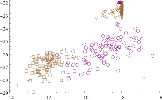
	$\log({\cal{B}}(\tau\to\mu\gamma))$

Figure 6: The distribution of the muon EDM $d_{\mu}$ vs. the branching ratio ${\cal{B}}(\tau\to\mu\gamma)$. Shown is the initial distribution in the light scenario (circles) and the heavy scenario (squares), as well as the distribution after the random walk process in the light (triangles up) and the heavy scenario (triangles down).

To obtain points with $d_{\mu}>(10^{-22}-10^{-24})$ ecm obeying the $\tau\to\mu\gamma$ constraint we use a random walk process. Starting from a point $p$ in parameter space, we randomly vary the parameters by a small amount, $p\to p^{\prime}=p+\delta p$, and check for all the constraints as well as for a larger value of the muon EDM. If $p^{\prime}$ passes the test, the procedure is repeated with $p^{\prime}$ as the new starting point. If we start out with a point $p$ that has ${\cal{B}}(\tau\to\mu\gamma)>10^{-8}$, we additionally require a decrease in the branching ratio before accepting $p^{\prime}$. The requirements on the branching ratio and the muon EDM thus drive a point into the desired direction. Unless we exceed a predetermined number of failed attempts, this procedure eventually yields a point with ${\cal{B}}(\tau\to\mu\gamma)<10^{-8}$ and a large value of $d_{\mu}$ as requested, after which the random walk is terminated.

In Fig. 6 we show the result of this random walk in the heavy and the light scenario. We see a tendency of points that start out with very low branching ratios to migrate to larger ones. This is expected, as the branching ratio has similar contributions as the EDM, which is being forced to increasing values. It should be noted that for the fixed number of iterations, we find that in the heavy scenario only about 2% of the original points achieved $d_{\mu}=10^{-22}$ ecm, whereas in the light scenario this fraction is 35%.

For each scenario we consider in the following two data sets, an inclusive one containing all the points that went through the random walk routine and an exclusive one containing only points that actually pass the EDM constraint $d_{\mu}\geq 10^{-22}$ ecm for the light scenario and $d_{\mu}\geq 0.5\cdot 10^{-22}$ ecm for the heavy scenario.

The random walk process affects the distribution of the parameters. E.g., in the light scenario there is a transition from a near flat distribution of $\tan\beta$ to one which is peaked at small values, see Fig. 7. The latter behavior is in agreement with the findings of Sec. II.3. In the next section we use this selection effect to construct a measure of fine-tuning.

# of points
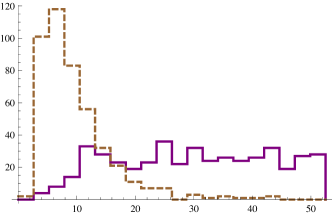
	$\tan\beta$

Figure 7: The distribution of $\tan\beta$ before (solid line) and after (dashed line) the random walk process in the light scenario (inclusive data set).

III.3 Measures of Fine-Tuning

In order to better understand the fine-tuning needed for achieving an experimentally interesting $d_{\mu}$ while respecting the experimental ${\cal{B}}(\tau\to\mu\gamma)$ constraint, we first note that the subamplitudes in $a^{L/R}_{23}$, see Eq. (51), corresponding to neutralino and chargino 1-loop Feynman diagrams, need to be small or cancel each other to great accuracy. We find that, however, there is usually only one subamplitude which contributes a dominant part of the branching ratio. When we increase the EDM via our random walk routine this disparity is lessened, but all individual subamplitudes remain small enough for there to be no need for large cancellations.

Similarly, Eq. (49) suggests that the imaginary part of $a^{R/L}_{22}$ needs to be as large as possible for a large EDM. Since in our framework there is only an imaginary part in the flavor off-diagonal 2-3 mixing, the subamplitudes in the initial data set exhibit a dominance of the real part over the imaginary part for all $a^{R/L}_{22}$’s. A priori, one would expect this relation to be reversed by the requirement to maximize $d_{\mu}$ but instead we end up with a sample, where the real and imaginary parts are within one order of magnitude of each other in the light scenario, and only slightly more dispersed in the heavy scenario. This is sufficient for generating a large EDM since the overall sizes of the subamplitudes have increased. We conclude that measures of fine-tuning which rely on looking at cancellations between different subamplitudes in magnitude or in imaginary part are not useful.

Another way of measuring fine-tuning is to look at the local structure of parameter space and see how sensitive observables are to variations of the parameters Barbieri:1987ed . We find that this measure of fine-tuning decreases for points when they go through our random walk process. This is expected since this method of measuring fine-tuning effectively looks at the slope in parameter space of a given observable, and in our case we drive these observables to their extremum values, i.e., to a region where the slope vanishes.

To discuss fine-tuning we instead consider the width of a parameter’s distribution and how the random walk process changes that width (see Fig. 7). From several such changes in the width we then construct a relative ”volume” of parameter space that is preferred by points that go through our random walk process. We do this by comparing the number of fixed and equi-distant bins in a parameter $X$ necessary to account for a given fraction $fr$ of points before, $N_{\mathrm{before}}$, and after, $N_{\mathrm{after}}$, the random walk process. This way, the bin number measures the width of a (normalized) distribution. The ratio, $r_{X}\equiv(N_{\mathrm{after}}/N_{\mathrm{before}})$, gives us a measure of how much the range of the parameter $X$ has shrunk (peaked), $r_{X}<1$, or expanded (flattened), $r_{X}>1$. Smaller (larger) volume fractions $r_{X}$ then correspond to larger (smaller) tuning. For the $\tan\beta$-distributions shown in Fig. 7 we obtain $r_{\tan\beta}=0.25$ (for $fr=0.8$).

We consider the tuning of several parameters, specifically, the CP phases of the four flavor off-diagonal soft terms, masses and $\tan\beta$.

Before proceeding, we note a couple of caveats. First, while random walking the range of some parameters can expand beyond the range to which we have initially constrained them, e.g., the diagonal soft terms in the heavy scenario are sampled between 3 and 5 TeV, and the random walk process moves and spreads this range out. Since this is an artificial diffusion effect (and we can effectively choose $r_{X}$ to be whatever we want by adjusting the initial sampling range) we exclude such parameters directly from the measure of fine-tuning. Secondly, even though a parameters distribution remains unchanged, it may become correlated with another parameter. An example for this are the complex phases of the off-diagonal soft mass terms. Let $2\phi_{X_{23}}=\arg(M^{2}_{X,23})$ for $X=L,E$. While we find for each $\phi_{L_{23}}$ and $\phi_{E_{23}}$ separately the ratio $r\simeq 1$, their difference $\Delta\phi=\phi_{L_{23}}-\phi_{E_{23}}$ has $r_{\Delta\phi}\simeq 0.47$ with sharp peaks around $\pi/4$ and $3\pi/4$ (heavy scenario), as can be seen in Fig. 8. This correlation can be understood from Eq. 9, with ${\rm Im}(\delta^{L_{L}}_{23}\delta^{L_{L}E}_{33}\delta^{E*}_{23})$ maximized.

# of points
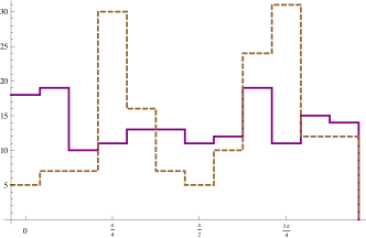
	$\phi_{L_{23}}-\phi_{E_{23}}$

Figure 8: The distribution of $\phi_{L_{23}}-\phi_{E_{23}}$ before (solid line) and after (dashed line) the random walk process in the heavy scenario (exclusive data set).

We investigate the phase differences of $M^{2}_{X,23}$, $X=L,E$ and $A_{E,23},A_{E,32}$, and assign the product of the individual volume changes $r_{\Delta\phi_{i}}$ as

$$d_{\phi}=\prod_{i}r_{\Delta\phi_{i}}.$$ (13)

Furthermore, we consider various ratios of mass parameters. We examine the following ratios containing off-diagonal entries:

$$\frac{|M^{2}_{L,23}|}{M^{2}_{L,33}},\frac{|M^{2}_{E,23}|}{M^{2}_{E,33}},\frac{|A_{E,23}|}{A_{0}},\frac{|A_{E,32}|}{A_{0}}.$$ (14)

The product of their individual volume fractions is denoted by $d_{od}$. We look at some general ratios of parameters in the slepton sector and the mass parameters $M_{1}$, $M_{2}$, $\mu$:

$$\frac{\sqrt{M^{2}_{L,22}-M^{2}_{L,33}}}{\frac{1}{2}(\sqrt{M^{2}_{L,22}}+\sqrt{M^{2}_{L,33}})},\frac{\sqrt{M^{2}_{E,22}-M^{2}_{E,33}}}{\frac{1}{2}(\sqrt{M^{2}_{E,22}}+\sqrt{M^{2}_{E,33}})},$$

$$\frac{\sqrt[4]{M^{2}_{L,33}M^{2}_{E,33}}}{A_{0}},\frac{\sqrt[4]{M^{2}_{L,33}M^{2}_{E,33}}}{M_{1}},\frac{\sqrt{M_{1}M_{2}}}{\mu},\frac{M_{1}}{M_{2}}.$$ (15)

The product of their individual volume fractions is denoted by $d_{G}$. We then define a total change of volume of parameter space, $d_{V}$, as

$$d_{V}=d_{\phi}\cdot d_{od}\cdot d_{G}\cdot r_{\tan\beta}.$$ (16)

One would expect that the volume changes $d_{X}$ depend on the value of the fraction of points, $fr$. In Fig. 9 we show this dependence for $d_{V}$. As can be seen, $d_{V}$ is very stable over a large range of $fr$. The unstable behavior for values of $fr\gtrsim 0.8$ is due to the way statistical outliers affect our analysis. A more sophisticated approach to measuring the width of parameter distributions by fitting, e.g., Gaussian curves could improve the stability. We also verify that the values of the $r_{X}$’s (and consequently $d_{X}$’s) remain stable under variations of spurious quantities such as changes in data binning.

$\log(d_{V})$
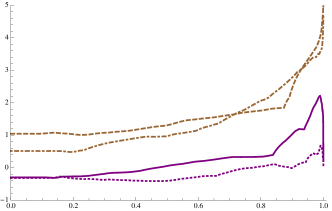
	$fr$

Figure 9: The parameter space volume fraction $d_{V}$ Eq. (16) as a function of $fr$ in the light inclusive (solid line), light exclusive (dotted line), heavy inclusive (dashed line), and heavy exclusive (dash-dotted line) scenario.

III.4 Discussion

The various volume fractions for the two scenarios and data sets are shown in Table 2 for $fr=0.8$. Comparing the different entries, we get an idea about fine-tuning caused by the random walk process.

Notably, the effect of the CP phases becoming correlated (as shown in Fig. 8) emerges in the exclusive heavy scenario only. Also we see that a tuning of $\tan\beta$ occurs in the light scenario only (see Fig. 7).

	Inclusive		Exclusive
	Light	Heavy	Light	Heavy
$r_{\tan\beta}$	0.25	0.96	0.16	0.95
$d_{od}$	1.3	0.88	2.9	10
$d_{\phi}$	0.98	0.96	0.98	0.49
$d_{G}$	1.8	69	0.39	33
$d_{V}$	2.2	59	1.1	170

Table 2: The volume fractions of parameter space after the random walk for $fr=0.8$ for the light and the heavy scenario. Smaller numbers correspond to larger tuning.

The ratios of the off-diagonal to diagonal mass elements which we have collected into $d_{od}$, have values close to unity in the inclusive set but spread out, by up to an order of magnitude in the case of heavy scenario, when we look at the exclusive set. This means that the more fine-tuned the points get, the wider the range of acceptable mass ratios is. These ratios enter the loop contributions of the branching ratio and EDM and their increase in size, which leads to the spreading out of the distribution, is in line with the observations from the beginning of Sec. III.3.

Finally, we see that for the set of flavor diagonal mass ratios in $d_{G}$, there is a fine-tuning effect in the light scenario that emerges for the exclusive set, whereas in the heavy scenario there is instead again a spreading out.

It is apparent that the ranges for the mass ratios are more constrained in the light scenario. In the heavy scenario, the individual loop contributions (which partly depend on these mass ratios) start out much smaller than in the light scenario and thus there is more “room” to spread out. The phases $\phi_{L_{23}}$ and $\phi_{E_{23}}$ becoming correlated is also a sign of insufficient size of the loop contributions.

It needs to be emphasized that the change in parameter space volume is a relative measure of the amount of fine-tuning and useful for comparisons between different data sets. It is not an absolute measure of the ease of fine-tuning. Even comparing different rows in Table 2 is not trivial, e.g., fine-tuning the phases can have a greater or lesser effect on the EDM than fine-tuning the mass ratios.

We find that both heavy and light scenarios appear to be not particularly tuned to give a large value of the muon EDM while respecting existing constraints. While most of the volume fractions $d_{X}$ in the light scenario are smaller than in the heavy one, from looking at Fig. 6 and noting that a large percentage ($\sim$98%) of points in the heavy scenario can not be tuned to high enough values of $d_{\mu}$, we conclude that the heavy scenario is quantitatively harder to fine-tune.

IV A Flavored EDM in Hybrid models

After analyzing the muon EDM within the general MSSM, we now consider the situation in an explicit model with a hybrid mechanism of susy breaking, gauge-gravity mediation. These models have recently received attention because they provide insights into the nature of flavor breaking due to the appearance of flavor structures beyond the Yukawa couplings Feng:2007ke ; Hiller:2008sv ; Nomura:2007ap ; Hiller:2010dv . Viable gauge-gravity models have the dominant source of susy breaking from gauge mediation, which is flavor-blind at the scale of mediation. Additional contributions arise from Planck-scale gravity, which generically affect flavor physics. We assume here that the latter is controlled by Froggatt-Nielsen (FN) symmetries Froggatt:1978nt , generating also the Yukawa matrices.

At the scale of gauge mediation, $m_{M}$, we parametrize the soft terms of the sleptons as Feng:2007ke

$$M_{L}^{2}(m_{M}) = \tilde{m}_{L}^{2}(\mathbf{1}+x_{2}X_{L}),$$

$$M_{E}^{2}(m_{M}) = \tilde{m}_{E}^{2}(\mathbf{1}+x_{1}X_{R}).$$ (17)

The new flavor structure from gravity with respect to gauge mediation is encoded in the hermitean matrices $X_{L,R}$, following from the charge assignments of the FN-symmetry. The factors $x_{1}$ and $x_{2}$ implicitly defined by Eq. (17) quantify the relative size of the gravity versus the gauge contribution to the $SU(2)$ singlet and doublet soft masses, respectively. In this way, the $x_{i}$ are measures of the separation between the messenger and the Planck scale, $m_{\rm Pl}$. In minimal gauge mediation with $N_{M}$ messengers (see, e.g., Martin:1997ns ),

$$x_{i}\sim\left(\frac{m_{M}}{m_{\rm Pl}}\right)^{2}\left(\frac{4\pi}{\alpha_{i}(m_{M})}\right)^{2}\frac{c_{i}}{N_{M}},\,c_{1}=\frac{5}{6},c_{2}=\frac{2}{3},$$ (18)

where we assumed that the $F$-terms from $m_{\rm Pl}$ couple also to gauge mediation. The ratio $x_{1}/x_{2}$ as in Eq. (18) is of order one, and increases for lower values of the messenger scale, see Fig. 10.

Figure 10: The ratio $x_{1}/x_{2}$ in minimal gauge mediation Eq. (18) as a function of the messenger scale.

In Section IV.1 we give formulae for the flavor violating low energy parameters in gauge-gravity models. A flavor model with explicit FN charges is studied in Section IV.2. We investigate the impact of trilinear $A$-terms in Section IV.3.

IV.1 Hybrid Gauge-Gravity

Starting from the soft slepton masses at the scale $m_{M}$ of the form given in Eq. (17) and solving the MSSM renormalization group (RG) equations Martin:1993zk , the soft slepton masses at the weak scale can be written in the following approximate form:

$$M^{2}_{L}(m_{Z}) \sim \tilde{m}^{2}_{L}(r_{2}{\bf 1}+c_{L}Y_{e}Y_{e}^{\dagger}+x_{2}X_{L}),$$

$$M^{2}_{E}(m_{Z}) \sim \tilde{m}^{2}_{E}(r_{1}{\bf 1}+c_{E}Y_{e}^{\dagger}Y_{e}+x_{1}X_{R}).$$ (19)

In the spirit of the FN flavor models, Eq. (19) and the following estimations are only accurate up to numbers of order one, which we indicate by ”$\sim$”. The running of the gravity-induced terms is such an order one effect. The coefficients $c_{L},c_{E}$ are negative, obey $|c_{L}|<|c_{E}|$ and are of the order $\sim 1/(16\pi^{2})\ln(m_{M}/m_{Z})$, which are at most of order one for $m_{M}$ near the GUT scale.

The $r_{i}$ coefficients include the leading RG correction to the flavor diagonal elements. Neglecting contributions from the sub-leading gauge couplings, one obtains an analytical expression for $r_{i}$ at one-loop order (see, e.g., Martin:1997ns ):

$$r_{i}=1+\frac{1}{c_{i}\pi}\left(\int_{\ln(m_{Z})}^{\ln(m_{M})}dt\frac{\alpha_{i}^{3}(t)}{\alpha_{i}^{2}(m_{M})}\right)\frac{M_{i}^{2}(m_{M})}{\tilde{m}_{i}^{2}(m_{M})}.$$ (20)

Here, $M_{i}$ denotes the respective gaugino mass and $\tilde{m}_{i}^{2}$ equals $\tilde{m}_{L}^{2}$ for $i=2$ and $\tilde{m}_{E}^{2}$ for $i=1$. In messenger models of gauge mediation, the ratio $M_{i}^{2}/\tilde{m}_{i}^{2}$ is determined by a simple formula at the scale of mediation including only the leading gauge contributions:

$$\frac{M_{i}^{2}(m_{M})}{\tilde{m}^{2}_{i}(m_{M})}=c_{i}N_{M}.$$ (21)

The RG parameters $r_{i}$ from Eqs. (20) and (21) obey $r_{2}>r_{1}>1$ and are of order one for not too many messengers. Since $r_{i}>1$, the RG effect strengthens the flavor blind entries hence reduces the flavor violation. The properties of the $r_{i}$ can be different in general gauge mediation Meade:2008wd which does not exclude negative soft sfermion masses-squared at the mediation scale.

In the basis where the leptons are mass eigenstates and the neutralino interactions are diagonal in generation space we obtain:

$$\widetilde{M}^{2}_{L_{L}}(m_{Z}) \sim \tilde{m}^{2}_{L}(r_{2}{\bf 1}+c_{L}D_{e}^{2}+x_{2}V_{L_{L}}X_{L}V_{L_{L}}^{\dagger}),$$

$$\widetilde{M}^{2}_{\nu_{L}}(m_{Z}) \sim \tilde{m}^{2}_{L}(r_{2}{\bf 1}+c_{L}U^{\dagger}D_{e}^{2}U+x_{2}V_{\nu_{L}}X_{L}V_{\nu_{L}}^{\dagger}),$$

$$\widetilde{M}^{2}_{E}(m_{Z}) \sim \tilde{m}^{2}_{E}(r_{1}{\bf 1}+c_{E}D_{e}^{2}+x_{1}V_{E}X_{R}V_{E}^{\dagger}),$$ (22)

where $U=V_{L_{L}}V^{\dagger}_{\nu_{L}}$ denotes the Maki-Nakagawa-Sakata (MNS) matrix and $D_{e}={\rm diag}(y_{e},y_{\mu},y_{\tau})=V_{L_{L}}Y_{e}V_{E}^{\dagger}$. Note that the parametrization Eq. (22) holds beyond minimal gauge mediation with perturbative messengers.

The mass insertions of the charged sleptons are then given as ($i\neq j$)

$$\delta^{L_{L}}_{ij}\sim\frac{x_{2}}{r_{2}}(V_{L_{L}}X_{L}V_{L_{L}}^{\dagger})_{ij},~{}~{}\delta^{E}_{ij}\sim\frac{x_{1}}{r_{1}}(V_{E}X_{R}V_{E}^{\dagger})_{ij}.$$ (23)

Here, we neglected contributions in the denominators from the tau-yukawa of the order $y_{\tau}^{2}\sim 10^{-4}\tan^{2}\beta$ with respect to the $r_{i}$ for mixings involving the third generation. The sneutrino mass insertions, which matter for the rare decays only to the order we are working, $m_{\mu}=0$, are given as ($i\neq j$)

$$\delta^{\nu_{L}}_{ij}\sim\frac{1}{r_{2}}\left(c_{L}y_{\tau}^{2}U^{*}_{3i}U_{3j}+x_{2}(V_{\nu_{L}}X_{L}V_{\nu_{L}}^{\dagger})_{ij}\right),$$ (24)

receiving two independent competing contributions. Note that the second term in Eq. (24) equals $U^{*}_{ki}\delta^{L_{L}}_{kl}U_{lj}$. Since its sign/phase is not fixed by the FN symmetry, there can be cancellations in $\delta^{\nu_{L}}_{ij}$.

IV.2 A Flavor Model and Phenomenology

Following Ref. Feng:2007ke we entertain a $U(1)\times U(1)$ FN symmetry with a single symmetry breaking parameter $\lambda$ of the order $0.1-0.2$. Specifically, we use the following horizontal charges

$$L_{1}(2,0),L_{2}(0,2),L_{3}(0,2),$$

$$\bar{E}_{1}(2,1),\bar{E}_{2}(2,-1),\bar{E}_{3}(0,-1),$$ (25)

which result in a large 2-3 mixing. The lepton mixing angles are obtained as

$$(V_{L_{L}})_{12} \sim \lambda^{8},(V_{L_{L}})_{13}\sim\lambda^{8},(V_{L_{L}})_{23}\sim 1,$$

$$(V_{E})_{12} \sim \lambda^{2},(V_{E})_{13}\sim\lambda^{4},(V_{E})_{23}\sim\lambda^{2},$$

$$(V_{\nu_{L}})_{ij} \sim 1,$$ (26)

leading to $U_{ij}\sim{\cal{O}}(1)$. The current level of suppression of the 1-3 lepton mixing is considered accidental.

The slepton soft terms have the flavor structure

$$(X_{L})_{12} \sim \lambda^{4},(X_{L})_{13}\sim\lambda^{4},(X_{L})_{23}\sim 1,$$

$$(X_{R})_{12} \sim \lambda^{2},(X_{R})_{13}\sim\lambda^{4},(X_{R})_{23}\sim\lambda^{2},$$ (27)

with the diagonal ones $(X_{L,R})_{ii}\sim 1$. Inserting the factors $X_{L,R}$ and the mixing angles into Eq. (22) the flavor changing mass insertions are obtained as

$$\delta^{L_{L}}_{12} \sim \frac{x_{2}}{r_{2}}\lambda^{4},~{}~{}\delta^{E}_{12}\sim\frac{x_{1}}{r_{1}}\lambda^{2},~{}~{}\delta^{\nu_{L}}_{12}\sim\frac{1}{r_{2}}(c_{L}y_{\tau}^{2}+x_{2}),$$

$$\delta^{L_{L}}_{13} \sim \frac{x_{2}}{r_{2}}\lambda^{4},~{}~{}\delta^{E}_{13}\sim\frac{x_{1}}{r_{1}}\lambda^{4},~{}~{}\delta^{\nu_{L}}_{13}\sim\frac{1}{r_{2}}(c_{L}y_{\tau}^{2}+x_{2}),$$

$$\delta^{L_{L}}_{23} \sim \frac{x_{2}}{r_{2}},~{}~{}\delta^{E}_{23}\sim\frac{x_{1}}{r_{1}}\lambda^{2},~{}~{}\delta^{\nu_{L}}_{23}\sim\frac{1}{r_{2}}(c_{L}y_{\tau}^{2}+x_{2}).$$ (28)

The relevant coupling for the muon EDM in this model is hence given as $\delta^{L_{L}}_{23}\delta^{E*}_{23}\sim x_{1}x_{2}/(r_{1}r_{2})\lambda^{2}\lesssim 0.04$.

We illustrate the correlation between the rare decays and the muon EDM for near maximal mass insertions $\delta^{L_{L}}_{23}=i0.8$ and $\delta^{E}_{23}=0.05$ and various higgsino parameters and stau LR-mixings in Fig. 11.

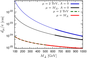
Figure 11: The muon EDM in the flavor model Eq. (IV.2) with different $\mu$ terms and stau LR-mixings. Fad lines are consistent with the ${\cal{B}}(\tau\to\mu\gamma)$ bound Eq. (2). In all curves $\tan\beta=3$ and $M_{\tilde{A}}=M_{1}$. The lower two, overlapping curves use $\delta^{L_{L}E}_{33}=10^{-3}$.

Fad lines are in agreement with the current ${\cal{B}}(\tau\to\mu\gamma)$ bound. The two upper curves have a negatively valued stau LR-mixing induced by the $\mu$ term. The lower two, overlapping curves use $\delta^{L_{L}E}_{33}=10^{-3}$. Here, again, a larger $\mu$ term (dashed curve) gives heavier higgsinos and allows for a larger $d_{\mu}$ by relaxing the constraint from the $\tau\to\mu\gamma$ decays.

The constraint from the FCNC can be avoided in the hybrid models by suppressing flavor violation by increasing the separation between the Planck and the messenger scale. The exact value of the upper bound on $x_{i}/r_{i}$ in the model Eq. (IV.2) depends on the susy spectrum and composition and is rather weak due to the strong suppression of 1-2 mixing, which passes the $\mu\to e\gamma$ constraint. For example, for the parameters along the fad lines in Fig. 11 holds $x_{i}/r_{i}\lesssim{\cal{O}}(1)$.

We obtain in the flavor model Eq. (IV.2) for the maximal value of the muon EDM

$$\frac{d_{\mu}}{e}\lesssim 5\cdot 10^{-24}{\rm cm},$$ (29)

in agreement with existing data, specifically the FCNC constraints Eq. (2). The other FN models of Ref. Feng:2007ke have smaller values of $\delta^{L_{L}}_{23}\delta^{E*}_{23}$, hence yield smaller values of $d_{\mu}$, either due to a smaller 2-3 mixing, or by a stronger constraint on $x_{i}/r_{i}$ effective for less suppressed 1-2 mixing.

We conclude that an observation of the muon EDM at the level of order $10^{-(23-24)}\,{\rm ecm}$ would imply the following in the context of gauge-gravity models with a FN symmetry:

• The flavor structure needs to be very specific, i.e. not every FN symmetry correctly reproducing the SM lepton masses and mixings works.

• CP is broken together with flavor, and the CP phases are unsuppressed.

• The susy spectrum is not too heavy, of the order of a few 100 GeV, and $y\lesssim 1$.

• The messenger scale needs to be very high, not far from $m_{M}\sim\alpha/(4\pi)m_{\rm Pl}$.

Note that analogous studies in the quark sector have found that FCNC data constrain the messenger scale in typical FN models to be about three orders of magnitude below $m_{\rm Pl}$ Hiller:2008sv .

IV.3 Including $A$-terms

The gauge mediated contribution to the trilinear $A$-terms is of higher order and usually set to zero $A_{E}(m_{M})=0$. This has also been employed implicitly in the previous section. While the MSSM RG equations do induce finite $A$-terms at the weak scale, however, such terms do not introduce CP or flavor violation beyond the Yukawa matrices, and do not matter for flavor phenomenology.

However, in our hybrid set-up, there can be a finite contribution from gravity to the $A$-terms Hiller:2010dv :

$$A_{E}(m_{M})\sim\sqrt{\tilde{m}^{2}x}Y_{e},$$ (30)

where we used that the gravity-induced $A$-terms receive the same parametric suppressions from the flavor symmetry breaking as the corresponding Yukawa matrices. Here, $\tilde{m}^{2},x$ are of the order of $\tilde{m}_{E}^{2}$ and $\tilde{m}_{L}^{2}$, $x_{1}$ and $x_{2}$, respectively.

We then evolve according to the MSSM RG equations. The result can be recast in the following approximate form

$$A_{E}(m_{Z})\sim Y_{e}(a_{E}+\sqrt{\tilde{m}^{2}x}+b_{E}Y_{e}^{\dagger}Y_{e}).$$ (31)

The dominant contribution to $a_{E}$ and $b_{E}$ stems from the gaugino masses, which drives them to magnitudes of electroweak size for large enough $m_{M}$. Note that $a_{E}<0$ and $b_{E}>0$. Unless $\tan\beta$ is very large, the double Yukawa-suppression makes the $b_{E}$ term negligible. As indicated in Eq. (31), the gravity contribution evolves with a coefficient of order one.

In the basis with lepton mass eigenstates and diagonal neutralino couplings we obtain:

$$\tilde{A}_{E} = V_{L_{L}}A_{E}V_{E}^{\dagger}$$ (32)

$$\sim D_{e}(a_{E}+\sqrt{\tilde{m}^{2}x}+b_{E}D_{e}^{2}).$$

Under the RG evolution the $A$-terms mix onto the soft masses squared and induce also corrections to the soft masses in Eq. (22). Due to the Yukawa texture, this results effectively into a correction of the order $x$ of the $c_{L,E}$ coefficients, and will be absorbed therein for the purpose of this work.

The strongest bound on the hybrid model including $A$-terms Eq. (30) is from the electron EDM, stemming from $\delta^{L_{L}E}_{11}$ and its imaginary part. An approximate expression for $d_{e}$ reads as, see, Eq. (8) for the corresponding formula for $d_{\mu}$,

$$\frac{d_{e}}{e} = \frac{\alpha}{2\pi}\frac{M_{i}}{M_{\tilde{A}}^{2}}G_{1}(y){\rm Im}(\delta^{L_{L}E}_{11}),$$ (33)

$$\lesssim 2.6\cdot 10^{-26}{\rm cm}\left(\frac{200\mbox{GeV}}{M_{\tilde{A}}}\right)^{2}\sqrt{\frac{x}{r}},$$

where we assumed $y=1$ in the second line. Here, CP violation is induced by the gravity-mediated $A$-terms, Eq. (30), which are fixed by the FN symmetry up to order one, in general complex numbers, only. One obtains from Eqs. (I) and (33):

$$x/r\lesssim 5\cdot 10^{-3}.$$ (34)

This bound implies a separation between the Planck scale and the messenger scale of about up to four orders of magnitude, see Fig. 12. Information on the hadronic sector, that is, the neutron EDM in a similar set-up with Yukawa-like $A$-terms and a viable quark FN symmetry gives somewhat milder constraints Hiller:2010dv .

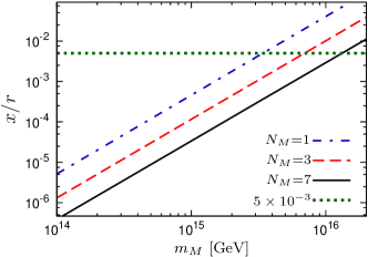
Figure 12: The ratio $x/r$ in minimal gauge mediation Eq. (18) as a function of the messenger scale. The curves correspond to $N_{M}=1,3$ and 7 (from top to bottom). The horizontal line denotes the constraint from the electron EDM, Eq. (34).

The bound Eq. (34) excludes a muon EDM from flavor since the mass insertions are subsequently suppressed as

$$\delta^{L_{L}}_{23}\delta^{E*}_{23}\sim\lambda^{k}(x/r)^{2}\lesssim\lambda^{k}10^{-5}\leq 10^{-5},$$ (35)

where $k$ denotes the non-negative integer power from the FN charges of a given model.

So far, we assumed the CP phase $\phi$ of $A_{E,11}$ to be fully unsuppressed. The bound Eq. (34) weakens by a factor $1/\sin^{2}\phi$ if $\phi$ is not maximal. However, for $k=2$ as in the model from the previous section, even with a phase suppression as low as $\sin\phi$ at the percent level, the prediction for $d_{\mu}$ is as in the linear mass scaling case, Eq. (3).

V Summary

Observing a large muon EDM $d_{\mu}\gtrsim{\cal{O}}(10^{-24})\,{\rm ecm}$ requires CP violation from flavor violation and favors a light mass spectrum. The heavier the spectrum and the larger the higgsino admixture, the larger is the requisite tuning to avoid the most relevant flavor constraint, ${\cal{B}}(\tau\to\mu\gamma)$.

In the context of hybrid gauge-gravity models a measurement of such large values of the muon EDM would point towards a specific Planck scale flavor structure and a very large messenger scale not far from $\sim\alpha/(4\pi)m_{\rm Pl}$. In the presence of Yukawa-textured $A$-terms at the level of Eq. (30) with CP phases, however, the muon EDM is limited by the electron EDM data to follow the linear mass scaling constraint Eq. (3), which is below the current experimental sensitivity.

We conclude that the muon EDM is informative on various aspects of the underlying fundamental physics.

Appendix A The relevant MSSM parameters

The notation follows closely Ref. Bartl:2003ju ; Rosiek:1995kg .

A.1 Mixing matrices

The slepton mass-squared matrices Eqs. (4) and (6) are diagonalized by the matrices $R^{\tilde{l}/\tilde{\nu}}$:

$$R^{\tilde{l}/\tilde{\nu}}M^{2}_{\tilde{l}/\tilde{\nu}}(R^{\tilde{l}/\tilde{\nu}})^{-1} = \mathrm{diag}(M^{2}_{\tilde{l}/\tilde{\nu}}).$$ (36)

The neutralino and chargino mass matrices are as usual

$$M_{\chi_{0}} = \left(\begin{array}[]{cccc}M_{1}&0&-{g^{\prime}v_{1}\over\sqrt{2}}&{g^{\prime}v_{2}\over\sqrt{2}}\\ 0&M_{2}&{gv_{1}\over\sqrt{2}}&-{gv_{2}\over\sqrt{2}}\\ -{g^{\prime}v_{1}\over\sqrt{2}}&{gv_{1}\over\sqrt{2}}&0&-\mu\\ {g^{\prime}v_{2}\over\sqrt{2}}&-{gv_{2}\over\sqrt{2}}&-\mu&0\end{array}\right),$$ (41)

$$M_{\chi_{\pm}} = \left(\begin{array}[]{cc}M_{2}&gv_{2}\\ gv_{1}&\mu\end{array}\right),$$ (44)

where $M_{1}$ and $M_{2}$ are the $U(1)$ and $SU(2)$ gaugino soft masses, respectively, and $g^{\prime}=e/\cos\theta_{W}=\sqrt{3/5}g_{1}$, $g=e/\sin\theta_{W}=g_{2}$. The neutralino and chargino mass matrices are diagonalized by matrices $N$ and $U,V$ as follows:

$$U^{\ast}M_{\chi^{\pm}}V^{-1} = \mathrm{diag}(M_{\chi^{\pm}}),$$

$$N^{\ast}M_{\chi^{0}}N^{-1} = \mathrm{diag}(M_{\chi^{0}}).$$ (45)

A.2 Leptonic observables

The relevant Lagrangian involving sleptons, neutralinos and charginos is as follows:

$$\mathcal{L} = \bar{l}_{i}(n_{ijk}^{L}L+n_{ijk}^{R}R)\chi_{j}^{0}\tilde{l}_{k}^{\vphantom{\ast}}$$ (46)

$$+\bar{l}_{i}(c_{ijk}^{L}L+c_{ijk}^{R}R)\chi_{j}^{-}\tilde{\nu}_{k}^{\vphantom{\ast}}+\mathrm{h.c.},$$

where

$$c_{ijk}^{R} \equiv -gV_{j1}^{\vphantom{\ast}}R_{ki}^{\tilde{\nu}\ast},$$

$$c_{ijk}^{L} \equiv y_{i}^{\vphantom{\ast}}U_{j2}^{\ast}R_{ki}^{\tilde{\nu}\ast},$$

$$n_{ijk}^{L} \equiv -g^{\prime}\sqrt{2}N_{j1}^{\ast}R_{k,i+3}^{\tilde{l}\ast}-y_{i}^{\vphantom{\ast}}N_{j3}^{\ast}R_{ki}^{\tilde{l}\ast},$$ (47)

$$n_{ijk}^{R} \equiv \left(g^{\prime}N_{j1}^{\vphantom{\ast}}+gN_{j2}^{\vphantom{\ast}}\right)R_{ki}^{\tilde{l}\ast}/\sqrt{2}-y_{i}^{\ast}N_{j3}^{\vphantom{\ast}}R_{k,i+3}^{\tilde{l}\ast}.$$

The susy contributions to the radiative lepton decay width, the lepton EDM, and the magnetic moment can be written at one-loop as Bartl:2003ju

$$\Gamma(l_{j}\to l_{i}\gamma) = {\alpha m_{l,j}\over 16}(|a_{ij}^{L}|^{2}+|a_{ij}^{R}|^{2}),$$ (48)

$$d_{i} = {e\over 4m_{l,i}}\mathrm{Im}(-a_{ii}^{L}+a_{ii}^{R}),$$ (49)

$$\Delta a_{i} = {1\over 2}\mathrm{Re}(a_{ii}^{L}+a_{ii}^{R}),$$ (50)

where terms of order $\mathcal{O}(m_{l_{i}}/m_{l_{j}})$ have been dropped. The coefficients $a_{ij}^{L,R}$ are given as

$$a_{ij}^{L} = {1\over 16\pi^{2}}\sum_{k=1}^{4}\sum_{r=1}^{6}\left(\left(n_{ikr}^{L}n_{jkr}^{L\ast}{m_{l,j}^{2}\over m_{\tilde{\chi}_{k}^{0}}^{2}}+n_{ikr}^{R}n_{jkr}^{R\ast}{m_{l,i}^{2}\over m_{\tilde{\chi}_{k}^{0}}^{2}}\right)\right.$$

$$\left.\times F_{1}\left({m_{\tilde{l}_{r}}^{2}\over m_{\tilde{\chi}_{k}^{0}}^{2}}\right)+n_{ikr}^{L}n_{jkr}^{R\ast}{m_{l,j}\over m_{\tilde{\chi}_{k}^{0}}}F_{3}\left({m_{\tilde{l}_{r}}^{2}\over m_{\tilde{\chi}_{k}^{0}}^{2}}\right)\right)$$

$$+ {1\over 16\pi^{2}}\sum_{k=1}^{2}\sum_{r=1}^{3}\left(\left(c_{ikr}^{L}c_{jkr}^{L\ast}{m_{l,j}^{2}\over m_{\tilde{\chi}_{k}^{+}}^{2}}+c_{ikr}^{R}c_{jkr}^{R\ast}{m_{l,i}^{2}\over m_{\tilde{\chi}_{k}^{+}}^{2}}\right)\right.$$

$$\left.\times F_{2}\left({m_{\tilde{\nu}_{r}}^{2}\over m_{\tilde{\chi}_{k}^{+}}^{2}}\right)+c_{ikr}^{L}c_{jkr}^{R\ast}{m_{l,j}\over m_{\tilde{\chi}_{k}^{+}}}F_{4}\left({m_{\tilde{\nu}_{r}}^{2}\over m_{\tilde{\chi}_{k}^{+}}^{2}}\right)\right),$$

$$a_{ij}^{R} = a_{ij}^{L}(L\leftrightarrow R),$$ (51)

where

$$F_{1}(x) = -{2+3x-6x^{2}+x^{3}+6x\mathrm{log}x\over 6(1-x)^{4}},$$ (52)

$$F_{2}(x) = {1-6x+3x^{2}+2x^{3}-6x^{2}\mathrm{log}x\over 6(1-x)^{4}},$$ (53)

$$F_{3}(x) = -{1-x^{2}+2x\mathrm{log}x\over(1-x)^{3}},$$ (54)

$$F_{4}(x) = {1-4x+3x^{2}-2x^{2}\mathrm{log}x\over(1-x)^{3}}.$$ (55)

The functions $G_{1,3}$ relevant for the calculation in the mass insertion approximation are obtained from Eqs. (52) and (54) as $G_{3}(1/x)=(x^{2}/2)\cdot\partial F_{1}/\partial x$ and $G_{1}(1/x)=(x^{2}/2)\cdot\partial F_{3}/\partial x$.

References

- (1) M. Pospelov and A. Ritz, Annals Phys. 318, 119 (2005) [arXiv:hep-ph/0504231].
- (2) M. E. Pospelov and I. B. Khriplovich, Sov. J. Nucl. Phys. 53, 638 (1991) [Yad. Fiz. 53, 1030 (1991)].
- (3) C. Amsler et al. [Particle Data Group], Phys. Lett. B 667, 1 (2008).
- (4) G. W. Bennett et al. [Muon (g-2) Collaboration], Phys. Rev. D 80, 052008 (2009) [arXiv:0811.1207 [hep-ex]].
- (5) B. Aubert et al. [BABAR Collaboration], Phys. Rev. Lett. 104, 021802 (2010), arXiv:0908.2381 [hep-ex].
- (6) G. Signorelli, J. Phys. G 29, 2027 (2003).
- (7) M. Bona et al., arXiv:0709.0451 [hep-ex].
- (8) A. Adelmann et al., arXiv:hep-ex/0606034v2; A. Adelmann, K. Kirch, C. J. G. Onderwater and T. Schietinger, J. Phys. G 37, 085001 (2010).
- (9) J. L. Feng, K. T. Matchev and Y. Shadmi, Nucl. Phys. B 613, 366 (2001) [arXiv:hep-ph/0107182].
- (10) A. Bartl, W. Majerotto, W. Porod and D. Wyler, Phys. Rev. D 68, 053005 (2003) [arXiv:hep-ph/0306050].
- (11) K. S. Babu, B. Dutta, R. N. Mohapatra, Phys. Rev. Lett. 85, 5064-5067 (2000). [hep-ph/0006329].
- (12) T. Ibrahim and P. Nath, Phys. Rev. D 64, 093002 (2001) [arXiv:hep-ph/0105025].
- (13) A. Pilaftsis, Nucl. Phys. B 644, 263 (2002) [arXiv:hep-ph/0207277].
- (14) J. L. Feng, C. G. Lester, Y. Nir and Y. Shadmi, Phys. Rev. D 77, 076002 (2008) [arXiv:0712.0674 [hep-ph]].
- (15) G. Hiller, Y. Hochberg and Y. Nir, JHEP 0903, 115 (2009) [arXiv:0812.0511 [hep-ph]].
- (16) Z. Lalak, S. Pokorski and K. Turzynski, JHEP 0810, 016 (2008) [arXiv:0808.0470 [hep-ph]].
- (17) F. Gabbiani, E. Gabrielli, A. Masiero and L. Silvestrini, Nucl. Phys. B 477, 321 (1996) [arXiv:hep-ph/9604387].
- (18) E. De Rafael, arXiv:0809.3085 [hep-ph].
- (19) J. A. Casas and S. Dimopoulos, Phys. Lett. B 387 (1996) 107 [arXiv:hep-ph/9606237].
- (20) J. Rosiek, arXiv:hep-ph/9511250.
- (21) Y. Nomura, M. Papucci and D. Stolarski, Phys. Rev. D 77, 075006 (2008) [arXiv:0712.2074 [hep-ph]].
- (22) G. Hiller, Y. Hochberg and Y. Nir, JHEP 1003, 079 (2010) [arXiv:1001.1513 [hep-ph]].
- (23) R. Barbieri, G. Gamberini, G. F. Giudice and G. Ridolfi, Nucl. Phys. B 301 (1988) 15.
- (24) C. D. Froggatt and H. B. Nielsen, Nucl. Phys. B 147, 277 (1979).
- (25) S. P. Martin and M. T. Vaughn, Phys. Rev. D 50, 2282 (1994) [Erratum-ibid. D 78, 039903 (2008)] [arXiv:hep-ph/9311340].
- (26) S. P. Martin, arXiv:hep-ph/9709356.
- (27) P. Meade, N. Seiberg and D. Shih, Prog. Theor. Phys. Suppl. 177, 143 (2009) [arXiv:0801.3278 [hep-ph]].