Cosmic ray tests of a GEM-based TPC prototype
operated in Ar-CF₄-isobutane gas mixtures

Abstract

Argon with an admixture of CF₄ is expected to be a good candidate for the gas mixture to be used for a time projection chamber (TPC) in the future linear collider experiment because of its small transverse diffusion of drift electrons especially under a strong magnetic field. In order to confirm the superiority of this gas mixture over conventional TPC gases we carried out cosmic ray tests using a GEM-based TPC operated mostly in Ar-CF₄-isobutane mixtures under 0 - 1 T axial magnetic fields. The measured gas properties such as gas gain and transverse diffusion constant as well as the observed spatial resolution are presented.

1 Introduction

A strong candidate for the central tracker of the future linear collider (LC) experiment [1, 2] is a large time projection chamber (TPC) [3]. The LCTPC is expected to have unprecedentedly high momentum resolution under a 3 - 4 T magnetic field and good two-track resolving power to precisely reconstruct high momentum lepton tracks and each of the charged tracks in densely packed jets. In order to fulfill these requirements a micro-pattern gas detector (MPGD) is planned to be used for the endplate readout device since a conventional multi-wire proportional chamber (MWPC) readout suffers severely from the $E\times B$ effect in the vicinity of its sense wire planes under a high magnetic field [4]. A GEM-based TPC prototype has been proved to work stably in conventional gas mixtures and to give satisfactory spatial resolution (see, for example, Ref. [5]).

However, the target spatial resolution of better than 100 $\mu$m in the $r$-$\phi$ plane for high momentum tracks is still ambitious and difficult to achieve with conventional gas mixtures such as TDR gas (Ar-CH₄(5%)-CO₂(2%)) or P5 gas (Ar-CH₄(5%)), in particular at long drift distances ($\geq$ 2 m) because of unavoidable diffusion of drift electrons even under a strong axial magnetic field.

The spatial resolution in the pad row direction ($\sigma_{\rm X}$) as a function of the drift distance ($z$) is expressed as

$$\sigma_{\rm X}^{2}=\sigma_{\rm X0}^{2}+\frac{D^{2}}{N_{\rm eff}}\cdot z\;,$$ (1)

where $\sigma_{\rm X0}$ is a constant term, $D$ is the transverse diffusion constant, and $N_{\rm eff}$ the effective number of electrons. It should be noted that Eq. (1) contains no angular terms (the angular wire and the $E\times B$ effects) except for the angular pad effect, which is implicitly included in the constant term ($\sigma_{\rm X0}$). The value of $\sigma_{\rm X0}$ becomes large as the track angle increases with respect to the pad-row normal.

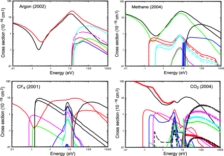
Figure 1: Cross sections of argon, CH₄, CF₄ and CO₂ as function of the electron energy [10]. See Refs. [10, 11] for each of the components contributing to the cross sections shown in curves.

From our experience $\sigma_{\rm X0}$ is about 50 $\mu$m (or better) for tracks perpendicular to the pad row direction if the charge spread in the amplification gap is not too small compared to the readout pad pitch and the S/N ratio of the readout electronics is good enough. The parameter $N_{\rm eff}$ has been measured to be around 20 in argon-based gases and for a pad height of $\sim$ 6 mm [5, 6], which is consistent with a simple estimate taking into account the primary ionization statistics and the avalanche fluctuation in the amplification gap [7].

If we require the azimuthal resolution of 100 $\mu$m at z = 200 cm the diffusion constant ($D$), which is essentially the only free (controllable) parameter depending on the choice of gas mixture, needs to be smaller than 30 $\mu$m/$\sqrt{\rm cm}$. The diffusion constant of drift electrons under the influence of an axial magnetic field ($B$) is given by

$$D(B)=D(B=0)/\sqrt{1+(\omega\tau)^{2}}\;,$$ (2)

where $\omega\equiv e\cdot B/m$, the electron cyclotron frequency, and $\tau$ is the mean free time of drift electrons between collisions with gas molecules. Therefore we need a gas mixture in which $D(B=0)$ is small (cool) and $\tau$ is fairly large (fast) under a moderate drift field ($E$).

A guideline to obtain a cool and fast gas is suggested by the deep and broad Ramsauer minimum in the electron cross section in argon, which is located around the electron energy ($\epsilon$) of 0.2 eV. It is necessary somehow to confine drift electrons near the Ramsauer minimum in argon, where the electrons are relatively cool and the cross section is small ($\tau$ is large), under a moderate drift field. Actually, argon itself is a very slow and hot gas and the drift electrons get hot quickly even under a weak drift field. Therefore it is necessary to add an efficient moderator, i.e. a small amount of molecular gas with its Ramsauer minimum at around $\epsilon$ = 0.2 eV and with large inelastic cross sections at $\epsilon\geq$ 0.2 eV in order to efficiently cool down relatively hot electrons [8, 9].

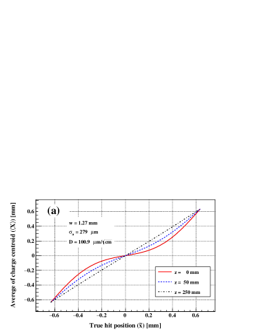
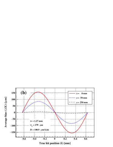
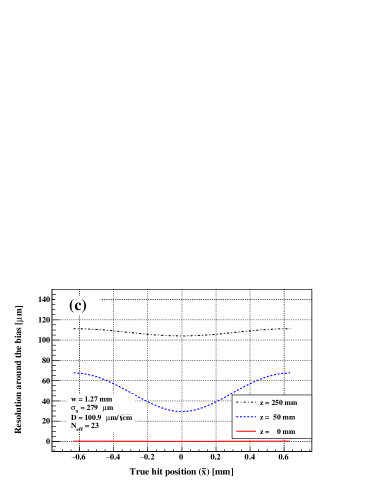
Figure 3: (a) Relation between the average of the charge centroid ($\left<X\right>$) and the true hit coordinate measured from the pad center ($\tilde{x}$). (b) Average bias ($\left<\Delta X\right>$) as a function of $\tilde{x}$. (c) Spatial resolution after bias subtraction as a function of $\tilde{x}$.

Good candidates for the additive gas are CH₄ and CF₄. The cross sections of relevant gases to electrons are seen in Fig. 3 as function of the electron energy. Figure 2 shows the mean electron energy as a function of the electric field for some pure gases and gas mixtures given by Magboltz [11]. All the results of Magboltz (version 8.5) presented in the present work are for gases at NTP (20^∘C, 1 atm). Examples of the electron energy distribution are shown in Fig. 3 for some gases of interest at several electric fields. The figure demonstrates that CH₄ or CF₄ molecules in argon are very efficient to keep the electron temperatures around those corresponding to the Ramsauer minimum, even under relatively high electric fields. Furthermore, CF₄ is superior to CH₄ as a moderator additive because of its much larger inelastic cross section to electrons with energies above the Ramsauer dip, due to vibrational excitation (see Fig. 1).

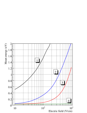
Figure 2: Mean electron energy as a function of the electric field given by Magboltz for (1) Ar (100%), (2) Ar-CH₄(5%), (3) Ar-CF₄(3%)-isobutane(2%), and (4) CO₂ (100%). Electrons are almost thermal in pure CO₂ in the range of electric field shown in the figure.

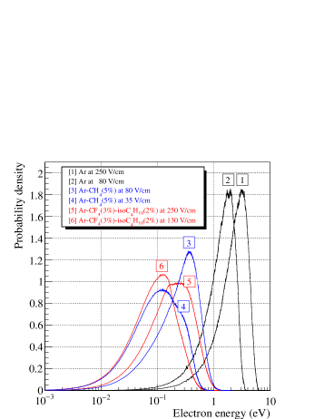
Figure 3: Electron energy distribution in some gases given by Magboltz. The electric field of 80 V/cm (250 V/cm) approximately corresponds to the drift-velocity maximum for Ar-CH₄(5%) (Ar-CF₄(3%)-isobutane(2%)) while the electric field of 35 V/cm (130 V/cm) corresponds to the diffusion minimum for Ar-CH₄(5%) (Ar-CF₄(3%)-isobutane(2%)).

Although they are fast and (relatively) cool themselves it is favorable to dilute them with argon in order to lower the drift field corresponding to the drift-velocity maximum by effectively reducing their inelastic cross sections, and at the same time, the operating high voltage of MPGDs. A low drift field is favorable especially for a large TPC in order to limit the high voltage for the central membrane to a moderate level. It is worth mentioning here that the drift field should be chosen so that the drift velocity be as close as possible to its maximum since the gas pressure in the LCTPC follows atmospheric pressure.

We have already tested several candidate gases, including TDR gas and P5 gas, for the LCTPC using a small prototype equipped with an MPGD (MicroMEGAS [13] or GEM [14]) in beam tests [5, 6]. The resultant transverse diffusion constants were always close to those given by Magboltz under 0 - 1 T magnetic fields. According to Magboltz the diffusion constant in P5 gas (TDR gas) at $B$ = 4 T, and $E\sim$ 80 V/cm ($\sim$ 220 V/cm) corresponding to the drift-velocity maximum, is about 40 $\mu$m/$\sqrt{\rm cm}$ (60 $\mu$m/$\sqrt{\rm cm}$) [15], which does not meet our requirement mentioned above.

As for Ar-CF₄, which is cooler and faster than P5 gas, we were not sure about the reliability of the Magboltz prediction although some measurements using prototype TPCs mainly equipped with MicroMEGAS exist [16, 17, 18, 19, 20, 21, 22]. We therefore conducted a series of cosmic ray tests using a small prototype TPC with a GEM readout operated in this possibly promising gas mixture of Ar-CF₄ (-isobutane) under a magnetic field of up to 1 T. In addition to the measurement of diffusion constant it was important as well to demonstrate successful operation of a GEM-equipped TPC in gases containing CF₄ since CF₄ molecules dissociatively capture relatively hot electrons in the vicinity of GEMs. It should be noted that the loss of drift electrons at the entrance to the first GEM could be fatal to the performance of a TPC, i.e. the spatial and the d$E$/d$x$ resolutions, since this loss can not be compensated by the subsequent gas multiplication.

The experimental setup is briefly described in Section 2. The results of gas gain measurements are given in Section 3, while the measured drift properties of the gas and the performance of the prototype are presented in Section 4. Section 5 is devoted to the conclusion.

2 Experimental setup

A photograph of the prototype (MP-TPC) is shown in Fig. 4.

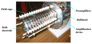
Figure 4: Photograph of the prototype just before installation into the gas vessel.

It consists of a field cage and an easily replaceable gas amplification device attached to one end of the field cage. Gas amplified electrons are detected by a pad plane at ground potential placed right behind the amplification device. A drift electrode is attached to the other end of the field cage. The maximum drift length is 257 mm.

In the present test a triple GEM is used as the amplification device. The triple GEM, CERN standard [26], has 1.5 mm transfer gaps and a 1.5 mm induction gap. The high voltages applied across each of the GEM foils and the transfer and induction gaps are set equal with a resistor-chain voltage divider.

The pad plane, with an effective area of $100\times 100$ mm², has 16 pad rows at a pitch of 6.3 mm, each consisting of $1.17\times 6$ mm² rectangular pads arranged at a pitch of 1.27 mm. The neighboring pad rows are staggered by half a pad pitch. Pad signals are fed to charge sensitive preamplifiers located 20 cm behind the bulkhead of the gas vessel. The amplified signals are sent to shaper amplifiers via twisted pair cables, and then processed by 12.5 MHz digitizers [27].

The chamber gases are mainly Ar-CF₄-isobutane mixtures at atmospheric pressure and room temperature. The gas pressure and the ambient temperature ($\sim 20^{\circ}$C) are periodically monitored since they are not controlled actively.

The prototype TPC is placed in the uniform field region of a superconducting solenoid without return yoke, having a bore diameter of 850 mm, an effective length of 1000 mm, and a maximum field strength of 1.2 T (see Fig. 5). A pair of scintillation counters sandwiching the prototype TPC is used to trigger a data acquisition system upon detection of cosmic ray tracks.

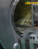
Figure 5: Photograph of the prototype ready to be inserted into the magnet.

The measurement of gas gain was carried out using a dedicated small test chamber and an ⁵⁵Fe source without magnetic field. The small chamber has a GEM stack with a configuration similar to that of the prototype TPC and a 10-mm drift gap for photon conversion with a field strength of 200 V/cm. Signal charge induced on its pad plane is read out by a combination of a preamplifier, a shaper amplifier and an analog to digital converter.

3 Gas gain measurements

A small value of the diffusion constant ($D\/$) and a reasonably large effective number of electrons ($N_{\rm eff}$) are crucial properties of the LCTPC gas as mentioned in Section 1. Another major practical issue is the gas gain in the amplification gap. The demonstration of stable operation of GEMs at an adequate gain is important particularly in a gas containing CF₄ since CF₄ molecules dissociatively attach hot electrons during their passage through the GEM stack. We therefore first measured the gas gains in several Ar-CF₄ based gas mixtures as function of the high voltage across each GEM foil (V_GEM). The electric fields in the transfer and the induction gaps were kept at 1.6 kV/cm throughout the measurements.

The results are shown in Fig. 6 for Ar-CF₄(3%) and Ar-CF₄(3%) with 2% admixture of methane, ethane, propane or isobutane. The gain obtained with a P10 gas (Ar-CH₄(10%)) is also included as a reference. Figure 7 gives the measured gas gain as a function of the isobutane content. The signal could not be observed without isobutane at V_GEM = 240 V.

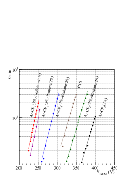
Figure 6: Measured gas gain as a function of GEM Voltage.

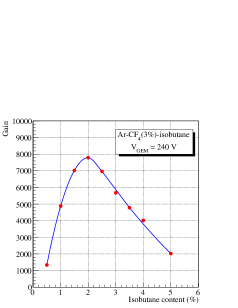
Figure 7: Measured gas gain as a function of isobutane concentration. Gas: Ar-CF₄(3%)-isobutane, V_GEM = 240 V. The curve is only to guide the eye.

The gain study shows that the addition of a small amount of isobutane (or propane) to Ar-CF₄ drastically lowers the operating GEM voltages which is required to obtain an adequate gas gain, as has already been found [17]. This is most likely due to the Penning effect since methane (ethane) is much less (moderately) effective as an additive gas. In addition, Magboltz shows that a small content of isobutane reduces the electron attachment by CF₄ molecules in the transfer/induction gaps by cooling down the migrating electrons, thereby increasing the effective gain of a GEM stack (see Fig. 8). It should be noted that high electric fields in the transfer and/or induction gaps could cause a significant loss of effective gain (even with isobutane). In the amplification region ($E\geq 10$ kV/cm) the gas multiplication dominates.

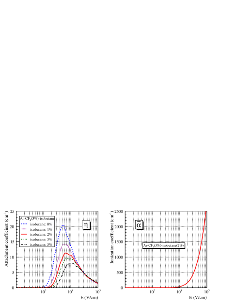
Figure 8: Attachment rates (left) and effective ionization coefficient (right) as function of the electric field given by Magboltz.

From the measurement above we decided to carry out the subsequent performance tests with the prototype TPC using a mixture of Ar-CF₄(3%)-isobutane(2%), with V_GEM = 240 V and the transfer and the induction fields of 1.6 kV/cm, resulting in an effective gas gain of $\sim$ 8000.

4 Performance of prototype

The data analysis of the recorded cosmic ray events was carried out using the traditional MultiFit (DoubleFit) program [28]. The hit coordinate on each pad row was determined by a simple charge centroid (barycenter) method using the pad signals within a charge cluster in the row, without any correction to the possible bias due to the finite pad pitch. Our major concern is the spatial resolution along the pad-row direction ($\sigma_{\rm X}$) since the requirement to the resolution along the drift direction ($\sigma_{\rm Z}$) is moderate for the LCTPC. The resolution $\sigma_{\rm Z}$ was measured to be 400 $\mu$m - 700 $\mu$m, depending on the drift distance and the drift-field strength.

We present in this section the drift properties of the gas and the performance of the prototype TPC obtained using cosmic rays nearly perpendicular ($\pm\;2^{\circ}$) to the readout pad rows and parallel ($\pm\;8^{\circ}$) to the pad plane, unless otherwise stated.

4.1 Drift properties

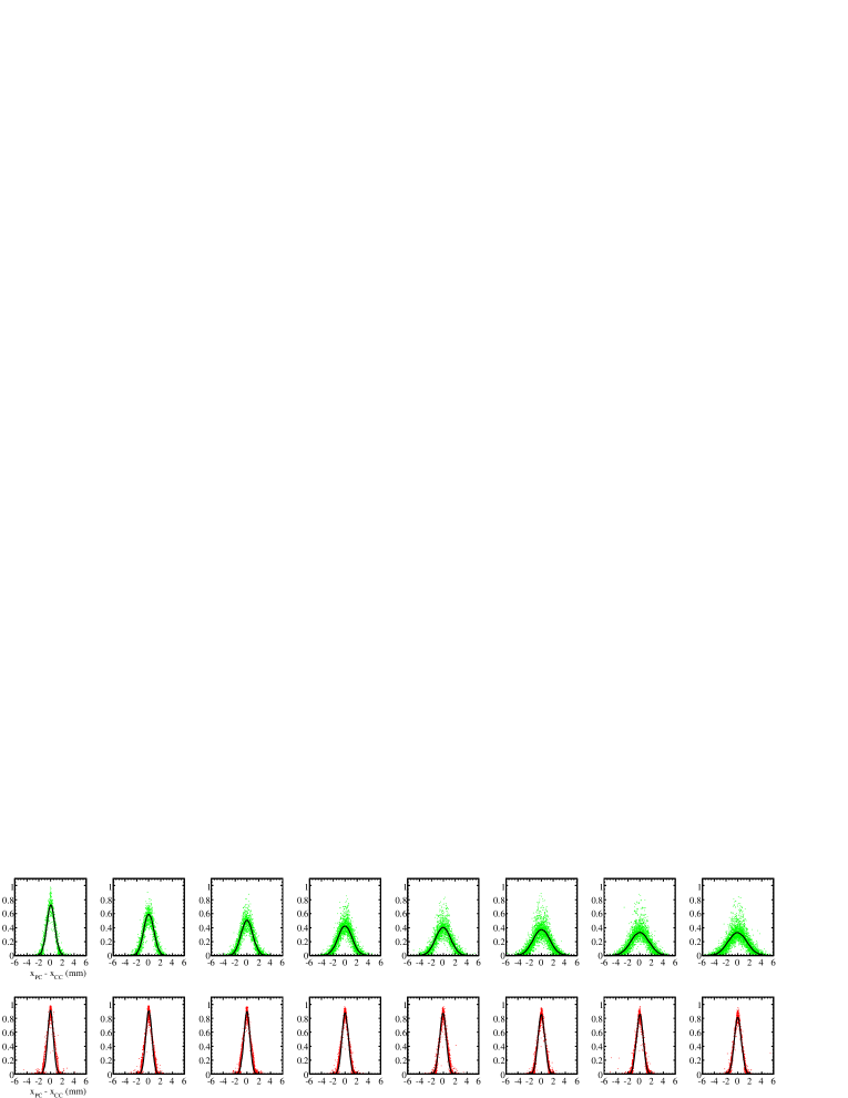
Figure 9: Pad responses for different drift distances, increasing from the left to the right up to 257 mm. The upper (lower) plots are for $B$ = 0 T ($B$ = 1 T). Gas: Ar-CF₄(3%)-isobutane(2%), Drift field: 130 V/cm. See text for the definitions of the horizontal and vertical axes. The solid curves represent the gaussians fitted through the data points.

Examples of the observed pad responses are plotted in Fig. 9, where the normalized charge on the pad ($q_{i}/\sum_{j}q_{j}$, with $q_{i}$ being the signal charge on pad $i\,$) is plotted against the distance of the pad center measured from the charge centroid, on a track by track basis. The data points are fitted with a gaussian (solid curve in the figure) in order to obtain the pad-response width for each region of the drift distance. Fig. 10 shows the pad-response width squared ($\sigma_{\rm PR}^{2}$) as a function of the drift distance ($z\/$) and a fitted straight line. The diffusion constants ($D\/$) were determined using the relation

$$\sigma_{\rm PR}^{2}=\sigma_{\rm PR0}^{2}+D^{2}\cdot z\;.$$ (3)

The constant term is given by

$$\sigma_{\rm PR0}^{2}=\frac{w^{2}}{12}+\sigma_{\rm PRF}^{2}\;,$$ (4)

where $w$ denotes the pad pitch (1.27 mm) and $\sigma_{\rm PRF}$ is the width of the avalanche-charge spread in the GEM stack along the pad row direction, for single drift electrons [6, 29]. The intersects of the fitted straight lines were always slightly larger than those calculated using Eq. (4) assuming the diffusion constants given by Magboltz in the transfer and induction gaps of the GEM stack to estimate $\sigma_{\rm PRF}$. The slopes of the fitted lines give the diffusion constants, which are summarized in Table 1 along with the measured drift velocities.

The drift velocity was determined from the full width of the drift-time distribution and the maximum drift length (257 mm). Figure 11 shows an example of the drift time distribution. The errors of the measured drift velocities were estimated conservatively assuming reading errors of $\pm$ 1 bin (80 nsec) both for the rising and falling edges of the distribution.

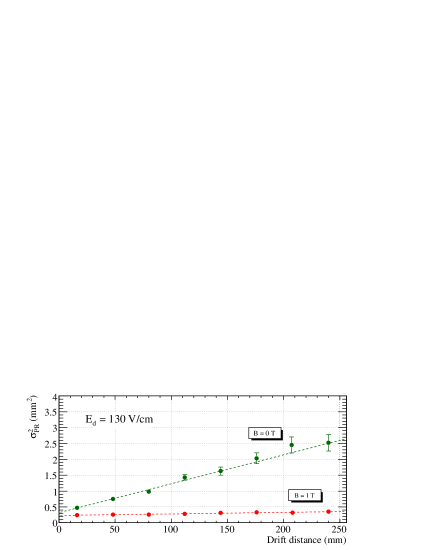
Figure 10: Pad-response width squared vs. drift distance. Gas: Ar-CF₄(3%)-isobutane(2%), Drift field: 130 V/cm.

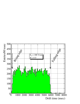
Figure 11: Drift time distribution. Gas: Ar-CF₄(3%)-isobutane(2%), Drift field: 100 V/cm, B = 0 T.

The measured drift properties are plotted in Fig. 12 along with the corresponding Magboltz predictions, which closely reproduce the data points. The reliability of Magboltz for this gas mixture was thus confirmed for the practical range of the electric field for TPC operation, i.e. between those corresponding to the diffusion minimum and the drift-velocity maximum.

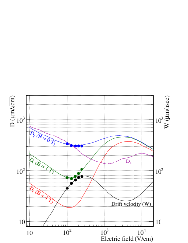
Figure 12: Measured transverse diffusion constants and drift velocities. Gas: Ar-CF₄(3%)-isobutane(2%). The Magboltz predictions (curves) are also shown for comparison.

Table 1: Drift properties and $N_{\rm eff}$ in Ar-CF₄(3%)-isobutane(2%)

(a) $B$ = 0 T
Drift velocity (cm/$\mu$s) Diffusion constant ($\mu$m/$\sqrt{{\rm cm}}$) $D/\sqrt{N_{{\rm eff}}}$ $E$ (V/cm) Measured Magboltz Measured Magboltz ($\mu$m/$\sqrt{{\rm cm}}$) $N_{\rm eff}$ 100 4.45 $\pm$ 0.13 4.50 337 $\pm$ 12 327.8 $\pm$ 2.4 74 $\pm$ 2 20.7 $\pm$ 1.8 130 5.67 $\pm$ 0.20 5.67 310 $\pm$ 11 316.7 $\pm$ 1.9 67 $\pm$ 2 21.1 $\pm$ 1.9 165 6.61 $\pm$ 0.28 6.69 305 $\pm$   8 311.7 $\pm$ 2.5 62 $\pm$ 2 24.1 $\pm$ 1.5 200 7.38 $\pm$ 0.34 7.35 306 $\pm$   8 311.2 $\pm$ 2.2 63 $\pm$ 2 23.8 $\pm$ 1.4 250 7.74 $\pm$ 0.38 7.81 305 $\pm$ 10 315.4 $\pm$ 2.4 65 $\pm$ 2 22.0 $\pm$ 1.8

(b) $B$ = 1 T
Drift velocity (cm/$\mu$s) Diffusion constant ($\mu$m/$\sqrt{{\rm cm}}$) $E$ (V/cm) Measured Magboltz Measured Magboltz 100 4.52 $\pm$ 0.13 4.50    72 $\pm$ 2   73.8 $\pm$ 0.7 130 5.74 $\pm$ 0.20 5.67    70 $\pm$ 2   72.8 $\pm$ 0.6 165 6.69 $\pm$ 0.28 6.69    77 $\pm$ 2   77.3 $\pm$ 0.6 200 7.30 $\pm$ 0.33 7.35    88 $\pm$ 2   85.5 $\pm$ 0.7 250 7.65 $\pm$ 0.36 7.81   106 $\pm$ 2 100.9 $\pm$ 0.7

4.2 Spatial resolution

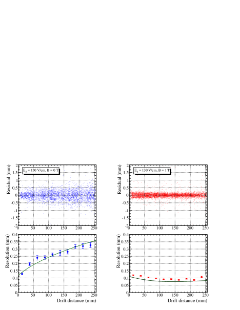
Figure 13: Geometric mean residual vs. drift distance for $B$ = 0 T (left) and $B$ = 1 T (right). Gas: Ar-CF₄(3%)-isobutane(2%), Drift field: 130 V/cm. The widths of the residuals are plotted against the drift distance in the lower figures, with a fitted curve (Eq. (1)) for $B$ = 0 T and a calculated resolution for $B$ = 1 T, respectively.

The spatial resolution along the pad row direction was obtained by plotting the geometric mean residuals against the drift distance on an event-by-event basis. A demonstration of the geometric mean method and the definition of the geometric mean residual are given in Appendix A. Figure 13 shows examples of the scatter plots thus obtained and the width along the ordinate axis as a function of the drift distance. In order to estimate the widths (standard deviations) the scatter plot was binned by drift distance and fitted by gaussians. The figures clearly show the improvement of the resolution due to a 1 T axial magnetic field. It should be noted that the resolution obtained with the magnetic field can not be fitted with Eq. (1) because of the degradation at small drift distances due to the finite pad-pitch effect. The curve shown in the figure for $B$ = 1 T is the result of the analytic calculation described in Appendix B and in Refs. [6, 29].

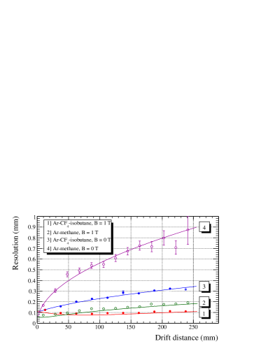
Figure 14: Spatial resolution vs. drift distance. Gas: Ar-CF₄(3%)-isobutane(2%), Drift field: 250 V/cm. Data points for P5 gas [5] are also plotted for comparison. Gas: Ar-CH₄(5%), Drift field: 100 V/cm. The curves in the figure are Eq. (1) fitted through the data points for $B$ = 0 T, and calculated resolutions for $B$ = 1 T.

In Fig. 14 the resolutions are compared to those measured previously with a P5 gas in the beam test [5] for drift fields corresponding approximately to the drift-velocity maxima. The figure shows the smaller degradation of the resolution at long drift distances due to diffusion in Ar-CF₄-isobutane. The effective numbers of electrons ($N_{\rm eff}$) for $B$ = 0 T listed in Table 1 were obtained readily from $D^{2}$ given by the pad response (Eq. (3)) and $D^{2}/N_{\rm eff}$ determined from the spatial resolution (Eq. (1)), as function of the drift distance. The average value of $N_{\rm eff}$ for Ar-CF₄(3%)-isobutane(2%) is $22.6\pm 1.5$, which should be compared to $22\pm 2$ obtained with a P5 gas [5]. All these values are comparable to an estimation [7]. It should be noted, however, that the apparent values of $N_{\rm eff}$ could be smaller than the true values because of electronic noise and inadequate calibration of the readout electronics (see Appendix C). Therefore the measured values are the lower limits of the genuine $N_{\rm eff}$ determined by the primary ionization statistics and the avalanche fluctuation.

As mentioned above it is difficult to deduce the value of $N_{\rm eff}$ using Eq. (1) for $B$ = 1 T because of the finite pad-pitch effect unless the drift region is long enough. Actually the observed resolution is the quadratic sum of the diffusion contribution, the finite pad-pitch term and a constant offset ($\sim\sigma_{\rm X0}$). The last term, which may depend on experimental conditions, can be estimated as the difference of the measured resolution squared and the calculated one.

As an example, each component contributing to the resolution is shown in Fig. 15 along with the measured resolution for $E_{\rm d}$ = 250 V/cm. In the calculation the diffusion constants in the drift region and in the transfer/induction gaps given by Magboltz were used. The value of $N_{\rm eff}$ was assumed to be 23. The constant offset is about (48 $\mu$m)² and is due most likely to electronic noise and inadequate calibration of the readout electronics. Possible major sources of the constant term are briefly discussed in Appendix C.

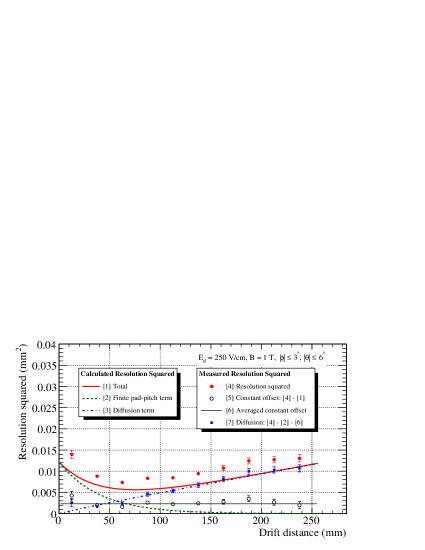
Figure 15: Spatial resolution squared vs. drift distance. Gas: Ar-CF₄(3%)-isobutane(2%), Drift field: 250 V/cm, $B$ = 1 T. The curves are the calculated resolution squared (solid line) and its components: the finite pad-pitch term (dashed line) and the diffusion term (dash-dotted line). The horizontal straight line represents the fitted constant offset.

The net diffusion contribution can thus be extracted by subtractions and is shown in filled squares in the figure. By fitting a straight line through those data points, $N_{\rm eff}$ under the 1 T magnetic field could be estimated. The resultant values are about 21 and 23, depending on the diffusion constant assumed, the Magboltz value (100.9 $\mu$m/$\sqrt{\rm cm}$) or the measured value (106 $\mu$m/$\sqrt{\rm cm}$). The values of $N_{\rm eff}$ thus obtained is consistent with those found from the resolutions in the absence of magnetic field (see Table 1), indicating that the effective number of electrons is not affected by the existence of the magnetic field as well as by the variation of the drift field.

5 Expected resolution of an LCTPC

Our measurements of the drift properties in Ar-CF₄(3%)-isobutane(2%) are well reproduced by the Magboltz code for $B$ = 0 and 1 T. This indicates that the cross sections of the gas molecules involved are correctly incorporated in the code at least for the corresponding electron energies for Ar-CF₄-isobutane seen in Fig. 3 and that the influence of the magnetic field on the transverse diffusion is properly included. Since the energy (random velocity) distribution of drifting electrons is not affected by the existence of axial magnetic field Magboltz is expected to give correct values of diffusion constants under stronger magnetic fields. In addition, the effective number of electrons is measured to be about 23 for the pad row pitch of 6.3 mm, which is affected little by the magnetic field if any. Therefore it is now possible to estimate the spatial resolution of the LCTPC using Eq. (12) in Appendix B.

Figure 16 shows the expected resolutions as function of the drift distance up to 2.5 m for a GEM-equipped LCTPC. In the calculation of the resolutions the transfer gaps and the induction gap of 4 mm are assumed for a triple GEM stack, with the electric fields in the gaps of 1600 V/cm while the drift field is set to 250 V/cm corresponding approximately to the drift-velocity maximum. The resolution better than 100 $\mu$m is thus feasible throughout the sensitive volume for tracks perpendicular to the pad row under an axial magnetic field of 4 T, at which the diffusion constant is predicted to be 29 $\mu$m/$\sqrt{\rm cm}$ by Magboltz, if the constant offset is kept reasonably small.

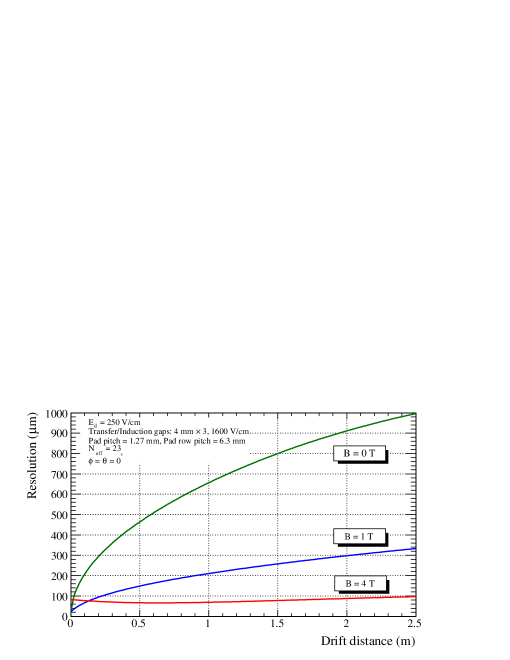
Figure 16: Expected spatial resolution of a GEM-equipped LCTPC for tracks perpendicular to the pad rows. Gas: Ar-CF₄(3%)-isobutane(2%), Drift field: 250 V/cm, $B$ = 4 T. The transfer and induction gaps are assumed to be 4 mm.

6 Conclusions

We have measured the diffusion constant, the drift velocity and the spatial resolution, as well as the gas gain, using a GEM-equipped TPC prototype operated in a gas mixture of Ar-CF₄(3%)-isobutane(2%) under magnetic fields of 0 T and 1 T. The prototype has been working stably with a sufficient gas gain in the cosmic ray test and gave a reasonable effective number of electrons ($N_{\rm eff}$), indicating a small loss, if any, of drift electrons at the entrance to the GEM stack. A reasonable value of $N_{\rm eff}$ means also that the gas-gain (avalanche) fluctuation is moderate. A small amount of isobutane ($\sim$ 2%) was found to be very effective to lower the operating high voltages of the GEMs, most likely due to the Penning effect.

The measured diffusion constants ($D$) in Ar-CF₄(3%)-isobutane(2%) are consistent with those given by Magboltz both for $B$ = 0 T and $B$ = 1 T, demonstrating the reliability of the Magboltz predictions for gas mixtures containing argon, CF₄ and isobutane. This gas mixture is confirmed to be cooler and faster than conventional TPC gases such as P5 and to ensure better azimuthal spatial resolution at long drift distances under a high axial magnetic field.

The spatial resolution better than 100 $\mu$m, the target of the LCTPC, is expected to be within reach with a GEM-based TPC operated in Ar-CF₄(3%) plus a small amount of isobutane under a 4 T magnetic field.

Appendix A Geometric mean method

In this appendix we give a simple demonstration of the geometric mean method applied in the analysis to estimate the spatial resolution.

First, in the case where the hit point in question (say, $x_{i}$, on the $i$-th pad row) is excluded in the track fitting, the residual is given by

$$\Delta x_{i}=x_{i}-\hat{x}_{i}\;,$$

where $\hat{x}_{i}$ represents the estimator for the $i$-th point given by the track fitting using the remaining hit points. Since $x_{i}$ and $\hat{x}_{i}$ are statistically independent the variance of the residual is given by

$$\sigma_{\rm excl}^{2} \equiv \left<(x_{i}-\hat{x}_{i})^{2}\right>-\left<x_{i}-\hat{x}_{i}\right>^{2}$$ (5)

$$= \left<x_{i}^{2}-2x_{i}\hat{x}_{i}+\hat{x}_{i}^{2}\right>-\left<x_{i}-\hat{x}_{i}\right>^{2}$$

$$= \left<x_{i}^{2}\right>-\left<x_{i}\right>^{2}+\left<\hat{x}_{i}^{2}\right>-\left<\hat{x}_{i}\right>^{2}$$

$$= \sigma_{x_{i}}^{2}+\sigma_{\hat{x}_{i}}^{2}\;,$$

the sum of the true spatial resolution and the tracking error.

Next, in the case where the hit point in question is included in the track fitting, the estimator for the $i$-th hit point is the weighted mean of $\hat{x}_{i}$ and $x_{i}$:

$$\hat{x}_{i}^{\prime}=\frac{w_{\hat{x}_{i}}\hat{x}_{i}+w_{x_{i}}x_{i}}{w_{\hat{x}_{i}}+w_{x_{i}}}\;,$$

with $w_{\hat{x}_{i}}$ $(w_{x_{i}})$ being the corresponding weight: $1/{\sigma_{\hat{x}_{i}}^{2}}$ $(1/{\sigma_{x_{i}}^{2}})$. The residual is hence given by

$$\Delta x_{i}^{\prime}\equiv x_{i}-\hat{x}_{i}^{\prime} = \frac{\sigma_{x_{i}}^{2}}{\sigma_{x_{i}}^{2}+\sigma_{\hat{x}_{i}}^{2}}(x_{i}-\hat{x}_{i})$$ (6)

$$= \frac{\sigma_{x_{i}}^{2}}{\sigma_{x_{i}}^{2}+\sigma_{\hat{x}_{i}}^{2}}\cdot\Delta x_{i}\;.$$

The variance of the residual in this case is therefore

$$\sigma_{\rm incl}^{2} \equiv \left<(x_{i}-\hat{x}_{i}^{\prime})^{2}\right>-\left<x_{i}-\hat{x}_{i}^{\prime}\right>^{2}$$ (7)

$$= \left(\frac{\sigma_{x_{i}}^{2}}{\sigma_{x_{i}}^{2}+\sigma_{\hat{x}_{i}}^{2}}\right)^{2}\cdot\left\{\left<(x_{i}-\hat{x}_{i})^{2}\right>-\left<x_{i}-\hat{x}_{i}\right>^{2}\right\}$$

$$= \left(\frac{\sigma_{x_{i}}^{2}}{\sigma_{x_{i}}^{2}+\sigma_{\hat{x}_{i}}^{2}}\right)^{2}\cdot\sigma_{\rm excl}^{2}\;.$$

Combining Eq. (5) and Eq. (7), the true spatial resolution is given by

$$\sigma_{x_{i}}=\sqrt{\sigma_{\rm excl}\cdot\sigma_{\rm incl}}\,.$$ (8)

Equation (8) demonstrates that the spatial resolution is obtained by taking the geometric mean of the two widths: one for the $\Delta x_{i}$ distribution and the other for the $\Delta x_{i}^{\prime}$ distribution. One may instead plot, on an event-by-event basis, geometric mean residuals defined as $\Delta x_{i}^{\prime\prime}\equiv S\cdot\sqrt{(x_{i}-\hat{x}_{i})\cdot(x_{i}-\hat{x}_{i}^{\prime})}\;,$ with $S$ being the sign of $x_{i}-\hat{x}_{i}$ (or equivalently $x_{i}-\hat{x}_{i}^{\prime}$  from Eq. (6)), and interpret its width as the spatial resolution since

$$\sigma_{\Delta x_{i}^{\prime\prime}}^{2} \equiv \left<S^{2}\cdot(x_{i}-\hat{x}_{i})\cdot(x_{i}-\hat{x}_{i}^{\prime})\right>$$

$$\hskip 28.45274pt-\left<S\cdot\sqrt{(x_{i}-\hat{x}_{i})\cdot(x_{i}-\hat{x}_{i}^{\prime})}\right>^{2}$$

$$= \frac{\sigma_{x_{i}}^{2}}{\sigma_{x_{i}}^{2}+\sigma_{\hat{x}_{i}}^{2}}\cdot\left\{\left<(x_{i}-\hat{x}_{i})^{2}\right>-\left<x_{i}-\hat{x}_{i}\right>^{2}\right\}$$

$$= \sigma_{x_{i}}^{2}\;.$$

Appendix B Analytic expression of the spatial resolution

One way to estimate the spatial resolution of a TPC along the pad-row direction is to write a realistic Monte-Carlo simulation code. This technique is applicable to any complicated situation, and has been developed by several groups. On the other hand, an analytic approach is applicable only to a restricted case where incident particles are normal to the pad row. However, the resultant formula is rather simple and is sometimes enlightening as shown below. Though a numerical calculation is needed to evaluate the formula, the demanded CPU time is much less than a Monte-Carlo simulation. In addition, the analytic calculation can be used to check the reliability of a Monte-Carlo simulation program, which is usually long and complicated. This appendix is devoted to briefly summarize our analytic approach, based on the following assumptions.

1. Particle tracks are normal to the pad row.

2. Track coordinate is determined by the charge centroid (barycenter) method.

3. Displacement of arriving drift electrons due to $E\times B$ effect near the entrance to the detection device is negligible.

4. Displacement of arriving electrons due to the finite granularity of amplification elements of the detection device (line intervals in MicroMEGAS or a hole pitch in GEM) is negligible.

B.1 Electronic noise contribution

Let us first consider the electronic noise contribution to the resolution degradation. The charge centroid of the signal including the noise is given by

$$X=\frac{1}{\sum_{j}(q_{j}+q_{j}^{\prime})}\cdot\sum_{j}(q_{j}+q_{j}^{\prime})x_{j}^{*}\;,$$

where $q_{j}$ ($q_{j}^{\prime}$ ) is the signal (noise) charge on pad $j$ and $x_{j}^{*}$ is the coordinate of the center of pad $j$. For simplicity we assume that $\sum_{j}q_{j}^{\prime}\ll\sum_{j}q_{j}$, therefore $\sum_{j}(q_{j}+q_{j}^{\prime})\approx\sum_{j}q_{j}$, and that $\bigl{<}q_{j}^{\prime}\bigr{>}=0$, $\bigl{<}q_{j}^{\prime}\cdot q_{k}^{\prime}\bigr{>}=\bigl{<}q^{\prime 2}\bigr{>}\cdot\delta_{jk}$ and $\bigl{<}q_{j}\cdot q_{k}^{\prime}\bigr{>}=0$. Then, with $\tilde{x}$ being the true track coordinate, the squared resolution along the pad-row direction is given by

$$\sigma_{X}^{2} = \bigl{<}(X-\tilde{x})^{2}\bigr{>}$$ (9)

$$= \biggl{<}\biggl{(}\frac{1}{\sum_{j}(q_{j}+q_{j}^{\prime})}\cdot\sum_{j}(q_{j}+q_{j}^{\prime})(x_{j}^{*}-\tilde{x})\biggr{)}^{2}\biggr{>}$$

$$= \biggl{<}\biggl{(}\frac{1}{\sum_{j}(q_{j}+q_{j}^{\prime})}\biggr{)}^{2}\cdot\biggl{(}\sum_{j}(q_{j}+q_{j}^{\prime})^{2}(x_{j}^{*}-\tilde{x})^{2}+\sum_{j\not\neq k}(q_{j}+q_{j}^{\prime})(q_{k}+q_{k}^{\prime})(x_{j}^{*}-\tilde{x})(x_{k}^{*}-\tilde{x})\biggr{)}\biggr{>}$$

$$\approx \biggl{<}\biggl{(}\frac{1}{\sum_{j}q_{j}}\biggr{)}^{2}\cdot\biggl{(}\sum_{j}(q_{j}^{2}+q_{j}^{\prime 2})(x_{j}^{*}-\tilde{x})^{2}+\sum_{j\not\neq k}q_{j}q_{k}(x_{j}^{*}-\tilde{x})(x_{k}^{*}-\tilde{x})\biggr{)}\biggr{>}$$

$$\approx \biggl{<}\biggl{(}\frac{1}{\sum_{j}q_{j}}\cdot\sum_{j}q_{j}(x_{j}^{*}-\tilde{x})\biggr{)}^{2}\biggr{>}+\biggl{<}\biggl{(}\frac{1}{\sum_{j}q_{j}}\biggr{)}^{2}\cdot\sum_{j}q_{j}^{\prime 2}(x_{j}^{*}-\tilde{x})^{2}\biggr{>}$$

$$\approx \biggl{<}\biggl{(}\frac{1}{\sum_{j}q_{j}}\cdot\sum_{j}q_{j}x_{j}^{*}-\tilde{x}\biggr{)}^{2}\biggr{>}+\biggl{<}\frac{1}{\bigl{(}\sum_{j}q_{j}\bigr{)}^{2}}\biggr{>}\cdot\bigl{<}q^{\prime 2}\bigr{>}\cdot\sum_{j}(x_{j}^{*}-\tilde{x})^{2}\;.$$

The second term represents the noise contribution whereas the first term gives the resolution obtained in the ideal case in which the electronic noise is absent.

Let us define $Q_{i}$ as the total gas-amplified signal charge on the pad row created by drift electron $i$. The total charge $Q_{i}$ is given by $\sum_{j}q_{ji}$, where $q_{ji}$ is the signal charge contribution of drift electron $i$, on pad $j$ ($q_{j}\equiv\sum_{i}q_{ji}$). Then $\sum_{j}q_{j}=\sum_{j}\sum_{i}q_{ji}=\sum_{i}Q_{i}$. Assuming that the total number of drift electrons per pad row ($N$, not a constant) is large enough

$$\sum_{j}q_{j}=\sum_{i=1}^{N}Q_{i}\approx N\cdot\bigl{<}Q\bigr{>}\;,$$

where $\bigl{<}Q\bigr{>}$ is the average total signal charge per drift electron.

Now the noise contribution is given by

$$\sigma_{X}^{2})_{\rm noise}\approx\biggl{<}\frac{1}{N^{2}}\biggr{>}\cdot\frac{\sigma_{q^{\prime}}^{2}}{\bigl{<}Q\bigr{>}^{2}}\cdot\sum_{j}(x_{j}^{*}-\tilde{x})^{2}\;.$$ (10)

This term increases with the signal charge spread along the pad row direction given by Eq. (3) because of the increase of the active number of pads (the summation range of $j$ around $\tilde{x}$). It should be noted that $x_{j}^{*}$ can be written as $j\cdot w$ with $w$ being the pad pitch.

B.2 Analytic evaluation of spatial resolution

In this section we evaluate the first term in Eq. (9). Let us redefine the charge centroid as follows.

$$X=\frac{\sum_{j}\sum_{i=1}^{N}q_{ji}\cdot x_{j}^{*}}{\sum_{j}\sum_{i=1}^{N}q_{ji}}\equiv\frac{\sum_{i=1}^{N}Q_{i}\sum_{j}F_{j}(x_{i})\cdot x_{j}^{*}}{\sum_{i=1}^{N}Q_{i}}\;,$$

where (see Fig. 1)

$$N : {\rm total~{}number~{}of~{}drift~{}electrons~{}per~{}pad~{}row},$$

$$x_{i} : {\rm arrival~{}position~{}of~{}electron}~{}i~{}{\rm at~{}the~{}entrance~{}to~{}the~{}detection~{}device},$$

$$x_{j}^{*} \equiv j\cdot w{\rm~{}~{}:~{}central~{}coordinate~{}of~{}pad~{}}j\;\;\;(j=\cdot\cdot\cdot,-2,-1,0,+1,+2,\cdot\cdot\cdot),$$

$$F_{j}(x_{i}) \equiv \frac{q_{ji}}{Q_{i}}\equiv\int_{jw-w/2}^{jw+w/2}f(\xi-x_{i})d\xi,$$

$$f(\xi) : {\rm(normalized)~{}pad~{}response~{}function~{}(PRF)}.$$

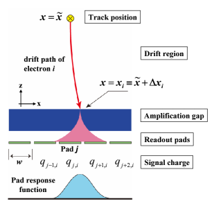
Figure 1: Illustration of the relevant variables.

It should be noted that the PRF here is determined solely by the charge spread in the detection gap and does not depend on the pad pitch whereas conventional PRFs do.

Then

$$\sigma_{X}^{2}(\tilde{x}) = \bigl{<}(X-\tilde{x})^{2}\bigr{>}$$

$$= \biggl{<}\biggl{(}\frac{\sum_{i=1}^{N}Q_{i}\sum_{j}F_{j}(x_{i})\cdot x_{j}^{*}}{\sum_{i=1}^{N}Q_{i}}-\tilde{x}\biggr{)}^{2}\biggr{>}$$

$$= \biggl{<}\biggl{(}\frac{\sum_{i=1}^{N}Q_{i}\sum_{j}F_{j}(x_{i})\cdot(x_{j}^{*}-\tilde{x})}{\sum_{i=1}^{N}Q_{i}}\biggr{)}^{2}\biggr{>}$$

$$= \biggl{<}\frac{1}{(\sum_{i}Q_{i})^{2}}\cdot\biggl{(}\sum_{i}Q_{i}^{2}\cdot\biggl{(}\sum_{j}F_{j}(x_{i})\cdot(x_{j}^{*}-\tilde{x})\biggr{)}^{2}$$

$$~{}~{}~{}~{}~{}~{}~{}~{}~{}~{}~{}~{}~{}~{}~{}~{}~{}~{}~{}~{}+\sum_{i\neq l}Q_{i}Q_{l}\cdot\biggl{(}\sum_{k}F_{k}(x_{i})\cdot(x_{k}^{*}-\tilde{x})\sum_{k}F_{k}(x_{l})\cdot(x_{k}^{*}-\tilde{x})\biggr{)}\biggr{)}\biggr{>}$$

$$= \biggl{<}\frac{1}{(\sum_{i}Q_{i})^{2}}\cdot\biggl{(}\sum_{i}Q_{i}^{2}\cdot\Bigl{(}\sum_{j}F_{j}(x_{i})\cdot x_{j}^{*}-\tilde{x}\Bigr{)}^{2}$$

$$~{}~{}~{}~{}~{}~{}~{}~{}~{}~{}~{}~{}~{}~{}~{}~{}~{}~{}~{}~{}+\sum_{i\neq l}Q_{i}Q_{l}\cdot\biggl{(}\Bigl{(}\sum_{k}F_{k}(x_{i})\cdot x_{k}^{*}-\tilde{x}\Bigr{)}\Bigl{(}\sum_{k}F_{k}(x_{l})\cdot x_{k}^{*}-\tilde{x}\Bigr{)}\biggr{)}\biggr{)}\biggr{>}$$

$$= \biggl{<}\frac{1}{(\sum_{i}Q_{i})^{2}}\cdot\biggl{(}\sum_{i}Q_{i}^{2}\cdot\biggl{<}\Bigl{(}\sum_{j}F_{j}(x)\cdot x_{j}^{*}-\tilde{x}\Bigr{)}^{2}\biggr{>}_{x}$$

$$~{}~{}~{}~{}~{}~{}~{}~{}~{}~{}~{}~{}~{}~{}~{}~{}~{}~{}~{}~{}~{}~{}~{}~{}~{}~{}~{}~{}~{}~{}~{}~{}~{}~{}~{}+\bigl{(}\sum_{i,l}Q_{i}Q_{l}-\sum_{i}Q_{i}^{2}\bigr{)}\cdot\biggl{<}\sum_{k}F_{k}(x)\cdot x_{k}^{*}-\tilde{x}\biggr{>}_{x}^{2}~{}\biggr{)}\biggr{>}_{Q}$$

$$= \biggl{<}\sum_{j}F_{j}(x)\cdot x_{j}^{*}-\tilde{x}\biggr{>}_{x}^{2}+\biggl{<}\frac{\sum_{i}Q_{i}^{2}}{(\sum_{i}Q_{i})^{2}}\biggr{>}_{Q}\cdot\biggl{(}\biggl{<}\sum_{j,k}F_{j}(x)\cdot F_{k}(x)\cdot x_{j}^{*}\cdot x_{k}^{*}\biggr{>}_{x}-\biggl{<}\sum_{j}F_{j}(x)\cdot x_{j}^{*}\biggr{>}_{x}^{2}~{}\biggr{)}$$

$$= \biggl{(}\sum_{j}\bigl{<}F_{j}(x)\bigr{>}\cdot x_{j}^{*}-\tilde{x}\biggr{)}^{2}+\biggl{<}\frac{\sum_{i}Q_{i}^{2}}{(\sum_{i}Q_{i})^{2}}\biggr{>}\cdot\biggl{(}\sum_{j,k}\bigl{<}F_{j}(x)\cdot F_{k}(x)\bigr{>}\cdot x_{j}^{*}\cdot x_{k}^{*}-\biggl{(}\sum_{j}\bigl{<}F_{j}(x)\bigr{>}\cdot x_{j}^{*}\biggr{)}^{2}~{}\biggr{)}$$

$$\approx \biggl{(}\sum_{j}\bigl{<}F_{j}(x)\bigr{>}\cdot x_{j}^{*}-\tilde{x}\biggr{)}^{2}+\frac{1}{N}\cdot\frac{\bigl{<}Q^{2}\bigr{>}}{\bigl{<}Q\bigr{>}^{2}}\cdot\biggl{(}\sum_{j,k}\bigl{<}F_{j}(x)\cdot F_{k}(x)\bigr{>}\cdot x_{j}^{*}\cdot x_{k}^{*}-\biggl{(}\sum_{j}\bigl{<}F_{j}(x)\bigr{>}\cdot x_{j}^{*}\biggr{)}^{2}~{}\biggr{)}\;.$$

In the last line $\sum_{i}Q_{i}$ is approximated by $N\cdot\left<Q\right>$, assuming large $N$. Averaging over $N$ and substituting $j\cdot w$ and $k\cdot w$, respectively for $x_{j}^{*}$ and $x_{k}^{*}$ we get

$$\sigma_{X}^{2}(\tilde{x})\approx\biggl{(}\sum_{j}jw\cdot\bigl{<}F_{j}(x)\bigr{>}-\tilde{x}\biggr{)}^{2}+\frac{1}{N_{\rm eff}}\cdot\biggl{(}\sum_{j,k}jkw^{2}\cdot\bigl{<}F_{j}(x)\cdot F_{k}(x)\bigr{>}-\biggl{(}\sum_{j}jw\cdot\bigl{<}F_{j}(x)\bigr{>}\biggr{)}^{2}~{}\biggr{)}\;,\\$$ (11)

where

$$\frac{1}{N_{\rm eff}}\equiv\biggl{<}\frac{1}{N}\biggr{>}\cdot\frac{\bigl{<}Q^{2}\bigr{>}}{\bigl{<}Q\bigr{>}^{2}}=\biggl{<}\frac{1}{N}\biggr{>}\cdot\biggl{(}1+\frac{\sigma_{Q}^{2}}{\bigl{<}Q\bigr{>}^{2}}\biggr{)}\;,$$

$$\bigl{<}F_{j}(x)\bigr{>}\equiv\int_{-\infty}^{\infty}P_{x}(x)\cdot F_{j}(x)\;dx\;,\hskip 256.0748pt$$

$$\bigl{<}F_{j}(x)\cdot F_{k}(x)\bigr{>}\equiv\int_{-\infty}^{\infty}P_{x}(x)\cdot F_{j}(x)\cdot F_{k}(x)\;dx\;,$$

$${\rm with}$$

$$P_{x}(x)\equiv\frac{1}{\sqrt{2\pi}\sigma_{d}}{\rm exp}\biggl{(}-\frac{(x-\tilde{x})^{2}}{2\sigma_{d}^{2}}\biggr{)}\;,$$

$$F_{j}(x)\equiv\int_{jw-w/2}^{jw+w/2}f(\xi-x)\,d\xi\;,$$

$$f(\xi):{\rm~{}PRF}\;.$$

The parameter $\sigma_{d}$ in the definition of $P_{x}(x)$ denotes the (lateral) standard deviation of the arrival position of drift electrons at the entrance to the amplification device measured from $\tilde{x}$, and is given by $D\cdot\sqrt{z}$.

Hence the spatial resolution as a function of the drift distance ($z$) can be numerically evaluated once the pad pitch ($w$), the diffusion constant ($D$), the pad response function ($f$), and the effective number of electrons ($N_{\rm eff}$) are given. In our case the pad response function is assumed to be a gaussian

$$f(\xi)=\frac{1}{\sqrt{2\pi}\sigma_{a}}{\rm exp}\biggl{(}-\frac{\xi^{2}}{2\sigma_{a}^{2}}\biggr{)}\;,$$

with $\sigma_{a}$ being the charge spread in the GEM stack.

Though Eq. (11) may appear a little complicated its meaning is quite simple: the first term is the bias inherent in the charge centroid method (finite pad-pitch term) while the second term represents the variance around the bias, divided by $N_{\rm eff}$ (diffusion term). This is shown clearly by rewriting Eq. (11) as

$$\sigma_{X}^{2}(\tilde{x})\approx\biggl{<}\sum_{j}F_{j}(x)\cdot x_{j}^{*}-\tilde{x}\biggr{>}^{2}+\frac{1}{N_{\rm eff}}\biggl{<}\biggl{(}\sum_{j}F_{j}(x)\cdot x_{j}^{*}-\biggl{<}\sum_{j}F_{j}(x)\cdot x_{j}^{*}\biggr{>}\biggr{)}^{2}~{}\biggr{>}\;.$$

It should be pointed out here that $\sigma_{X}^{2}$ depends on the position of $\tilde{x}$ relative to the corresponding pad center, and that the beam spot size is usually much larger than the pad pitch. Therefore unless the incident positions of incoming particles are measured precisely by external trackers (e.g. by a set of silicon strip detectors) on an event-by-event basis, $\sigma_{X}^{2}(\tilde{x})$ obtained above (Eq. (11)) has to be averaged over $\tilde{x}$ in a range, say, [-$w$/2, +$w$/2]:

$$\sigma_{X}^{2}=\frac{1}{w}\cdot\int_{-w/2}^{+w/2}\sigma_{X}^{2}(\tilde{x})\;d\tilde{x}\;.$$

In order to see the asymptotic behavior of the resolution it is convenient to rewrite Eq. (11):

$$\sigma_{X}^{2}(\tilde{x})\approx\biggl{<}\sum_{j}F_{j}(x)\cdot x_{j}^{*}-\tilde{x}\biggr{>}^{2}+\frac{1}{N_{\rm eff}}\biggr{(}\biggl{<}\biggl{(}\sum_{j}F_{j}(x)\cdot x_{j}^{*}-\tilde{x}\biggr{)}^{2}\biggr{>}-\biggl{<}\sum_{j}F_{j}(x)\cdot x_{j}^{*}-\tilde{x}\biggr{>}^{2}\biggr{)}\;,$$

and define

$$\sigma_{X}^{2}=\frac{1}{w}\cdot\int_{-w/2}^{w/2}\sigma_{X}^{2}(\tilde{x})\;d\tilde{x}\approx B^{2}+\frac{1}{N_{\rm eff}}\cdot(A^{2}-B^{2})\;,$$ (12)

where

$$B^{2} \equiv \frac{1}{w}\cdot\int_{-w/2}^{w/2}\biggl{<}\sum_{j}F_{j}(x)\cdot x_{j}^{*}-\tilde{x}\biggr{>}^{2}\;d\tilde{x}\;,$$

$$A^{2} \equiv \frac{1}{w}\cdot\int_{-w/2}^{w/2}\biggl{<}\biggl{(}\sum_{j}F_{j}(x)\cdot x_{j}^{*}-\tilde{x}\biggr{)}^{2}\biggr{>}\;d\tilde{x}\;.$$

The term $B^{2}$ vanishes in the limit $\sigma_{d}\rightarrow\infty\;(z\rightarrow\infty)$ since $\sum_{j}\left<F_{j}(x)\right>x_{j}^{*}\rightarrow\tilde{x}$ for any given $\tilde{x}$ while the term $A^{2}$ can easily be shown to be $B_{0}^{2}+\sigma_{d}^{2}=B_{0}^{2}+D^{2}\cdot z$, where $B_{0}^{2}\equiv B^{2}\;]_{\sigma_{d}=0}=B^{2}\;]_{z=0}$. Therefore

$$\sigma_{X}^{2}\rightarrow\frac{1}{N_{\rm eff}}\cdot\bigl{(}B_{0}^{2}+D^{2}\cdot z\bigr{)}$$ (13)

at long drift distances.

Figure 2 shows an example of the calculated resolution in our case. In the calculation the following values were assumed: $w$ = 1.27 mm, $\sigma_{a}$ = 279 $\mu$m, $D$ = 100.9 $\mu$m/$\sqrt{\rm cm}$ (Magboltz value), and $N_{\rm eff}$ = 23. $\sigma_{a}$ was estimated using the diffusion constant in the transfer and the induction gaps given by Magboltz. The dashed straight line shows the asymptotic behavior at long drift distances (Eq. (13)), which has an offset of $B_{0}^{2}/N_{\rm eff}\approx(23\;\mu{\rm m})^{2}$. This is the fundamental lower limit of the constant contribution to the spatial resolution ($\sigma_{\rm X0}^{2}$), determined by the pad pitch ($w$), the charge spread in the detection gap ($\sigma_{a}$), and the effective number of electrons ($N_{\rm eff}$).

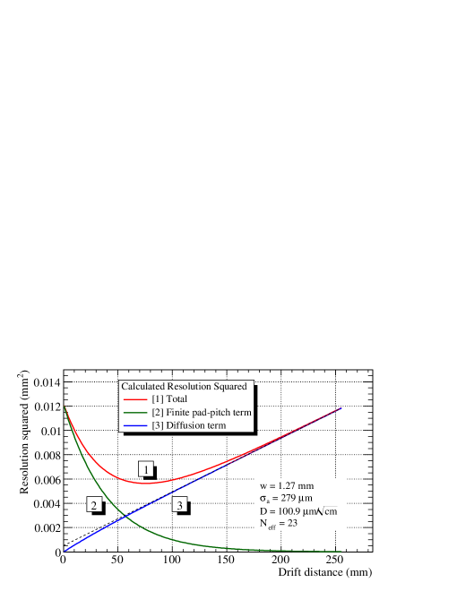
Figure 2: Calculated resolution squared for $E_{\rm d}$ = 250 V/cm and $B$ = 1 T. See text for the dashed line.

Appendix C Contributors to the constant term

In this appendix we qualitatively discuss the origin of the constant term contained in the spatial resolution ($\sigma_{\rm X0}^{2}$) in our case. Possible main sources of the constant term are listed below for tracks perpendicular to the pad-row direction.

1. Intrinsic track width ($\delta$-rays) [30].

2. Multiple Coulomb scattering.

3. Mechanical imprecision.

4. Influence of the finite hole pitch of the GEM foils.

5. Influence of the finite pad pitch.

6. Electronic noise.

7. Inadequate calibration of the readout electronics, such as channel-to-channel (pad-to-pad) inequalities of the gain and inappropriate pedestal subtractions from the raw signals.

The sources (1) and (2) are intrinsic and unavoidable while the others can be made sufficiently small in principle.

The intrinsic track width certainly contributes to the constant term. The value of $\sigma_{\rm X0}^{2}$ obtained with the magnetic field ($\sim$ (50 $\mu$m)²) is significantly smaller than those for the resolutions obtained without the magnetic field ($\sim$ (100 $\mu$m)², see Figs. 13 and 14 for example) because of the suppression of the transverse intrinsic track width by the axial magnetic field. The magnetic field reduces the effective range of $\delta$-rays along the pad-row direction.

The mechanical precision such as the readout pad arrangement is expected to be good enough. The influence of the hole pitch of the GEM foils (horizontal pitch of 140 $\mu$m) was also found to be small by means of a Monte-Carlo simulation (see, for example, Fig. 4 of Ref. [5]). The constant term (at long drift distances) is caused by the finite pad pitch as well (see Appendix B, Eq. (13)). However, its contribution is small in our case, (18 $\mu$m)² - (23 $\mu$m)², depending on the magnetic field (0 T - 1 T).

The contribution of the angular pad effect for the azimuthal angle cut of $\pm$ 3^∘ was estimated to be $\sim$ (20 $\mu$m)² by a Monte Carlo simulation. Therefore the main contributors to $\sigma_{\rm X0}^{2}$ are expected to be (6) and (7), except for the unavoidable contribution from (1) and (2).

The sources (6) and (7) have contribution increasing with the drift distance ($z$) as well as a constant term at $z$ = 0 because of the increase of the number of active pads used to determine the charge centroid, due to diffusion (see Figs. 9 and 10, and Eq. (10) for the contribution of electronic noise). Therefore they can affect the apparent value of $N_{\rm eff}$ as well.

Addendum to be published in Nucl. Instrum. Methods Phys. Res. A

The finite pad-pitch term shown in Fig. B2 in Appendix B can be eliminated, if not completely, provided that the charge spread in the GEM stack ($\sigma_{a}$) is not too small compared to the pad pitch ($w$) and the electronic noise is small enough so that the threshold for the flash ADCs is set low enough. It corresponds to the first term in Eq. (B.3) and the following equivalent equations, that represents the bias inherent in the charge centroid (barycenter) method used to get the track coordinate at a pad row ($X$). The average bias ($\left<\Delta X\right>$) is a function of the true hit coordinate $\tilde{x}$ (measured from the center of the pad with the maximum charge deposit). It depends also on the drift distance ($z$) since the lateral diffusion of drift electrons ($\sigma_{d}$) is expressed as

$$\sigma_{d}=D\cdot\sqrt{z}$$ (14)

where $D$ denotes the transverse diffusion constant.

The average bias is the first term of Eq. (B.3) before squared:

$$\left<\Delta X(\tilde{x})\right>\equiv\left<X\right>-\tilde{x}\equiv\sum_{j}\;j\cdot w\cdot\left<F_{j}(x)\right>-\tilde{x}$$ (15)

where

$$\bigl{<}F_{j}(x)\bigr{>}\equiv\int_{-\infty}^{\infty}P_{x}(x)\cdot F_{j}(x)\;dx$$ (16)

$$P_{x}(x)\equiv\frac{1}{\sqrt{2\pi}\sigma_{d}}{\rm exp}\biggl{(}-\frac{(x-\tilde{x})^{2}}{2\sigma_{d}^{2}}\biggr{)}$$ (17)

$$F_{j}(x)\equiv\int_{jw-w/2}^{jw+w/2}f(\xi-x)\,d\xi$$ (18)

$$f(\xi)\equiv\frac{1}{\sqrt{2\pi}\sigma_{a}}{\rm exp}\biggl{(}-\frac{\xi^{2}}{2\sigma_{a}^{2}}\biggr{)}$$ (19)

with $j$ ($w$), the pad number (pad pitch).

The value of $\left<F_{j}(x)\right>$ can be calculated for a given $\tilde{x}$ if $\sigma_{a}$, $D$, and $z$ (drift time) are known. One can thus obtain a one-to-one correspondence between $\left<X\right>$ and $\tilde{x}$. Therefore, the value of $X$ given by the charge centroid method can be projected onto a bias-free estimate of $\tilde{x}$, assuming $X=\left<X\right>$. Although the projection is not perfect because of fluctuations of $X$ around $\left<X\right>$, it is the simplest way of removing the bias without relying on the tracking information provided by the other pad rows.

Fig. 1(a) shows the relation between $\tilde{x}$ and $\left<X\right>$. Fig. 1(b) shows the average bias ($\left<\Delta X\right>$) given by Eq. (2) as a function of $\tilde{x}$ measured from the pad center, while Fig. 1(c) is the spatial resolution, after the bias subtraction, as a function of $\tilde{x}$, i.e. the square root of the second term of Eq. (B.3).

Fig. 1(c) shows that the charge centroid after the perfect bias subtraction always gives the true coordinate ($\tilde{x}$) at $z$ = 0. The second term in Eq. (B.3) vanishes at $z$ = 0 for any $\tilde{x}$ because of the assumptions (3)–(5) listed at the beginning of Appendix B. In the case of GEMs, the item (4) means an infinitesimal hole pitch. Consequently, the second term of Eq. (B.4) (diffusion term) vanishes at $z$ = 0, as shown in Fig. B2. The diffusion term is the square of such as that shown in Fig. 1(c) averaged over $\tilde{x}$ for the corresponding drift distance ($z$).

It should be noted that the fluctuations of the charge centroid of multiplied electrons in the GEM stack for a single drift electron are small when the effective gain of the first GEM is large enough. Their contribution to the diffusion term is further reduced by the factor $N_{\rm eff}$.

It should also be noted that the contribution of electronic noise (Eq. (B.2)) is neglected assuming a large gas gain in the GEM stack. See Appendix C for other possible sources of the degradation of the spatial resolution.

By definition, the diffusion term depends on the pad pitch ($w$) as well as the drift distance ($z$). It is, therefore, appropriate to call the first (second) term of Eq. (B.4) bias (statistical fluctuation) term independent of (dependent on) $N_{\rm eff}$.

References

-
[1]
The International Linear Collider: ILC Reference Design Report,
available at http://www.linearcollider.org/rdr. -
[2]
The Compact Linear Collider: The Compact Linear Collider Study,
http://clic-study.web.cern.ch/CLIC-Study/. - [3] D. Nygren, The Time-Projection Chamber - 1975, PEP-198 (1975).
-
[4]
K. Ackermann, et al.,
Cosmic Ray Tests of the Prototype TPC for the ILC Experiment,
arXiv:0905.2655 [physics.ins-det];
K. Ackermann, et al., Nucl. Instr. and Meth. A 623 (2010) 141. -
[5]
M. Kobayashi, et al.,
Nucl. Instr. and Meth. A 581 (2007) 265;
M. Kobayashi, et al., Nucl. Instr. and Meth. A 584 (2008) 444. - [6] D.C. Arogancia, et al., Nucl. Instr. and Meth. A 602 (2009) 403.
- [7] M. Kobayashi, Nucl. Instr. and Meth. A 562 (2006) 136.
- [8] L.G. Christophorou, D.L. McCorkle, D.V. Maxey and J.G. Carter, Nucl. Instr. and Meth. 163 (1979) 141.
- [9] L.G. Christophorou, P.G. Datskos and J.G. Carter, Nucl. Instr. and Meth. A 309 (1991) 160.
- [10] http://consult.cern.ch/writeup/magboltz/.
- [11] S.F. Biagi, Nucl. Instr. and Meth. A 421 (1999) 234.
- [12] L. G. H. Huxley and R. W. Crompton, The Diffusion and Drift of Electrons in Gases, Wiley, New York, 1974 (Chapter 3).
- [13] Y. Giomataris, et al., Nucl. Instr. and Meth. A 376 (1996) 29.
- [14] F. Sauli, Nucl. Instr. and Meth. A 386 (1997) 531.
- [15] See http://www-hep.phys.saga-u.ac.jp/ILC-TPC/gas/ for the drift properties of a variety of gas mixtures given by Magboltz.
- [16] P. Colas, et al., Nucl. Instr. and Meth. A 535 (2004) 181.
- [17] D. Attié, et al., Gas issues for a Micromegas TPC for the Future Linear Collider, Talk presented at the Endplate Meeting, Paris, September 2006.
- [18] E. Radicioni, et al., A GEM based TPC with two large 3-GEM Towers, IEEE NSS Conference Record (2006) 3842 (MP3-3).
- [19] The T2K ND280 TPC Group, T2K ND280 TPC Technical Design Report, T2K Internal Document (2007).
- [20] J. Bouchez, et al., Nucl. Instr. and Meth. A 574 (2007) 425.
- [21] M. Dixit, et al., Nucl. Instr. and Meth. A 581 (2007) 254.
- [22] S.X. Oda, et al., Nucl. Instr. and Meth. A 566 (2006) 312.
- [23] R. Thun, Nucl. Instr. and Meth. A 273 (1988) 157.
- [24] W.S. Anderson, et al., Nucl. Instr. and Meth. A 323 (1992) 273.
- [25] T. Isobe, et al., Nucl. Instr. and Meth. A 564 (2006) 190.
- [26] S. Bachmann, et al., Nucl. Instr. and Meth. A 433 (1999) 464.
- [27] M. Ball, N. Ghodbane, M. Janssen and P. Wienemann, A DAQ System for Linear Collider TPC Prototypes based on the ALEPH TPC Electronics, arXiv:physics/0407120 [physics.ins-det].
- [28] M. E. Janssen (on behalf of the FLC-TPC group at DESY), R&D Ongoing at DESY for a GEM based TPC at the ILC: Resolution Studies; Techniques and Results, IEEE Nuclear Science Symposium Conference Record (2006) pp. 38-42 (N04-4), and references cited therein.
- [29] M. Kobayashi, et al., A Beam test of Prototype TPCs Using Micro-Pattern Gas Detectors at KEK, KEK Preprint 2006-35 (KISS Accession No. 200627035).
- [30] F. Sauli, Nucl. Instr. and Meth. 156 (1978) 147.