Effective boundary condition at a rough surface
starting from a slip condition

Abstract

We consider the homogenization of the Navier-Stokes equation, set in a channel with a rough boundary, of small amplitude and wavelength $\epsilon$. It was shown recently that, for any non-degenerate roughness pattern, and for any reasonable condition imposed at the rough boundary, the homogenized boundary condition in the limit ${\varepsilon}=0$ is always no-slip. We give in this paper error estimates for this homogenized no-slip condition, and provide a more accurate effective boundary condition, of Navier type. Our result extends those obtained in [6, 13], in which the special case of a Dirichlet condition at the rough boundary was examined.

Keywords: Wall laws, rough boundaries, homogenization, ergodicity, Korn inequality

1 Introduction

Most works on Newtonian liquids assume the validity of the no-slip boundary condition: the velocity field of the liquid at a solid surface equals the velocity field of the surface itself. This assumption relies on both theoretical and experimental studies, carried over more than a century.

Still, with the recent surge of activity around microfluidics, the question of fluid-solid interaction has been reconsidered, and the consensus around the no-slip condition has been questioned. Several experimentalists, observing for instance water over mica, have reported significant slip. More generally, it has been claimed that, in many cases, the liquid velocity field $u$ obeys a Navier condition at the solid boundary $\Sigma$:

$$(I_{d}-\nu\otimes\nu)u|_{\Sigma}\>=\>\lambda(I_{d}-\nu\otimes\nu)D(u)\nu|_{\Sigma},\quad u\cdot\nu|_{\Sigma}\>=\>0,\quad\lambda>0$$ (Na)

where $\nu$ is an inward normal vector to $\Sigma$, and $D(u)$ is the symmetric part of the gradient. Slip lengths $\lambda$ up to a few micrometers have been measured. This is far more than the molecular scale, and would therefore invalidate the (macroscopic) no-slip condition

$$u|_{\Sigma}=0.$$ (Di)

Nevertheless, such experimental results are widely debated. For similar experimental settings, there are huge discrepancies between the measured values of $\lambda$. We refer to the article [18] for an overview.

In this debate around boundary conditions, the irregularity of the solid surface is a major issue. Again, its effect is a topic of intense discussion. On one hand, some people argue that it increases the surface of friction, and may cause a decrease of the slip. On the other hand, it may generate small scale phenomena favourable to slip. For instance, some rough hydrophobic surfaces seem more slippery due to the trapping of air bubbles in the humps of the roughness. Moreover, irregularity creates a boundary layer in its vicinity, meaning high velocity gradients. Thus, even though (Di) is satisfied at the rough boundary, there may be significant velocities right above. In other words, the no-slip condition may hold at the small scale of the boundary layer but not at the large scale of the mean flow. This phenomenon, due to scale separation, is called apparent slip in the physics litterature.

In parallel to experimental works, several theoretical studies have been carried, so as to clarify the role of roughness. Many of them relate to homogenization theory. First, the irregularity is modeled by small-scale variations of the boundary. Then, an asymptotic analysis is performed, as the small scales go to zero. The idea is to replace the constitutive boundary condition at the rough surface by a homogenized or effective boundary condition at the smoothened surface. In this way, one can describe the averaged effect of the roughness. We stress that such homogenized conditions (often called wall laws) are also of practical interest in numerical codes. They allow to filter out the small scales of the boundary, which have a high computational cost.

Let us recall briefly the main mathematical results on wall laws. To give a unified description, we take a single model. Namely, we consider a two-dimensional rough channel

$$\Omega^{\varepsilon}\>:=\>\Omega\cup\Sigma\cup R^{\varepsilon}$$

where $\Omega={\mathbb{R}}\times(0,1)$ is the smooth part, $R^{\varepsilon}$ is the rough part, and $\Sigma={\mathbb{R}}\times\{0\}$ their interface. We assume that the rough part has typical size ${\varepsilon}$, that is

$$\qquad R^{\varepsilon}\>:=\>{\varepsilon}R,\quad R\>:=\>\left\{y,\>0>y_{2}>\omega\left(y_{1}\right)\right\}$$

for a Lipschitz function $\omega:{\mathbb{R}}\mapsto(-1,0)$. We also introduce

$$\Gamma^{\varepsilon}\>:=\>{\varepsilon}\,\Gamma,\quad\Gamma\>:=\>\left\{y,\>y_{2}=\omega\left(y_{1}\right)\right\}$$

See Figure 1 for notations.

Figure 1: The rough domain $\Omega^{\varepsilon}$.

We consider in this channel a steady flow $u^{\varepsilon}$. It is modeled by the stationary Navier-Stokes system, with a prescribed flux $\phi$ across a vertical cross-section $\sigma^{\varepsilon}$ of $\Omega^{\varepsilon}$. Moreover, to cover all interesting cases, we shall consider either pure slip, partial slip or no-slip at the rough boundary $\Gamma^{\varepsilon}$. This means that the constant $\lambda$ below shall be either $+\infty$, positive or zero. For simplicity, we assume no-slip at the upper boundary. We get eventually

$$\left\{\begin{aligned} -\Delta u^{\varepsilon}+u^{\varepsilon}\cdot{\nabla}u^{\varepsilon}+{\nabla}p^{\varepsilon}&=0,\>x\in\Omega^{\varepsilon},\\ \hbox{div }u^{\varepsilon}&=0,\>x\in\Omega^{\varepsilon},\\ u^{\varepsilon}|_{x_{2}=1}=0,\>\int_{\sigma^{\varepsilon}}u^{\varepsilon}_{1}&=\phi,\\ (I_{d}-\nu\otimes\nu)u^{\varepsilon}|_{\Gamma^{\varepsilon}}\>=\>\lambda^{\varepsilon}(I_{d}-&\nu\otimes\nu)D(u^{\varepsilon})\nu|_{\Gamma^{\varepsilon}},\>u^{\varepsilon}\cdot\nu|_{\Gamma^{\varepsilon}}\>=\>0.\end{aligned}\right.$$ (NS^ε)

Notice that the flux integral in the third equation does not depend on the location of the cross-section $\sigma^{\varepsilon}$, thanks to the divergence-free and impermeability conditions. We also emphasize that this problem has a singularity in ${\varepsilon}$, due to the high frequency oscillation of the boundary. Thus, the problem is to replace the singular problem in $\Omega^{\varepsilon}$ by a regular problem in $\Omega$. The idea is to keep the same Navier-Stokes equations

$$\left\{\begin{aligned} -\Delta u+u\cdot{\nabla}u+{\nabla}p&=0,\>x\in\Omega,\\ \hbox{div }u&=0,\>x\in\Omega,\\ u|_{x_{2}=1}=0,\quad\int_{\sigma}u_{1}&=\phi,\end{aligned}\right.$$ (NS)

but with a boundary condition at the artificial boundary $\Sigma$ which is regular in ${\varepsilon}$. The problem is to find the most accurate condition.

A series of papers has addressed this problem, starting from the standard Dirichlet condition at $\Gamma^{\varepsilon}$ ($\lambda^{\varepsilon}=0$ in (NS^ε)). Losely, two main facts have been established:

1. For any roughness profile $\omega$, the Dirichlet condition (Di) provides a $O({\varepsilon})$ approximation of $u^{\varepsilon}$ in $L^{2}_{uloc}(\Omega)$.

2. For generic roughness profile $\omega$, the Navier condition does better, choosing $\lambda=\alpha{\varepsilon}$ for some good constant $\alpha$ in (Na).

Of course, such statements are only the crude translations of cumulative rigorous results. Up to our knowledge, the pioneering results on wall laws are due to Achdou, Pironneau and Valentin [1, 3], and Jäger and Mikelic [14, 15], who considered periodic roughness profiles $\omega$. See also [4] on this periodic case. The extension to arbitrary roughness profiles has been studied by the second author (and coauthors) in articles [6, 12, 13]. The expression generic roughness profile means functions $\omega$ with ergodicity properties (for instance, $\omega$ is random stationary, or almost periodic). We refer to the forementioned works for all details and rigorous statements. Let us just mention that the slip length $\alpha\,{\varepsilon}$ is related to a boundary layer of amplitude ${\varepsilon}$ near the rough boundary. It is the mathematical expression of the apparent slip discussed earlier.

Beyond the special case $\lambda^{\varepsilon}=0$, some studies have dealt with the general case $\lambda^{\varepsilon}\in[0,+\infty]$. The limit $u^{0}$ of $u^{\varepsilon}$, and the condition that it satisfies at $\Sigma$ have been investigated. In brief, the striking conclusion of these studies is that, as soon as the boundary is genuinely rough, $u^{0}$ satisfies a no-slip condition at $\Sigma$. This idea has been developped in [9] for a periodic roughness pattern $\omega$. It has been generalized to arbitrary roughness pattern in [8]. In this last article, the assumption of genuine roughness is expressed in terms of Young measure. When recast in our 2D setting, it reads:

(H) The family of Young measures $\bigl{(}d\mu_{y_{1}}\bigr{)}_{y_{1}}$ associated with the sequence $\bigl{(}\omega^{\prime}(\cdot/{\varepsilon})\bigr{)}_{\varepsilon}$ is s.t.

$$d\mu_{y_{1}}\neq\delta_{0}\mbox{ (the Dirac mass at zero), for almost every }\>y_{1}\in{\mathbb{R}}.$$

Under (H), one can show that $u^{\varepsilon}$ locally converges in $H^{1}$-weak to the famous Poiseuille flow:

$$u^{0}(x)\>=\>\left(U^{0}(x_{2}),0\right),\quad U^{0}(x_{2})\>=\>6\phi x_{2}(1-x_{2})$$

which is solution of (NS)-(Di). We refer to [8] for all details.

This result can be seen as a mathematical justification of the no-slip condition. Indeed, any realistic boundary is rough. If one is only interested in scales greater than the scale ${\varepsilon}$ of the roughness, then (Di) is an appropriate boundary condition, whatever the microscopic phenomena behind. Still, as in the case $\lambda^{\varepsilon}=0$, one may be interested in more quantitative estimates. How good is the boundary condition? Can it be improved? Is there possibility of a $O({\varepsilon})$ slip? Such questions are especially important in microfluidics, a domain in which minimizing wall friction is crucial (see [23]).

The aim of the present article is to address these questions. We shall extend to an arbitrary slip length $\lambda^{\varepsilon}$ the kind of results obtained for $\lambda^{\varepsilon}=0$. Of course, as in the works mentioned above, we must assume some non-degeneracy of the roughness pattern. We make the following assumption:

(H’) There exists ${\cal C}>0$, such that for all 2-D fields $u\in C^{\infty}_{c}\left(\overline{R}\right)$ satisfying $u\cdot\nu|_{\Gamma}=0$,

$$\|u\|_{L^{2}(R)}\>\leq\>{\cal C}\,\|{\nabla}u\|_{L^{2}(R)}.$$

Assumption (H’), and its relation to the assumption (H) will be discussed thoroughly in the next section. Broadly, we obtain two main results. The first one is

Theorem 1.

There exists $\phi_{0}>0$, such that for all $|\phi|<\phi_{0}$, for all ${\varepsilon}\>\leq\>1$, system (NS^ε) has a unique solution $u^{\varepsilon}$ in $H^{1}_{uloc}(\Omega^{\varepsilon})$. Moreover, if $\lambda^{\varepsilon}=0$ or if (H’) holds, one has

$$\|u^{\varepsilon}-u^{0}\|_{H^{1}_{uloc}(\Omega^{\varepsilon})}\>\leq\>C\,\phi\,\sqrt{{\varepsilon}},\quad\|u^{\varepsilon}-u^{0}\|_{L^{2}_{uloc}(\Omega)}\>\leq\>C\,\phi\,{\varepsilon},$$

where $u^{0}$ is the Poiseuille flow, satisfying (NS)-(Di).

In short, the Dirichlet wall law provides a $O(\phi\,{\varepsilon})$ approximation of the exact solution $u^{\varepsilon}$ in $L^{2}_{uloc}(\Omega)$, for any $\lambda^{\varepsilon}\in[0,+\infty]$. This gives a quantitative estimate of the convergence results obtained in the former papers. Note that the dependence of the error estimates on both $\phi$ and ${\varepsilon}$ is specified. In the case $\lambda^{\varepsilon}=0$, this improves slightly the result of [6], where the $\phi$ dependence was neglected.

Our second result is the existence of a better homogenized condition. Here, as outlined in article [13], some ergodicity property of the rugosity is needed. We shall assume that $\omega$ is a random stationary process. Moreover, we shall need a slight reinforcement of (H’), namely:

(H”) There exists ${\cal C}>0$, such that for all 2-D fields $u\in C^{\infty}_{c}\left(\overline{R}\right)$ satisfying $u\cdot\nu|_{\Gamma}=0$,

$$\|u\|_{L^{2}(R)}\>\leq\>{\cal C}\,\|D(u)\|_{L^{2}(R)},\quad D(u)=\frac{1}{2}\left({\nabla}u+({\nabla}u)^{t}\right).$$

We shall discuss this assumption in section 2. We state

Theorem 2.

Let $\omega$ be an ergodic stationary random process, with values in $(-1,0)$ and $K$-Lipschitz almost surely, for some $K>0$. Assume either that $\lambda^{\varepsilon}=0$, or that $\lambda^{\varepsilon}=\lambda^{0}>0$ for all ${\varepsilon}$, and the non-degeneracy condition (H”) holds almost surely, with a uniform ${\cal C}$. Then there exists $\alpha>0$ and $\phi_{0}>0$ such that, for all $|\phi|<\phi_{0}$, $\>{\varepsilon}\leq 1$, the solution $u^{N}$ of (NS)-(Na) with $\lambda=\alpha\,{\varepsilon}$ satisfies

$$\left(\sup_{R\geq 1}\frac{1}{R}\int_{\Omega\cap\{|x_{1}|<R\}}|u^{\varepsilon}-u^{N}|^{2}\,dx\right)^{1/2}=o({\varepsilon}),\>\mbox{ almost surely.}$$

We quote that the norm above is common in the framework of stochastic pde’s: see for instance [5]. We also quote that, even in the case $\lambda^{\varepsilon}=0$, this almost sure estimate is new: the estimates of [6] involved expectations. This result can also be extended to other slip lengths $\lambda^{\varepsilon}$ in (NS^ε); more precisely, up to a few minor modifications, our techniques also allow us to treat slip lengths $\lambda^{\varepsilon}$ such that $\lambda^{\varepsilon}\gg 1$, or $\lambda^{\varepsilon}\lesssim{\varepsilon}^{2}$, or $\lambda^{\varepsilon}=\lambda^{0}{\varepsilon}$.

Briefly, the outline of the paper is as follows. In section 2, we will discuss in details the hypotheses (H’) and (H”). Section 3 will be devoted to the proof of theorem 1. In section 4, we will analyze the boundary layer near the rough boundary. This will allow for the proof of Theorem 2, to be achieved in section 5.

2 The non-degeneracy assumption

The goal of this section is to discuss hypotheses (H’) and (H”), and, in particular, to give sufficient conditions on the function $\omega$ for (H’) and (H”) to hold. We will also discuss the optimality of these conditions in the periodic, quasi-periodic and stationary ergodic settings, and compare them to assumption (H).

2.1 Poincaré inequalities for rough domains: assumption (H’)

First, let us recall that if the non-penetration condition $u\cdot\nu|_{\Gamma}=0$ is replaced by a no-slip condition $u|_{\Gamma}=0$, then the Poincaré inequality holds: indeed, for all $u\in H^{1}(R)$ such that $u|_{\Gamma}=0$, we have

$$\int_{R}|u(y_{1},y_{2})|^{2}dy_{1}\>dy_{2} = \int_{R}\left|\int_{\omega(y_{1})}^{y_{2}}{\partial}_{2}u(y_{1},t)dt\right|^{2}dy_{1}\>dy_{2}$$

$$\leq C\int_{R}|{\partial}_{2}u(y_{1},t)|^{2}dy_{1}\>dt,$$

where the constant $C$ depends only on $\|\omega\|_{L^{\infty}}$.

Assumption (H’) requires that the same inequality holds under the mere non-penetration condition; of course, such an inequality is false in general (we give a counter-example below in the case of a flat bottom). In fact, (H’) is strongly related to the roughness of the boundary: if the function $\omega$ is not constant, then the inward normal vector $\nu=(1+{\omega^{\prime}}^{2})^{-1/2}(-\omega^{\prime},1)$ takes different values. Since $u\cdot\nu|_{\Gamma}=0$, we have a control of $u$ in several directions at the boundary (at different points of $\Gamma$). In fine, this allows us to prove that the Poincaré inequality holds, and the arguments are in fact close to the calculations of the Dirichlet case recalled above.

$\bullet$ We now derive a sufficient condition for (H’):

Lemma 3.

Let $\omega\in W^{1,\infty}({\mathbb{R}})$ with values in $(-1,0)$ and such that $\sup\omega<0$. Assume that

$$\exists A>0,\ \inf_{y_{1}\in{\mathbb{R}}}\int_{0}^{A}|\omega^{\prime}(y_{1}+t)|^{2}dt>0.$$ (2.1)

Then assumption (H’) is satisfied.

Proof.

The idea is to prove that for some well-chosen number $B>0$, there holds

$$\int_{R}|u(y)|^{2}dy \leq C_{B}\int_{R}\int_{0}^{B}\left|u(y_{1},y_{2})\cdot\nu(y_{1}+t)\right|^{2}\>dt\>dy_{1}\>dy_{2}$$ (2.2)

$$\leq C_{B}\int_{R}|\nabla u(y)|^{2}\>dy.$$ (2.3)

The first inequality is a direct consequence of assumption (2.1). The proof of the second one follows arguments from [9], and is in fact close to the proof of the Poincaré inequality in the Dirichlet case.

First, for all $B>0$, we have

$$\int_{R}\int_{0}^{B}\left|u(y_{1},y_{2})\cdot\nu(y_{1}+t)\right|^{2}\>dt\>dy_{1}\>dy_{2}$$

$$= \int_{R}\int_{0}^{B}\frac{1}{1+{\omega^{\prime}}^{2}(y_{1}+t)}\left(-u_{1}(y)\omega^{\prime}(y_{1}+t)+u_{2}(y)\right)^{2}\>dt\>dy_{1}\>dy_{2}$$

$$\geq \frac{1}{1+\|\omega^{\prime}\|_{\infty}^{2}}\left[\int_{R}dy\>u_{1}^{2}(y)\int_{0}^{B}\omega^{\prime}(y_{1}+t)^{2}dt+B\int_{R}u_{2}^{2}\right.$$

$$\qquad\qquad\qquad\left.-2\int_{R}u_{1}(y)u_{2}(y)(\omega(y_{1}+B)-\omega(y_{1}))\>dy\right]$$

$$\geq \frac{1}{1+\|\omega^{\prime}\|_{\infty}^{2}}\inf\left(B-\|\omega\|_{\infty},\inf_{y_{1}\in{\mathbb{R}}}\int_{0}^{B}\omega^{\prime}(y_{1}+t)^{2}dt-\|\omega\|_{\infty}\right)\int_{R}|u(y)|^{2}\>dy.$$

Assume that $B>A$, and set

$$\alpha:=\inf_{y_{1}\in{\mathbb{R}}}\int_{0}^{A}|\omega^{\prime}(y_{1}+t)|^{2}dt.$$

Notice that $\alpha>0$ thanks to (2.1). Then

$$\inf_{y_{1}\in{\mathbb{R}}}\int_{0}^{B}\omega^{\prime}(y_{1}+t)^{2}dt\geq\left\lfloor\frac{B}{A}\right\rfloor\alpha,$$

and thus there exists a positive constant $c$ such that for all $B>A$,

$$\int_{R}\int_{0}^{B}\left|u(y_{1},y_{2})\cdot\nu(y_{1}+t)\right|^{2}\>dt\>dy_{1}\>dy_{2}\geq c(B-1)\int_{R}|u(y)|^{2}\>dy.$$

Thus for $B$ large enough, inequality (2.2) is satisfied.

As for (2.3), let us now prove that for all $B>0$, there exists a constant $C_{B}$ such that

$$\int_{R}\int_{0}^{B}\left|u(y_{1},y_{2})\cdot\nu(y_{1}+t)\right|^{2}\>dt\>dy_{1}\>dy_{2}\leq C_{B}\int_{R}|\nabla u(y)|^{2}\>dy.$$

We use the same kind of calculations as in [9]. The idea is the following: for all $y\in R$, $t\in[0,B]$, let

$$z=(y_{1}+t,\omega(y_{1}+t))\in\Gamma.$$

Let $\ell_{y,t}$ be a path in $W^{1,\infty}([0,1],{\mathbb{R}}^{2})$ such that $\ell_{y,t}(0)=y,$ $\ell_{y,t}(1)=z$ and $\ell_{y,t}(\tau)\in R$ for all $\tau\in(0,1)$. Then

$$u(y)-u(z)=\int_{0}^{1}\left(\ell_{y,t}^{\prime}(\tau)\cdot\nabla\right)u(\ell_{y,t}(\tau))\>d\tau,$$

and thus, since $u(z)\cdot\nu(y_{1}+t)=0$,

$$\left|u(y)\cdot\nu(y_{1}+t)\right|\leq\int_{0}^{1}\left|\left(\ell_{y,t}^{\prime}(\tau)\cdot\nabla\right)u(\ell_{y,t}(\tau))\right|\>d\tau\>dt\>dy.$$

There remains to choose a particular path $\ell_{y,t}$.

Notice that in general, we cannot choose for $\ell_{y,t}$ the straight line joining $y$ and $z$, since the latter may cross the boundary $\Gamma$. We thus make the following choice: for $\lambda\in(\sup\omega,0)$, we set

$$z_{\lambda}^{\prime}:=(y_{1},\lambda),$$

$$z_{\lambda}^{\prime\prime}:=(y_{1}+t,\lambda).$$

We define the path $\ell_{y,t}$ by

$$\ell_{y,t}(0)=y,\quad\ell_{y,t}\left(\frac{1}{3}\right)=z_{\lambda}^{\prime},\quad\ell_{y,t}\left(\frac{2}{3}\right)=z_{\lambda}^{\prime\prime},\quad\ell_{y,t}\left(1\right)=z,$$

and $\ell_{y,t}$ is a straight line on each segment $[0,1/3]$, $[1/3,2/3]$, $[2/3,1]$ (see Figure 2).

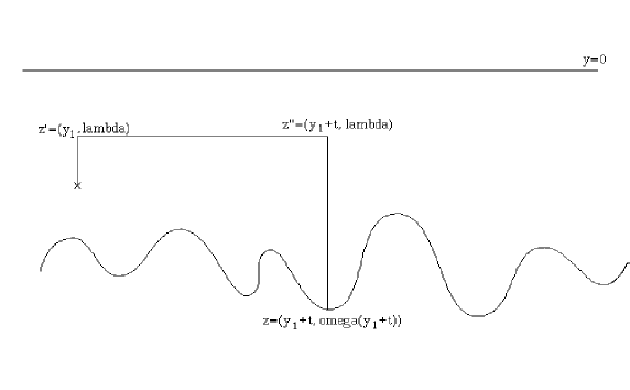
Figure 2: The path $\ell_{y,t}$.

Notice that $\ell_{y,t}$ depends in fact on $\lambda$, although the dependance is omitted in order not to burden the notation. With this choice, we have

$$\left|u(y)\cdot\nu(y_{1}+t)\right| \leq \int_{[y_{2},\lambda]}|{\partial}_{2}u|(y_{1},y_{2}^{\prime})\>dy_{2}^{\prime}$$

$$+\int_{0}^{t}|{\partial}_{1}u|(y_{1}+y_{1}^{\prime},\lambda)\>dy_{1}^{\prime}$$

$$+\int_{\omega(y_{1}+t)}^{\lambda}|{\partial}_{2}u|(y_{1}+t,y_{2}^{\prime})\>dy_{2}^{\prime}$$

$$\leq \int_{\omega(y_{1})}^{0}|{\partial}_{2}u|(y_{1},y_{2}^{\prime})\>dy_{2}^{\prime}+\int_{0}^{B}|{\partial}_{1}u|(y_{1}+y_{1}^{\prime},\lambda)\>dy_{1}^{\prime}$$

$$+\int_{\omega(y_{1}+t)}^{0}|{\partial}_{2}u|(y_{1}+t,y_{2}^{\prime})\>dy_{2}^{\prime}.$$

Integrating with respect to $y$ and $t$, we obtain, for all $\lambda\in(\sup\omega,0)$

$$\int_{y\in R}\int_{0}^{B}\left|u(y)\cdot\nu(y_{1}+t)\right|^{2}\>dy\>dt\leq C_{B}\left(\int_{R}|{\partial}_{2}u|^{2}(y)\>dy+\int_{{\mathbb{R}}}|{\partial}_{1}u|^{2}(y_{1},\lambda)\>dy_{1}\right).$$

Integrating once again with respect to $\lambda$ yields the desired inequality. ∎

$\bullet$ Let us now examine in which case assumption (2.1) is satisfied in the periodic, quasi-periodic and stationary ergodic settings: first, if $\omega$ is ${\mathbb{T}}$-periodic, where ${\mathbb{T}}:={\mathbb{R}}/{\mathbb{Z}}$, then (2.1) merely amounts to

$$\int_{{\mathbb{T}}}{\omega^{\prime}}^{2}>0.$$

Hence (H’) holds as soon as the lower boundary is not flat. In this case assumption (2.1) is necessary, as shows the following example: assume that $\omega\equiv-1$, and consider the sequence $(u_{k})_{k\geq 1}$ in $H^{1}(R)$ defined by $u_{k,2}\equiv 0$ and

$$u_{k,1}(y)=\left\{\begin{array}[]{ll}1&\text{ if }|y_{1}|\leq k,\\ 0&\text{ if }|y_{1}|\geq k+1,\end{array}\right.$$

and $u_{k,1}(y)\in[0,1]$ for all $y$, $\|\nabla u_{k,1}\|_{L^{\infty}}\leq 2.$

Then it is easily checked that $u_{k}\cdot\nu|_{\Gamma}=0,$ and that

$$\|u_{k}\|_{L^{2}(R)}\geq 2k.$$

On the other hand,

$$\|\nabla u_{k}\|_{L^{2}(R)}^{2}=\int_{k\leq y_{1}\leq k+1}|\nabla u_{k}|^{2}\leq 8\quad\forall k\geq 1.$$

Hence assumption (H’) cannot hold in $R$.

In the quasi-periodic case, the situation is similar to the one of the periodic case, i.e.

$$\eqref{hyp:nondegenerate}\iff\omega^{\prime}\neq 0.$$

Indeed, assume that

$$\omega(y_{1})=F(\lambda y_{1})$$

for some $\lambda\in{\mathbb{R}}^{d}$, $F\in\mathcal{C}^{2}({\mathbb{T}}^{d})$, with $d\geq 2$ arbitrary. Then

$$\int_{0}^{A}{\omega^{\prime}}^{2}(y_{1}+t)\>dt=\int_{0}^{A}(\lambda\cdot\nabla F)^{2}(\lambda(y_{1}+t))\>dt.$$

Write $F$ as a Fourier series:

$$F(Y)=\sum_{k\in{\mathbb{Z}}^{d}}a_{k}e^{2i\pi k\cdot Y}\quad\forall Y\in{\mathbb{T}}^{d}.$$

Then

$$\int_{0}^{A}(\lambda\cdot\nabla F)^{2}(\lambda(y_{1}+t))\>dt = -2\pi\sum_{\begin{subarray}{c}k,l\in{\mathbb{Z}}^{d},\\ \lambda\cdot(k+l)\neq 0\end{subarray}}a_{k}a_{l}\>(\lambda\cdot k)\>(\lambda\cdot l)e^{2i\pi(k+l)\cdot\lambda y_{1}}\frac{e^{2i\pi(k+l)\cdot\lambda A}-1}{i(k+l)\cdot\lambda}$$

$$+4\pi^{2}A\sum_{\begin{subarray}{c}k,l\in{\mathbb{Z}}^{d},\\ \lambda\cdot(k+l)=0\end{subarray}}a_{k}a_{l}(\lambda\cdot k)^{2}.$$

The first term is bounded uniformly in $y_{1}$ and $A$ provided the sequence $a_{k}$ is sufficiently convergent and $\lambda$ satisfies a diophantine condition. Consequently, setting

$$C_{0}=4\pi^{2}\sum_{\begin{subarray}{c}k,l\in{\mathbb{Z}}^{d},\\ \lambda\cdot(k+l)=0\end{subarray}}a_{k}a_{l}(\lambda\cdot k)^{2},$$

we deduce that there exists a constant $C$ such that

$$\forall A>0,\ \forall y_{1}\in{\mathbb{R}},\quad C_{0}A-C\leq\int_{0}^{A}{\omega^{\prime}}^{2}(y_{1}+t)\>dt\leq C_{0}A+C.$$

The above inequality entails that $C_{0}\geq 0$. If $C_{0}>0,$ inequality (2.1) is proved. If $C_{0}=0$, we infer that

$$\int_{\mathbb{R}}{\omega^{\prime}}^{2}<\infty.$$

As a consequence, since $\omega^{\prime}$ is uniformly continuous on ${\mathbb{R}}$, $\lim_{|t|\to\infty}\omega^{\prime}(t)=0$. On the other hand, it can be proved thanks to classical arguments that for all ${\varepsilon}>0,N>0$, there exists $n\in{\mathbb{N}}$ such that $n>N$ and

$$d(\lambda n,{\mathbb{Z}}^{d})\leq{\varepsilon}.$$

For ${\varepsilon}$ small and $N$ large, and $t$ in a fixed and arbitrary bounded set, we obtain

$$\omega^{\prime}(t+n) = o(1)$$

$$= \lambda\cdot{\nabla}F(\lambda t+\lambda n)$$

$$= \lambda\cdot{\nabla}F(\lambda t)+o(1)$$

$$= \omega^{\prime}(t)+o(1).$$

Thus $\omega^{\prime}(t)=0$, and $\omega^{\prime}\equiv 0$.

Hence we deduce that (2.1) is satisfied as soon as $\omega^{\prime}$ is not identically zero, at least for “generic” quasi-periodic functions (i.e. such that the Fourier coefficients of the underlying periodic function are sufficiently convergent and such that $\lambda$ satisfies a diophantine condition). In fact, slightly more refined arguments (which we leave to the reader) show that the result remains true as long as

$$\sum_{k\in{\mathbb{Z}}^{d}}|k|\;|a_{k}|<\infty,$$

without any assumption on $\lambda$.

Let us now give give another formulation of (2.1) in the stationary ergodic case. We denote by $(M,\mu)$ the underlying probability space, and by $(\tau_{y_{1}})_{y_{1}\in{\mathbb{R}}}$ the measure-preserving transformation group acting on $M$. We recall that there exists a function $F\in L^{\infty}(M)$ such that

$$\omega(y_{1},m)=F(\tau_{y_{1}}m),\quad y_{1}\in R,\ m\in M.$$

As in [6], we define the stochastic derivative of $F$ by

$${\partial}_{m}F(m):=\omega^{\prime}(0,m)\quad\forall m\in M,$$

so that $\omega^{\prime}(y_{1},m)={\partial}_{m}F(\tau_{y_{1}}m)$ for $(y_{1},m)\in{\mathbb{R}}\times M.$ We claim that almost surely in $m\in M$,

$$\inf_{y_{1}\in{\mathbb{R}}}\int_{0}^{A}|\omega^{\prime}(y_{1}+t,m)|^{2}\>dt=\mathrm{essinf}_{m^{\prime}\in M}\int_{0}^{A}|{\partial}_{m}F(\tau_{t}m^{\prime})|^{2}\>dt.$$

Indeed, notice that the left-hand side is invariant under the transformation group $(\tau_{z_{1}})_{z_{1}\in{\mathbb{R}}}$ as a function of $m\in M$. As a consequence, it is constant (almost surely) over $M$; we denote by $\phi$ the value of the constant. Since $\omega^{\prime}\in L^{\infty}$, we also have

$$\phi=\inf_{y_{1}\in{\mathbb{Q}}}\int_{0}^{A}|\omega^{\prime}(y_{1}+t,m)|^{2}\>dt\quad\text{a.s. in }M.$$

Now, for all $y_{1}\in{\mathbb{Q}}$,

$$\int_{0}^{A}|\omega^{\prime}(y_{1}+t,m)|^{2}\>dt = \int_{0}^{A}|{\partial}_{m}F(\tau_{t}(\tau_{y_{1}}m))\>dt$$

$$\geq \mathrm{essinf}_{m^{\prime}\in M}\int_{0}^{A}|{\partial}_{m}F(\tau_{t}m^{\prime})|^{2}\>dt=:\phi^{\prime}$$

almost surely in $M$. Taking the infimum over $y_{1}\in{\mathbb{Q}},$ we infer that $\phi\geq\phi^{\prime}.$

On the other hand, by definition of $\phi^{\prime}$, for all ${\varepsilon}>0$, there exists $\mathcal{M}_{\varepsilon}\subset M$ such that $P(\mathcal{M}_{\varepsilon})>0$ and

$$\phi^{\prime}\leq\int_{0}^{A}|{\partial}_{m}F(\tau_{t}m)|^{2}\>dt\leq\phi^{\prime}+{\varepsilon}\quad\forall m\in\mathcal{M}_{\varepsilon}.$$

Consequently, for all $m\in\mathcal{M}_{\varepsilon}$, we have

$$\inf_{y_{1}\in{\mathbb{R}}}\int_{0}^{A}|\omega^{\prime}(y_{1}+t,m)|^{2}\>dt\leq\int_{0}^{A}|\omega^{\prime}(t,m)|^{2}\>dt\leq\phi^{\prime}+{\varepsilon},$$

that is,

$$\phi\leq\phi^{\prime}+{\varepsilon}.$$

Hence $\phi=\phi^{\prime}.$ Eventually, we deduce that in the stationary ergodic case, assumption (2.1) is equivalent to

$$\exists A>0,\ \mathrm{essinf}_{m\in M}\int_{0}^{A}|{\partial}_{m}F(\tau_{t}m)|^{2}\>dt>0.$$ (2.4)

A straightforward application of the stationary ergodic theorem shows that (2.4) implies that

$$E[|{\partial}_{m}F|^{2}]>0.$$

However, assumption (2.4) appears to be much more stringent than the latter condition: indeed, (2.4) is a uniform condition over the probability space $M$, whereas the convergence

$$\frac{1}{R}\int_{0}^{R}|{\partial}_{m}F(\tau_{t}m)|^{2}\>dt\underset{R\to\infty}{\longrightarrow}E[|{\partial}_{m}F|^{2}]$$

only holds pointwise.

$\bullet$ Let us now compare condition (2.1) with the assumption (H) of [8]. In order to have a common ground for the comparison, we assume that the setting is stationary ergodic. In this case, the family of Young measures associated with the sequence $\omega^{\prime}(\cdot)/{\varepsilon}$ can be easily identified: indeed, according to the results of Bourgeat, Mikelic and Wright (see [7]), for all $G\in\mathcal{C}^{1}({\mathbb{R}})$ and for all test function $\varphi\in L^{1}({\mathbb{R}}\times M)$, there holds

$$\int_{{\mathbb{R}}\times M}G\left(\omega^{\prime}\left(\frac{y_{1}}{{\varepsilon}},m\right)\right)\varphi(y_{1},m)\>dy_{1}\>d\mu(m)\to\int_{{\mathbb{R}}\times M}E[G({\partial}_{m}F)]\varphi(y_{1},m)\>dy_{1}\>d\mu(m).$$

By definition of the Young measure, the left-hand side also converges (up to a subsequence) towards

$$\int_{{\mathbb{R}}\times M}\langle G,d\mu_{y_{1}}\rangle\varphi(y_{1},m))\>dy_{1}\>d\mu(m).$$

As a consequence, we obtain

$$\langle G,d\mu_{y_{1}}\rangle=E[G({\partial}_{m}F)]\quad\text{for a.e. }y_{1}\in{\mathbb{R}}.$$

Hence condition (H) is equivalent (in the stationary ergodic setting) to

$$E[|{\partial}_{m}F|^{2}]>0,\quad\text{i.e. }F\text{ non constant a.s.}$$

We deduce that assumptions (H) and (H’) are equivalent in the periodic and quasi-periodic settings. In the general stationary ergodic setting, however, condition (2.1) is stronger than (H). But since we do not know whether (2.4) is a necessary condition for (H’) in the stationary setting, we cannot really assert that (H’) is stronger than (H).

2.2 Korn-type inequalities: assumption (H”)

We now give a sufficient condition for (H”). Notice that our work in this regard is related to the paper by Desvillettes and Villani [10], in which the authors prove that for all bounded domains $\Omega\subset{\mathbb{R}}^{N}$ which lack an axis of symmetry, there exists a constant $K(\Omega)>0$ such that

$$\|D(u)\|_{L^{2}(\Omega)}\geq K(\Omega)\|\nabla u\|_{L^{2}(\Omega)}$$

$$\forall u\in H^{1}(\Omega)^{N}\ \text{s.t. }u\cdot\nu|_{{\partial}\Omega}=0.$$

The differences with our work are two-fold: first, in our case, the domain $R$ is an unbounded strip, which prevents us from using Rellich compactness results in order to prove (H”). Moreover, the tangency condition only holds on the lower boundary of $R$. However, as in [10], we show that condition (H”) is in fact related to the absence of rotational invariance of the boundary $\Gamma$. Let us stress that this notion is related, although not equivalent, to the non-degeneracy assumption of the previous paragraph (see (2.1)).

We first define the set of rotational invariant curves:

Definition 4.

For $(y_{0},R)\in{\mathbb{R}}^{2}\times[0,\infty)$, denote by $\mathcal{C}(y_{0},R)$ the circle with center $y_{0}$ and radius $R$.

For all $A>0$, we set

$$\mathcal{R}_{A} := \{\gamma\in W^{1,\infty}([0,A])^{2},\ \exists(y_{0},R)\in{\mathbb{R}}^{2}\times(0,\infty),\ \gamma([0,A])\subset\mathcal{C}(y_{0},R)\}$$

$$\cup\{\gamma\in W^{1,\infty}([0,A])^{2},\nu_{\gamma}=\text{cst.}\},$$

where $\nu_{\gamma}$ is a normal vector to the curve $\gamma$, namely

$$\nu_{\gamma}=\frac{1}{({\gamma_{1}^{\prime}}^{2}+{\gamma_{2}^{\prime}}^{2})}\begin{pmatrix}-\gamma_{2}^{\prime}\\ \gamma_{1}^{\prime}\end{pmatrix}.$$

Notice that $\mathcal{R}_{A}$ is a closed set with respect to the weak - $\ast$ topology in $W^{1,\infty}$.

We then have the following result:

Lemma 5.

Let $\omega\in W^{1,\infty}({\mathbb{R}})$. For $A>0$, $k\in{\mathbb{Z}}$, let

$$\gamma_{k}^{A}:y_{1}\in[0,A]\mapsto(y_{1},\omega(y_{1}+kA)).$$

Assume that there exists $A>0$ such that

$$\overline{\{\gamma_{k}^{A},k\in{\mathbb{Z}}\}}\cap\mathcal{R}_{A}=\emptyset,$$ (2.5)

where the closure is taken with respect to the weak - $\ast$ topology in $W^{1,\infty}.$ Then (H”) holds.

Assumption (2.5) means that each slice of length $A$ of the boundary remains bounded away from the set of curves which are invariant by rotation. In particular, in the periodic case, a simple convexity argument shows that all non-flat boundaries satisfy (2.5) (it suffices to choose $A$ equal to the period of the function $\omega$).

The proof of Lemma 5 uses the following technical result:

Lemma 6.

For all $Y>\sup\omega$, let

$$R_{Y}:=\{y\in{\mathbb{R}}^{2},\;\omega(y_{1})<y_{2}<Y\}.$$

Consider the assertion

$$(K_{Y})\quad\exists C_{Y}>0,\ \forall u\in H^{1}(R_{Y})\text{ s.t. }u\cdot\nu|_{\Gamma}=0,\ \int_{R_{Y}}|u(y)|^{2}\;dy\leq C_{Y}\int_{R_{Y}}|D(u)|^{2}.$$

If there exists $Y_{0}$ such that $(K_{Y_{0}})$ is true, then $(K_{Y})$ is true for all $Y>\sup\omega$.

We postpone the proof of Lemma 6 until the end of the section.

Let us now prove Lemma 5: the idea is to reduce the problem to the study of a Korn-like inequality in a fixed compact set, and then to use standard techniques similar to the proof of the Poincaré inequality in a bounded domain.

First step: reduction to a flat strip.

According to Lemma 6, it is sufficient to prove the result in a domain $R_{Y}$ for some $Y>\sup\omega$ sufficiently large (notice that the boundary $\Gamma$ is common to all domains $R_{Y}$).

We use the extension operator for Lipschitz domains defined by Nitsche in [20]. Since the result of Nitsche is set in a half-space over a Lipschitz curve, we recall the main ideas of the construction, and show that all arguments remain valid in the case of a strip, provided the width of the strip is large enough.

We denote by $\Omega_{-}$ the lower half-plane below $\Gamma$, namely

$$\Omega_{-}:=\{y\in{\mathbb{R}}^{2},\ y_{2}<\omega(y_{1})\}.$$

According to the results of Stein (see [22]), there exists a “generalized distance” $\delta\in\mathcal{C}^{\infty}(\Omega_{-})$ such that

$$0<2(\omega(y_{1})-y_{2})\leq\delta(y)\leq C_{0}(\omega(y_{1})-y_{2})\quad\forall y\in\Omega_{-},$$

$$|{\partial}^{\alpha}_{y}\delta(y)|\leq C_{\alpha}\delta(y)^{1-|\alpha|}\quad\forall\alpha\in{\mathbb{N}}^{2}\ \forall y\in\Omega_{-}.$$

(In general, since $\omega$ is merely a Lipschitz function, the function $d(\cdot,\Gamma)$ has very little regularity, whence the need for a generalized distance.)

Let $\psi\in\mathcal{C}([1,2])$ such that

$$\int_{1}^{2}\psi(\lambda)\>d\lambda=1,\quad\int_{1}^{2}\lambda\psi(\lambda)\>d\lambda=0.$$

For $u\in H^{1}(R_{Y})$, define an extension $\tilde{u}$ of $u$ in a strip $(\inf\omega-\eta,Y)$ for some $\eta>0$ by

$$\tilde{u}(y) = u(y)\quad\text{if }y\in R_{Y},$$

$$\tilde{u}_{i}(y): = \int_{1}^{2}\psi(\lambda)\left[u_{i}(y_{\lambda})+\lambda{\partial}_{i}\delta(y)\>u_{2}(y_{\lambda})\right]\>d\lambda,\text{ if }y\in\Omega_{-}$$

$$\text{where }y_{\lambda}:=(y_{1},y_{2}+\lambda\delta(y)),$$

Choose $Y$ such that

$$Y>2C_{0}\sup\omega-(2C_{0}-1)\inf\omega.$$

Then if $\eta>0$ is sufficiently small, $y_{\lambda}\in R_{Y}$ for all $y\in(\inf\omega-\eta,Y)$. The function $\tilde{u}$ thus defined does not have any jump across $\Gamma$. Moreover, it can be checked that

$$\|D(\tilde{u})\|_{L^{2}({\mathbb{R}}\times(\inf\omega-\eta,Y))}\leq C\|D(u)\|_{L^{2}(R)}.$$

Indeed, if $y\in\Omega_{-}$ and $y_{2}>\inf\omega-\eta$,

$$\left[{\partial}_{i}\tilde{u}_{j}+{\partial}_{j}\tilde{u}_{i}\right](y) = \int_{1}^{2}d\lambda\psi(\lambda)\left[\left({\partial}_{i}u_{j}+{\partial}_{j}u_{i}\right)(y_{\lambda})+2\lambda^{2}{\partial}_{i}\delta(y){\partial}_{j}\delta(y){\partial}_{2}u_{2}(y_{\lambda})\right.$$

$$\qquad\qquad\qquad+\lambda{\partial}_{i}\delta(y)\left({\partial}_{2}u_{j}+{\partial}_{j}u_{2}\right)(y_{\lambda})$$

$$\qquad\qquad\qquad+\lambda{\partial}_{j}\delta(y)\left({\partial}_{2}u_{i}+{\partial}_{i}u_{2}\right)(y_{\lambda})$$

$$\qquad\qquad\qquad\left.+2\lambda{\partial}^{2}_{ij}\delta(y)u_{2}(y_{\lambda})\right].$$

Writing $u_{2}(y_{\lambda})$ as

$$u_{2}(y_{\lambda})=u_{2}(y_{1},y_{2}+\delta(y))+\int_{1}^{\lambda}{\partial}_{2}u_{2}(y_{\mu})\>d\mu$$

and using the condition $\int_{1}^{2}\lambda\psi(\lambda)\>d\lambda=0$ yields

$$|D(\tilde{u})(y)|\leq C\int_{1}^{2}|D(u)|(y_{\lambda})\>d\lambda.$$

A careful analysis of the right-hand side then allows to prove that

$$\int_{\mathbb{R}}dy_{1}\int_{\inf\omega-\eta}^{\omega(y_{1})}dy_{2}|D(\tilde{u})(y)|^{2}\leq C\int_{R_{Y}}|D(u)|^{2}.$$

For all additional details, we refer to [20].

Consequently, we have built an extension operator

$$E:H^{1}(R_{Y})\mapsto H^{1}({\mathbb{R}}\times(\inf\omega-\eta,Y))$$

such that for all $u\in H^{1}(R_{Y})$,

$$\|D(u)\|_{L^{2}(R_{Y})}\leq\|D(Eu)\|_{L^{2}({\mathbb{R}}\times(\inf\omega-\eta))}\leq C\|D(u)\|_{L^{2}(R_{Y})},$$

$$\|u\|_{L^{2}(R_{Y})}\leq\|Eu\|_{L^{2}({\mathbb{R}}\times(\inf\omega-\eta))}\leq C\|u\|_{L^{2}(R_{Y})}.$$

Second step: compactification of the problem.

In the rest of the proof, we set $Q:={\mathbb{R}}\times(\inf\omega-\eta,Y)$. According to the first step, we now have to prove the existence of a constant $C$ such that for any function $u\in H^{1}(Q)$ satisfying $u\cdot\nu|_{\Gamma}=0$,

$$\|u\|_{L^{2}(Q)}\leq C\|D(u)\|_{L^{2}(Q)}.$$

Of course, it is sufficient to prove that there exists a constant $C_{A}$ such that for all $k\in{\mathbb{Z}}$,

$$\|u\|_{L^{2}(Q_{k,A})}\leq C_{A}\|D(u)\|_{L^{2}(Q_{k,A})}\quad\forall u\in H^{1}(Q_{k,A})\text{ s.t. }u\cdot\nu|_{\Gamma_{k}^{A}}=0$$ (2.6)

where

$$Q_{k,A}=Q\cap\{y,\>kA<y_{1}<(k+1)A\}.$$

Assume by contradiction that (2.6) is false. Then there exists a sequence of relative integers $(k_{n})_{n\geq 1}$ and a sequence $u_{n}\in H^{1}(Q_{k_{n},A})$, such that for all $n$,

$$\|u_{n}\|_{L^{2}(Q_{k_{n},A})}\geq n\|D(u_{n})\|_{L^{2}(Q_{k_{n},A})}.$$

In the rest of the proof, we drop all sub- and superscripts $A$ in $Q_{k,A}$, $\gamma_{k}^{A}$ in order to lighten the notation.

Let $v_{n}:=u_{n}(\cdot+(k_{n},0))/\|u_{n}\|_{L^{2}}$. Then $v_{n}\in H^{1}(Q_{0})$ for all $n$ and

$$v_{n}\cdot\nu|_{\Gamma_{k_{n}}}=0,\quad\|v_{n}\|_{L^{2}(Q_{0})}=1,\ \|D(v_{n})\|_{L^{2}(Q_{0})}\leq\frac{1}{n}.$$

According to the standard Korn inequality (see for instance [20]), there exists $C>0$ such that for all $v\in H^{1}(Q_{0})$,

$$\|\nabla v\|_{L^{2}(Q_{0})}\leq C(\|v\|_{L^{2}(Q_{0})}+\|D(v)\|_{L^{2}(Q_{0})}).$$

As a consequence, the sequence $v_{n}$ is bounded in $H^{1}(Q_{0})$. By Rellich compactness, there exists a subsequence (still denoted by $v_{n}$) and a limit function $\bar{v}\in H^{1}(Q_{0})$ such that

$$v_{n}\rightharpoonup\bar{v}\quad\text{in }w-H^{1}(Q_{0}),$$

$$v_{n}\to\bar{v}\quad\text{in }L^{2}(Q_{0}).$$

We deduce that $D(\bar{v})=0$ and $\|\bar{v}\|_{L^{2}}=1$. Hence $\bar{v}$ is a non-zero solid vector field: there exists $(C,y_{0})\in({\mathbb{R}}\times{\mathbb{R}}^{2})\setminus\{0\}$ such that

$$\bar{v}(y)=(Cy+y_{0})^{\bot}\quad\text{for a.e. }y\in Q_{0}.$$

On the other hand, for all $n\in{\mathbb{N}}$, for almost every $y_{1}\in[0,A]$, we have

$$v_{n,1}(\gamma_{k_{n}}(y_{1}))\gamma_{k_{n},2}^{\prime}(y_{1})-v_{n,2}(\gamma_{k_{n}}(y_{1}))\ \gamma_{k_{n},1}^{\prime}(y_{1})=0.$$ (2.7)

Since the sequence $\gamma_{k_{n}}$ is bounded in $W^{1,\infty}$, up to the extraction of a further subsequence, $\gamma_{k_{n}}$ converges weakly - $\ast$ in $W^{1,\infty}$ towards a function $\bar{\gamma}$. Since $\gamma_{k_{n},1}(y_{1})=y_{1}$ for all $n$, we deduce that $(\gamma_{k_{n}}-\bar{\gamma})\cdot e_{1}=0$. We then pass to the limit in the identity (2.7) using the following facts:

• $\gamma_{k_{n}}\to\bar{\gamma}$ in $L^{\infty}$, and thus

  $$\int_{0}^{A}\left|v_{n}(\gamma_{k_{n}})-v_{n}(\bar{\gamma})\right|^{2}\leq C\|\gamma_{k_{n}}-\bar{\gamma}\|_{\infty}\|\nabla v_{n}\|_{L^{2}}^{2}\to 0;$$

• $v_{n}(\bar{\gamma})$ is bounded in $H^{1/2}((0,A))$, and thus

  $$v_{n}(\bar{\gamma})\to\bar{v}(\bar{\gamma})\quad\text{in }L^{2}(0,A).$$

At the limit, we obtain

$$(C\bar{\gamma}+y_{0})\cdot\bar{\gamma}^{\prime}=0,$$

i.e.

$$|C\bar{\gamma}+y_{0}|^{2}=\text{cst.}$$

We deduce that $\bar{\gamma}\in\mathcal{R}_{A}$, and thus $\mathcal{R}_{A}\cap\overline{\{\gamma_{k},k\in{\mathbb{Z}}\}}\neq\emptyset$, which contradicts the assumption of the lemma. Thus (2.6) holds, which completes the proof.∎

Remark 7.

• We emphasize that condition (2.5) is probably not optimal. Indeed, (2.5) amounts to requiring that the inequality

  $$\|u\|_{L^{2}}\leq C\|D(u)\|_{L^{2}}$$

  holds uniformly in each slice of length $A$. However, since our proof relies on compactness results in $L^{2}$, it seems necessary to work in a fixed compact domain. Of course, if a more “constructive” proof were at hand (in the spirit of Lemma 3), it is likely that (2.5) could be weakened.

• We have already pointed out that in the periodic case, conditions (2.5) and (2.1) are equivalent. In the general case, however, (2.5) is stronger than (2.1). Indeed, (2.1) merely requires the frontier $\Gamma$ to be non-flat (uniformly on $R$), whereas (2.1) requires that is not invariant by rotation, in addition to being non-flat.

• We have used in the proof the following Korn inequality: since the function $\omega$ is Lipschitz continuous, there exists a constant $C_{K}>0$ such that

  $$\|u\|_{H^{1}(R)}\leq C_{K}(\|u\|_{L^{2}(R)}+\|D(u)\|_{L^{2}(R)})\quad\forall u\in H^{1}(R).$$

  We refer to [20] (see also [11]) for a proof. The constant $C_{K}$ depends only on the Lipschitz constant of $\omega$. The inequality holds without any assumption on the non-degeneracy of the boundary or on the behaviour of $u$ at the boundary $\Gamma$.

We now prove Lemma 6. Assume that there exists $Y_{0}$ such that $(K_{Y_{0}})$ holds true. Let us first prove that $(K_{Y})$ is true for all $Y\in(\sup\omega,Y_{0})$. Let $u\in H^{1}(R_{Y})$ be arbitrary. Using a construction similar to the one of Nitsche (see [20]), we define an extension $u_{1}\in H^{1}(R_{Y_{1}})$ of $u$ such that

$$Y_{1}=\sup\omega+2(Y-\sup\omega),$$

$$\|u_{1}\|_{L^{2}(R_{Y_{1}})}\leq C_{1}\|u\|_{L^{2}(R_{Y})},\quad\|D(u_{1})\|_{L^{2}(R_{Y_{1}})}\leq C_{1}\|D(u)\|_{L^{2}(R_{Y})}.$$

Iterating this process, we define sequences $(Y_{n})_{n\geq 0},(u_{n})_{n\geq 0}$ such that $u_{n}\in H^{1}(R_{Y_{n}})$ and $u_{n+1}$ is an extension of $u_{n}$ for all $n$, and

$$Y_{n+1}=\sup\omega+2(Y_{n}-\sup\omega),$$

$$\|u_{n+1}\|_{L^{2}(R_{Y_{n+1}})}\leq C_{n+1}\|u_{n}\|_{L^{2}(R_{Y_{n}})},\quad\|D(u_{n+1})\|_{L^{2}(R_{Y_{n+1}})}\leq C_{n+1}\|D(u_{n})\|_{L^{2}(R_{Y_{n}})}.$$

It can be easily checked that $\lim_{n\to\infty}Y_{n}=\infty$, and thus there exists $n_{0}>0$ such that $Y_{n_{0}}>Y_{0}$. By construction, $u_{n_{0}}\in H^{1}(R_{Y_{0}})$ and there exists a constant $C$ such that

$$\|u_{n_{0}}\|_{L^{2}(R_{Y_{n_{0}}})}\leq C\|u\|_{L^{2}(R_{Y})},\quad\|D(u_{n_{0}})\|_{L^{2}(R_{Y_{n_{0}}})}\leq C\|D(u)\|_{L^{2}(R_{Y})}.$$

Moreover,

$$u=u_{n_{0}}\quad\text{on }R_{Y}.$$

$\vartriangleright$ From $(K_{Y_{0}})$, we infer that

$$\|u_{n_{0}}\|_{L^{2}(R_{Y_{0}})}\leq C_{Y_{0}}\|D(u_{n_{0}})\|_{L^{2}(R_{Y_{0}})},$$

and thus

$$\|u\|_{L^{2}(R_{Y})}\leq C\|D(u)\|_{L^{2}(R_{Y})}.$$

Hence $(K_{Y})$ is satisfied.

Let us now prove that $(K_{Y})$ is also true for all $Y>Y_{0}$. Let $u\in H^{1}(R_{Y})$ arbitrary; then $u\in H^{1}(R_{Y_{0}})$, and

$$\|u\|_{L^{2}(R_{Y_{0}})}\leq C_{Y_{0}}\|D(u)\|_{L^{2}(R_{Y_{0}})}.$$

Moreover, according to the classical Korn inequality in the channel $R_{Y_{0}}$, there exists a constant $C_{K}$ such that

$$\|u\|_{H^{1}(R_{Y_{0}})}\leq C_{K}\left(\|u\|_{L^{2}(R_{Y_{0}})}+\|D(u)\|_{L^{2}(R_{Y_{0}})}\right).$$

Let $\Sigma:={\mathbb{R}}\times\{Y_{0}\}$. Then

$$\|u\|_{L^{2}(\Sigma)}\leq C\|u\|_{H^{1}(R_{Y_{0}})}\leq C\|D(u)\|_{L^{2}(R_{Y_{0}})}.$$

Now, for any $y\in{\mathbb{R}}\times(Y_{0},Y)$, let $y^{\prime}\in\Sigma$ such that

$$y^{\prime}=y+t(1,-1)\quad\text{for some }t\in{\mathbb{R}}.$$

Then

$$u(y)=u(y^{\prime})+t\int_{0}^{1}({\partial}_{1}-{\partial}_{2})u(y+t(1-\tau)(1,-1))d\tau.$$

Notice that

$$(1,-1)\cdot({\partial}_{1}-{\partial}_{2})u={\partial}_{1}u_{1}+{\partial}_{2}u_{2}-({\partial}_{1}u_{2}+{\partial}_{2}u_{1}),$$

and thus

$$\int_{\mathbb{R}}\int^{Y}_{Y_{0}}\left|u(y)\cdot(1,-1)\right|^{2}\>dy \leq C\left(\|u\|_{L^{2}(\Sigma)}^{2}+\int_{\mathbb{R}}\int^{Y}_{Y_{0}}\left|D(u)\right|^{2}\right)$$

$$\leq C\|Du\|^{2}_{L^{2}(R_{Y})}.$$

Similarly,

$$\int_{\mathbb{R}}\int_{Y}^{Y_{0}}\left|u(y)\cdot(-1,-1)\right|^{2}\>dy\leq C\|D(u)\|^{2}_{L^{2}(R_{Y})}.$$

Eventually, we obtain

$$\|u\|_{L^{2}(R_{Y})}\leq C\|Du\|^{2}_{L^{2}(R_{Y})},$$

which completes the proof.

3 Estimates for the no-slip condition

In this section, we will prove Theorem 1. In other words, we will establish, for any sequence $\lambda^{\varepsilon}\in[0,+\infty]$, the well-posedness result and the error estimates that were established in [6] for $\lambda^{\varepsilon}=0$. We will use the same general strategy, based on the work of Ladyzenskaya and Solonnikov [17]. However, the handling of the slip type conditions will require new arguments, due to a loss of control on the skew-symmmetric part of the gradient. Moreover, we shall specify the dependence of the error terms with respect to $\phi$. We shall of course put the stress on these new arguments.

The starting point of the proof is an approximation scheme by solutions in truncated channels. Therefore,we introduce the notations

$$\forall\,k,l\geq 0,\quad U_{k,l}\>:=\>U\cap\{k<|x_{1}|<l\},\quad U_{k}\>:=\>U_{-k,k},$$

for any set $U$ of ${\mathbb{R}}^{2}$. We take as a new unknown

$$v\>:=\>u^{\varepsilon}-\tilde{u}^{0},\quad\tilde{u}^{0}\>:=\>1_{\Omega}\,u^{0}$$

where $u^{0}$ is the Poiseuille flow. As a new pressure, we take

$$q\>:=\>p\>+\>12\phi x_{1}.$$

It formally satisfies

$$\left\{\begin{aligned} -\Delta v+\tilde{u}^{0}\cdot{\nabla}v+v\cdot{\nabla}\tilde{u}^{0}+v\cdot{\nabla}v+{\nabla}q&\>=\>1_{R^{\varepsilon}}(-12\phi,0),\>x\in\Omega^{\varepsilon},\\ \hbox{div }v&\>=\>0,\>x\in\Omega^{\varepsilon},\\ v|_{x_{2}=1}\>=\>0,\>\int_{\sigma^{\varepsilon}}v_{1}&\>=\>0,\\ v_{\tau}|_{\Gamma^{\varepsilon}}\>=\>\lambda^{\varepsilon}&(D(v)\nu)_{\tau}|_{\Gamma^{\varepsilon}},\quad v\cdot\nu|_{\Gamma^{\varepsilon}}\>=\>0,\end{aligned}\right.$$ (3.1)

where $\nu$ is the inward pointing normal vector on $\Gamma^{\varepsilon}$ and

$$v_{\tau}=(I_{d}-\nu\otimes\nu)v$$

denotes the tangential part of $v$ on $\Gamma^{\varepsilon}$. The system is supplemented with the following jump conditions at the interface $\Sigma$:

$$[v]|_{\Sigma}=0,\quad[-D(v)e_{2}+qe_{2}]|_{\Sigma}=(-6\phi,0).$$

In order to build and estimate the field $v$, we consider the approximate problems in $\Omega^{\varepsilon}_{n}$

$$\left\{\begin{aligned} -\Delta v+\tilde{u}^{0}\cdot{\nabla}v+v\cdot{\nabla}\tilde{u}^{0}+v\cdot{\nabla}v+{\nabla}q&\>=\>1_{R^{\varepsilon}}(12\phi,0),\>x\in\Omega^{\varepsilon}_{n},\\ \hbox{div }v&\>=\>0,\>x\in\Omega_{n}^{\varepsilon},\\ v|_{x_{1}=n}\>=\>v|_{x_{1}=-n}\>=\>v|_{x_{2}=1}&\>=\>0,\\ v_{\tau}|_{\Gamma^{\varepsilon}_{n}}\>=\>\lambda^{\varepsilon}&(D(v)\nu)_{\tau}|_{\Gamma^{\varepsilon}_{n}},\quad v\cdot\nu|_{\Gamma^{\varepsilon}_{n}}\>=\>0,\end{aligned}\right.$$ (3.2)

and

$$[v]|_{\Sigma_{n}}\>=\>0,\quad[-D(v)e_{2}+qe_{2}]|_{\Sigma_{n}}\>=\>(-6\phi,0).$$

The proof divides into four steps:

1. We construct a solution $v_{n}\>$ of the approximate system (3.2).

2. We derive $H^{1}_{uloc}$ estimates on $v_{n}$ that are uniform in $n$. This yields compactness of $(v_{n})_{n}$, hence, as $n$ goes to infinity, a solution $u$ of (NS^ε).

3. We prove uniqueness of this solution $u$.

4. We deduce from the previous steps the desired $O(\sqrt{{\varepsilon}})$ bound in $H^{1}_{uloc}$ for $u-u^{0}$. From there, using duality arguments, we get the $O({\varepsilon})$ bound in $L^{2}_{uloc}$.

Step 1. The wellposedness of (3.2) relies on an a priori estimate over $\Omega^{\varepsilon}_{n}$. Multiplying formally by $v$, we obtain

$$\int_{\Omega^{\varepsilon}_{n}}|D(v)|^{2}\>+\>(\lambda^{\varepsilon})^{-1}\int_{\Gamma^{\varepsilon}_{n}}|v_{\tau}|^{2}\>=\>-\int_{\Omega_{n}^{\varepsilon}}\left(\tilde{u}^{0}\otimes v+v\otimes\tilde{u}^{0}\right):D(v)-\int_{R^{\varepsilon}_{n}}12\phi\,v_{1}+\int_{\Sigma^{\varepsilon}_{n}}6\phi v_{1},$$

where $v_{\tau}$ denotes the tangential part of $v$. As $\|{\nabla}u^{0}\|_{\infty}\>\leq\>C\,\phi$, we obtain

$$\|D(v)\|_{L^{2}(\Omega^{\varepsilon}_{n})}^{2}\>\leq\>C\,\phi\,\left(\|v\|_{L^{2}(\Omega^{\varepsilon}_{n})}\,\|D(v)\|_{L^{2}(\Omega^{\varepsilon}_{n})}\>+\>\sqrt{n\,{\varepsilon}}\,\|v\|_{L^{2}(R^{\varepsilon}_{n})}\>+\>\sqrt{n}\,\|v\|_{L^{2}(\Sigma^{\varepsilon}_{n})}\right).$$ (3.3)

As $v$ is zero at the upper boundary of the channel, Poincaré inequality applies, to provide

$$\|v\|_{L^{2}(\Omega^{\varepsilon}_{n})}\>\leq\>C\,\|{\nabla}v\|_{L^{2}(\Omega^{\varepsilon}_{n})}.$$

where $C$ depends only on the height of the channel. Let

$$\Omega^{\varepsilon}_{bl}\>:=\>\{x,\>x_{2}>{\varepsilon}\omega(x_{1}/{\varepsilon})\}$$

the “rough” half plane, and $\tilde{v}\in H^{1}(\Omega^{\varepsilon}_{bl})$ the extension of $v$ which is zero outside $\Omega^{\varepsilon}_{n}$. We can apply to $\tilde{v}$ the results of Nitsche [20] on the Korn inequality in a half plane bounded by a Lipschitz curve: one has

$$\|{\nabla}\tilde{v}\|_{L^{2}(\Omega^{\varepsilon}_{bl})}\>\leq\>{\cal C}\,\|D(\tilde{v})\|_{L^{2}(\Omega^{\varepsilon}_{bl})}$$

where the constant ${\cal C}$ only depends on the Lipschitz constant of the curve. For $\Omega^{\varepsilon}_{bl}$, this Lipschitz constant, and therefore the estimates, are uniform in ${\varepsilon}$. We insist that this inequality is homogenenous: it does not involve the $L^{2}$ norm of $\tilde{v}$, contrary to the more general inhomogeneous Korn inequality. Back to $v$, we get

$$\|{\nabla}v\|_{L^{2}(\Omega^{\varepsilon}_{n})}\>\leq\>C\|D(v)\|_{L^{2}(\Omega^{\varepsilon}_{n})}.$$

Hence, denoting for all $k\in{\mathbb{N}}$

$$E_{k}\>:=\>\|v\|^{2}_{L^{2}(\Omega^{\varepsilon}_{k})}\>+\>\|{\nabla}v\|^{2}_{L^{2}(\Omega^{\varepsilon}_{k})}\>+\>\|D(v)\|^{2}_{L^{2}(\Omega^{\varepsilon}_{k})}$$

the combination of Poincaré and Korn inequalities leads to $E_{n}\>\leq\>C\|D(v)\|^{2}_{L^{2}(\Omega^{\varepsilon}_{n})}$.

Now, by rescaling either the Poincaré inequality when $\lambda^{\varepsilon}=0$, or the inequality in (H’) when $\lambda^{\varepsilon}\neq 0$, we get

$$\|v\|_{L^{2}(R^{\varepsilon}_{n})}\>\leq\>C\,{\varepsilon}\,\|{\nabla}v\|_{L^{2}(R^{\varepsilon}_{n})}.$$

Then, we deduce

$$\|v\|_{L^{2}(\Sigma^{\varepsilon}_{n})}\>\leq\>C\,\sqrt{{\varepsilon}}\,\|v\|_{H^{1}(R^{\varepsilon}_{n})}\>\leq\>C^{\prime}\,\sqrt{{\varepsilon}}\,\|{\nabla}v\|_{L^{2}(R^{\varepsilon}_{n})}.$$

Back to the energy estimate (3.3), we end up with

$$E_{n} \leq\>C\,\|D(v)\|^{2}_{L^{2}(\Omega^{\varepsilon}_{n})}\>\leq\>C^{\prime}\,\phi\left(\|v\|_{L^{2}(\Omega^{\varepsilon}_{n})}\,\|D(v)\|_{L^{2}(\Omega^{\varepsilon}_{n})}\>+\>\sqrt{n\,{\varepsilon}}\,\|{\nabla}v\|_{L^{2}(R^{\varepsilon}_{n})}\right)$$

$$\leq\>C^{\prime}\phi\left(E_{n}\>+\>\sqrt{n\,{\varepsilon}}\,\sqrt{E_{n}}\right)\>\leq\>C^{\prime}\phi E_{n}\>+\>\frac{1}{2}E_{n}\>+\>\frac{C^{\prime 2}}{2}\,\phi^{2}\,n\,{\varepsilon}.$$

so that, for $\phi$ small enough, we have the global estimate

$$E_{n}\>\leq\>C\,\phi^{2}\,n\,{\varepsilon}.$$ (3.4)

Thanks to this estimate, one obtains by classical arguments a variational solution $v_{n}\in H^{1}(\Omega^{\varepsilon}_{n})$ of (3.2). The uniqueness of this solution (for $\phi$ small enough) is deduced from the same kind of energy estimates, performed on the difference of two solutions. We leave the details to the reader.

Step 2. The next step in the proof of Theorem 1 is the derivation of uniform $H^{1}_{uloc}$ bounds on $v_{n}$. The idea, which originates in a work of Ladyzenskaya and Solonnikov, is to prove by induction on $k^{\prime}=n-k$ that

$$E_{k}\>\leq\>C_{0}\,\phi^{2}\,(k+1)\,{\varepsilon},\quad C\mbox{ large enough}.$$ (3.5)

Once the bound on the $E_{k}$’s is proved, we can use it with $k=n-1$, so that $E_{1}\>\leq\>C\,\phi^{2}{\varepsilon}$. This gives a control on a unit slice of the channel around $x_{1}=0$. But as will be clear from the proof of the induction relation, $x_{1}=0$ plays no special role: in other words the same bound holds for any unit slice of the channel, which gives the uniform $H^{1}_{uloc}$ bound.

Let us now describe the induction process. First, by (3.4), the induction assumption holds with $k^{\prime}=0$. To go from $k^{\prime}-1$ to $k^{\prime}$, that is from $k+1$ to $k$, we shall need the following inequality:

$$\forall k\leq n,\quad E_{k}\>\leq\>C_{1}\left(E_{k+1}-E_{k}\>+\>(E_{k+1}-E_{k})^{3/2}\>+\>\phi^{2}\,(k+1)\,{\varepsilon}\right).$$ (3.6)

This inequality at hand, and assuming $E_{k+1}\>\leq\>C_{0}\,\phi^{2}\,(k+2)\,{\varepsilon}$, one obtains straightforwardly that $E_{k}\>\leq\>C_{0}\,\phi^{2}\,(k+1)\,{\varepsilon}\>$ for all $k\geq C_{0}-1$ provided $C_{0}$ is chosen large enough. For $k\leq C_{0}-1$, we have merely $E_{k}\leq C_{0}\,\phi^{2}\,(\lfloor C_{0}\rfloor+1)\,{\varepsilon}\>$. Hence, up to a new definition of the constant $C_{0}$, we obtain inequality (3.5).

An inequality similar to (3.6) has been established by one of the authors in [6], for the case $\lambda^{\varepsilon}=0$. The discrete variable $k$ is replaced in [6] by a continuous variable $\eta$, but the correspondence from one to another is obvious. We also refer to the original paper [17], and to the boundary layer analysis in [13], in which similar inequalities are derived.

Relation (3.6) follows from localized energy estimates. We introduce some truncation function $\chi_{k}=\chi_{k}(x_{1})$, such that $\chi_{k}=1$ over $\Omega^{\varepsilon}_{k}$, $\chi_{k}=0$ outside $\Omega^{\varepsilon}_{k+1}$, and $|\chi^{\prime}_{k}|\leq 2$. Multiplying by $\chi_{k}\,v$ within (3.2) and integrating by parts, we deduce that

$$\int_{\Omega^{\varepsilon}}\chi_{k}|D(v)|^{2}\>+\>(\lambda^{\varepsilon})^{-1}\int_{\Gamma^{\varepsilon}}\chi_{k}|v_{\tau}|^{2}$$

$$\>\leq\> \int_{\Omega^{\varepsilon}}\chi_{k}(\tilde{u}^{0}\otimes v+v\otimes\tilde{u}^{0}):D(v)\>-\>\int_{R^{\varepsilon}}12\phi\chi_{k}v_{1}\>+\>\int_{\Sigma^{\varepsilon}}6\phi v_{1}\chi_{k}$$

$$\>+\int_{\Omega^{\varepsilon}}D(v):({\nabla}\chi_{k}\otimes v)\>+\>\int_{\Omega^{\varepsilon}}(\tilde{u}^{0}\otimes v+v\otimes\tilde{u}^{0}):({\nabla}\chi_{k}\otimes v)$$

$$\>+\>\int_{\Omega^{\varepsilon}}(v\otimes v):({\nabla}\chi_{k}\otimes v)\>+\>\int_{\Omega^{\varepsilon}}q{\nabla}\chi_{k}\cdot v\>=\>\sum_{j=1}^{7}I_{j}.$$

where ${\nabla}\chi_{k}=(\chi^{\prime}_{k},0)$. The r.h.s. of the inequality has two different parts:

• The first three terms are very similar to those of step 1. They are treated along the same lines:

  $$\sum_{j=1}^{3}|I_{j}|\>\leq\>C\,\phi\,\left(E_{k+1}+\sqrt{(k+1)\>{\varepsilon}}\,\sqrt{E_{k+1}}\right).$$

• The remaining terms involve derivatives of $\chi_{k}$: they are supported in $\Omega_{k,k+1}$. Standard manipulations yield the bounds:

  $$|I_{4}|\>+\>|I_{5}|\>\leq\>C\,(E_{k+1}-E_{k}),\quad|I_{6}|\>\leq\>C(E_{k+1}-E_{k})^{3/2}.$$

• The treatment of the pressure term is a little more tricky. We decompose

  $$\Omega^{\varepsilon}_{k,k+1}\>=\>\Omega_{k,k+1}^{{\varepsilon},-}\>\cup\>\Omega_{k,k+1}^{{\varepsilon},+},\quad\Omega_{k,k+1}^{{\varepsilon},\pm}\>:=\>\Omega^{\varepsilon}_{k,k+1}\cap\{\pm x_{1}\geq 0\}.$$

  The zero flux condition on $v$ implies that $\int_{\Omega_{k,k+1}^{{\varepsilon},\pm}}f(x_{1})v_{1}=0$ for any function $f$ depending only on $x_{1}$. Thus,

  $$I_{7}\>=\>\int_{\Omega^{\varepsilon}_{k,k+1}}q\,\chi^{\prime}_{k}\,v_{1}\>=\>\>=\>\int_{\Omega^{{\varepsilon},-}_{k,k+1}}(q-q_{k}^{-})\,\chi^{\prime}_{k}\,v_{1}\>+\>\int_{\Omega^{{\varepsilon},+}_{k,k+1}}(q-q_{k}^{+})\,\chi^{\prime}_{k}v_{1},$$

  where $q_{k}^{\pm}$ is the average of $q$ over $\Omega_{k,k+1}^{{\varepsilon},\pm}$. Then, we use the well-known estimate

  $$\left\|q-\oint_{{\cal O}}q\right\|_{L^{2}({\cal O})}\>\leq\>{\cal C}\,\|\Delta v+f\|_{H^{-1}({\cal O})}$$

  for the Stokes system

  $$-\Delta v+{\nabla}q=f,\quad\hbox{div }u=0\mbox{ in }{\cal O}$$

  where $C$ only depends on the measure of ${\cal O}$ and the Lipschitz constant of ${\partial}{\cal O}$. We take here $\displaystyle{\cal O}=\Omega_{k,k+1}^{{\varepsilon},\pm}$ (so that the constant is uniform in $k$ and ${\varepsilon}$), and

  $$f\>:=\>-\hbox{div }\left(\tilde{u}^{0}\otimes v+v\otimes\tilde{u}^{0}+v\otimes v\right)+1_{R^{\varepsilon}}(12\phi,0).$$

  From there, one gets after a few computations

  $$|I_{7}|\> \leq\>C\,\left(\|q-q_{k}^{-}\|_{L^{2}(\Omega^{{\varepsilon},-}_{k,k+1})}+\|q-q_{k}^{+}\|_{L^{2}(\Omega^{{\varepsilon},+}_{k,k+1})}\right)\,\|v\|_{L^{2}(\Omega_{k,k+1})}$$

  $$\leq\>C\,\left(\phi\,\sqrt{\,{\varepsilon}}\,\sqrt{E_{k+1}-E_{k}}\>+\>(E_{k+1}-E_{k})\>+\>(E_{k+1}-E_{k})^{3/2}\right)$$

  $$\leq\>C\,\left(\phi^{2}\,{\varepsilon}\>+\>(E_{k+1}-E_{k})\>+\>(E_{k+1}-E_{k})^{3/2}\right).$$

We refer to [6] for more details. By gathering all the inequalitites on the $I_{j}$’s, we obtain for $\phi$ small enough

$$\int_{\Omega^{\varepsilon}}\chi_{k}|D(v)|^{2} \leq C\left(E_{k+1}-E_{k}\>+\>(E_{k+1}-E_{k})^{3/2}\>+\>\phi^{2}\,(k+1)\,{\varepsilon}\right)$$ (3.8)

$$+C\phi\,\left(E_{k}+\phi\sqrt{(k+1){\varepsilon}}\sqrt{E_{k}}\right)$$

Now, we have

$$\int_{\Omega^{\varepsilon}}\chi_{k}|D(v)|^{2}\> \geq\>\int_{\Omega^{\varepsilon}}\chi_{k}^{2}|D(v)|^{2}\>\geq\>\int_{\Omega^{\varepsilon}}|D(\chi_{k}v)|^{2}\>-\>\int_{\Omega^{\varepsilon}}|\chi^{\prime}_{k}|^{2}|v^{2}|$$

$$\geq\>\int_{\Omega^{\varepsilon}}|D(\chi_{k}v)|^{2}-4(E_{k+1}-E_{k}).$$

As $\chi_{k}\,v$ is zero outside $\Omega^{\varepsilon}_{k+1}$, we can proceed as in Step 1, to get

$$\int_{\Omega^{\varepsilon}}|D(\chi_{k}v)|^{2}\>\geq\>c\,E_{k+1}\>\geq\>c\,E_{k}+c\,(E_{k+1}-E_{k}).$$

Finally,

$$\int_{\Omega^{\varepsilon}}\chi_{k}|D(v)|^{2}\>\geq\>C\,E_{k}\>-\>c\,(E_{k+1}-E_{k}).$$

Combining this inequality with (3.8) gives the result provided $\phi$ is small enough.

As we have already explained, once inequality (3.6) is proved, one obtains easily a $O(\sqrt{{\varepsilon}})$ $\,H^{1}_{uloc}$ bound on $v_{n}$. By standard compactness arguments, any accumulation point $v$ of $(v_{n})$ is a solution of (3.1). It provides a solution $u^{\varepsilon}$ of the original system (NS^ε). Moreover,

$$\|u^{\varepsilon}-u^{0}\|_{H^{1}_{uloc}(\Omega^{\varepsilon})}\>\leq\>C\,\phi\,\sqrt{{\varepsilon}},\quad\|u^{\varepsilon}\|_{H^{1}_{uloc}(\Omega^{\varepsilon})}\>\leq\>C\,\phi.$$ (3.9)

Step 3. It remains to prove the uniqueness of the solution in $H^{1}_{uloc}$.

Let now $v=u^{{\varepsilon},2}-u^{{\varepsilon},1}$ the difference between two solutions of (NS^ε). It satisfies

$$-\Delta v+\hbox{div }\left(u^{{\varepsilon},1}\otimes v+v\otimes u^{{\varepsilon},1}+v\otimes v\right)+{\nabla}q=0$$

together with $\hbox{div }v=0$ and homogeneous jump and boundary conditions. We can always assume that $u^{{\varepsilon},1}$ satisfies the bounds in (3.9). Then, performing energy estimates similar to those of Step 2, we get, for $\phi$ small enough:

$$\forall k,\>\quad E_{k}\>\leq\>C\left((E_{k+1}-E_{k})\>+\>(E_{k+1}-E_{k})^{3/2}+\>\phi\,\sqrt{{\varepsilon}}\,E_{k}\right)$$

We have used implicitly that

$$\left|\int_{\Omega^{\varepsilon}}\chi_{k}u^{{\varepsilon},1}\otimes\,v:{\nabla}(v)\right|\> \leq\>\sum_{j=0}^{k}\int_{\Omega^{\varepsilon}_{j,j+1}}|u^{{\varepsilon},1}|\,|v|\,|{\nabla}(v)|$$

$$\leq\>\sum_{j=0}^{k}\|u^{{\varepsilon},1}\|_{L^{4}(\Omega^{\varepsilon}_{j,j+1})}\,\|v\|_{L^{4}(\Omega^{\varepsilon}_{j,j+1})}\|{\nabla}v\|_{L^{2}(\Omega^{\varepsilon}_{j,j+1})}$$

$$\leq\>\|u^{{\varepsilon},1}\|_{H^{1}_{uloc}}\sum_{j=0}^{k}\|v\|^{2}_{H^{1}(\Omega^{\varepsilon}_{j,j+1})}\>\leq\>C\phi\,\sqrt{{\varepsilon}}E_{k+1}.$$

As $v$ belongs to $H^{1}_{uloc}$, $\>E_{k+1}-E_{k}$ is bounded uniformly in $k$: eventually, for $\phi\,\sqrt{{\varepsilon}}$ small enough, we get $E_{k}\leq C$ for all $k$, which means that $v$ is of finite energy. The fact that $v=0$ then follows from a classical global energy estimate, performed on the whole channel $\Omega^{\varepsilon}$. This concludes the proof.

Step 4. Note that, by the previous steps, we have established not only the well-posedness, but the $H^{1}_{uloc}$ estimate

$$\|u^{\varepsilon}-u^{0}\|_{H^{1}_{uloc}(\Omega)}\>\leq\>C\,\phi\sqrt{{\varepsilon}}.$$

From there, one obtains that

$$\|u^{\varepsilon}-u^{0}\|_{L^{2}_{uloc}(\Sigma)}\>\leq\>C\,\phi\,{\varepsilon}.$$

The $L^{2}_{uloc}(\Omega)$ estimate follows from estimates on a linear problem in the channel $\Omega$:

$$-\Delta v+{\nabla}q+u^{0}\cdot{\nabla}v+v\cdot{\nabla}u^{0} =\hbox{div }F^{\varepsilon},$$

$$\hbox{div }v =0,$$

$$v|_{\Sigma} =\varphi^{\varepsilon},$$

where $v\,=\,u^{\varepsilon}-u^{0}$, $\,\varphi^{\varepsilon}\,=\,v|_{\Sigma}\,=\,O(\phi{\varepsilon})$ in $L^{2}_{uloc}$ and $\,F^{\varepsilon}\,=\,v\otimes v\,=\,O(\phi{\varepsilon})$ in $L^{2}_{uloc}$ thanks to the $H^{1}_{uloc}$ bound. By a duality argument, one can then prove that $\|v\|_{L^{2}_{uloc}(\Omega)}$ is also $O(\phi\,{\varepsilon})$ in $L^{2}_{uloc}$. This duality argument is explained in the paper [6, section 3.2]: as the slip condition in the boundary condition at ${\partial}\Omega^{\varepsilon}$ plays no role, we skip the proof.

4 Boundary layer analysis

In order to improve our description of $u^{\varepsilon}$, we must analyze the behaviour of the fluid in the boundary layer. The starting point of this analysis is a formal expansion: we anticipate that, near the rough boundary, we have

$$u^{\varepsilon}(x)\>=\>u^{0}(x)\>+\>6\,\phi\,{\varepsilon}v(x/{\varepsilon})$$

where $u^{0}$ is the Poiseuille flow, and $v=v(y)$ is a boundary layer corrector, due to the fact that $u^{0}$ does not satisfy either the Dirichlet boundary condition when $\lambda=0$, or the slip boundary condition when $\lambda\neq 0$. We shall focus on the latter case, which is the new one. Classically, the rescaled variable $y$ belongs to the bumped half plane $\Omega^{bl}:=\{y,\,y_{2}>\omega(y_{1})\}$, and by plugging the expansion in (NS^ε), one finds that

$$\left\{\begin{aligned} -\Delta v+{\nabla}p=0,\quad&y\in\Omega^{bl},\\ \hbox{div }v=0,\quad&y\in\Omega^{bl},\\ (D(v)\nu)_{\tau}=-(D((y_{2},0))\nu)_{\tau},\quad&y\in{\partial}\Omega^{bl},\\ v\cdot\nu=-(y_{2},0)\cdot\nu,\quad&y\in{\partial}\Omega^{bl}.\end{aligned}\right.$$ (BL)

where

$$\nu=\nu(y)\>:=\>\frac{1}{\sqrt{1+\gamma^{\prime 2}(y_{1})}}(-\omega^{\prime}(y_{1}),1)$$

is a unit normal vector. The inhomogeneous boundary terms come from the Poiseuille flow ($x_{2}(1-x_{2})\approx{\varepsilon}y_{2}$ near the boundary).

System (BL) is different from the boundary layer system met in the former studies on wall laws: it has inhomogeneous Navier boundary conditions, instead of Dirichlet ones. Nevertheless, we are able to obtain similar results, as regards well-posedness and qualitative issues.

4.1 Well-posedness of the boundary layer

First, we have the following well-posedness result:

Theorem 8.

System (BL) has a unique solution $v\in H^{1}_{loc}(\overline{\Omega^{bl}})$ satisfying:

$$\sup_{k}\int_{\Omega^{bl}_{k,k+1}}|{\nabla}v|^{2}<+\infty\quad\mbox{ where for all }\>k,l,\quad\Omega_{k,l}^{bl}:=\Omega_{bl}\cap\{k<y_{1}<l\}.$$

The proof follows closely the lines of [13], where the case of an inhomogenenous Dirichlet condition (instead of Navier) was considered. The main difficulty comes from the unboundedness of the domain, which prevents from using the Poincaré inequality or assumptions like (H’) or (H”). To overcome this difficulty, there are two main steps:

1. One replaces system (BL) by an equivalent system, set in the channel

   $$\Omega^{bl,-}\>:=\>\Omega^{bl}\cap\{y_{2}<0\}.$$

   This equivalent system involves a nonlocal boundary condition at $y_{2}=0$, with a Dirichlet-to-Neumann type operator.

2. Once brought back to the channel $\Omega^{bl,-}$, one can follow the same general strategy as in the previous section, based on the truncated energies

   $$E_{k}\>:=\>\|v\|^{2}_{L^{2}(\Omega^{bl,-}_{k})}\>+\>\|{\nabla}v\|^{2}_{L^{2}(\Omega^{bl,-}_{k})}\>+\>\|D(v)\|^{2}_{L^{2}(\Omega^{bl,-}_{k})}.$$

Let us give a few hints on these two steps.

Step 1. It relies on the notion of transparent boundary conditions in numerical analysis. The formal idea is the following: the solution $v$ of (BL) satisfies the boundary value problem

$$\left\{\begin{aligned} -\Delta v+{\nabla}q&=0,\>y_{2}>0,\\ {\nabla}\cdot v&=0,\>y_{2}>0,\\ v|_{y_{2}=0}&=v_{0},\end{aligned}\right.$$ (4.1)

where $v_{0}=v|_{y_{2}=0}$. Using the Poisson kernel for the Stokes problem in a half-plane, we have the representation formula:

$$v(y)\>=\>\int_{{\mathbb{R}}}G(t,y_{2})v_{0}(y_{1}-t)\,dt,\quad q(y)\>=\>\int_{\mathbb{R}}{\nabla}g(t,y_{2})\cdot v_{0}(y_{1}-t)\,dt$$ (4.2)

$$\mbox{ where }\quad G(y)\>=\>\frac{2y_{2}}{\pi(y_{1}^{2}+y_{2}^{2})^{2}}\left(\begin{smallmatrix}y_{1}^{2}&y_{1}\,y_{2}\\ y_{1}\,y_{2}&y_{2}^{2}\end{smallmatrix}\right),\quad g(y)=-\frac{2y_{2}}{\pi(y_{1}^{2}+y_{2}^{2})}.$$

Thanks to this representation formula, we can express the stress

$$(2D(v)\nu-q\nu)|_{y_{2}=0}=-2{\partial}_{2}v+({\partial}_{2}v_{1}-{\partial}_{1}v_{2})e_{1}+qe_{2}$$

in terms of $v$ at $y_{2}=0$. Formally, this leads to some relation

$$(-2D(v)e_{2}+q\,e_{2})|_{\{y_{2}=0\}}\>=\>DN(v|_{\{y_{2}=0\}})$$

for some Dirichlet-to-Neumann type operator $DN$. Hence, and still at a formal level, we can replace the system (BL) by the following system in $\Omega^{bl,-}$:

$$\left\{\begin{aligned} -\Delta v+{\nabla}q=0,\quad&y\in\Omega^{bl,-},\\ {\nabla}\cdot v=0,\quad&y\in\Omega^{bl,-},\\ (D(v)\nu)_{\tau}=-(D((y_{2},0))\nu)_{\tau},\quad&y\in{\partial}\Omega^{bl,-},\\ v\cdot\nu=-(y_{2},0)\cdot\nu,\quad&y\in{\partial}\Omega^{bl,-},\\ (-2D(v)e_{2}+q\,e_{2})|_{\{y_{2}=0\}}\>=&\>DN(v|_{\{y_{2}=0\}}).\end{aligned}\right.$$ (4.3)

A rigorous version of these formal arguments is contained in the next proposition

Proposition 9.

(Equivalent formulation of (BL))

i)

(Stokes problem in a half-plane)

For all $v_{0}\in H^{1/2}_{uloc}({\mathbb{R}})$ there exists a unique solution $v\in H^{1}_{loc}(\overline{{\mathbb{R}}^{2}_{+}})$ of (4.1) satisfying

$$\sup_{k\in{\mathbb{Z}}}\int_{k}^{k+1}\int_{0}^{+\infty}|{\nabla}v|^{2}\,dy_{2}dy_{1}<+\infty.$$ (4.4)

ii)

(Dirichlet-to-Neumann operator)

There is a unique operator

$$DN:H^{1/2}_{uloc}({\mathbb{R}})\>\mapsto\>{\cal D}^{\prime}({\mathbb{R}})$$

that satisfies, for all $v_{0}\in H^{1/2}_{uloc}({\mathbb{R}})$, and all $\varphi\in C^{\infty}_{c}(\overline{{\mathbb{R}}^{2}_{+}})$ with ${\nabla}\cdot\varphi=0$,

$$2\int_{{\mathbb{R}}^{2}_{+}}D(v)\cdot D(\varphi)\>=\><DN(v_{0}),\>\varphi|_{\{y_{2}=0\}}>.$$ (4.5)

where $v$ is the solution of (4.1). Moreover, for all $v_{0}\in H^{1/2}_{uloc}({\mathbb{R}})$, the operator $DN(v_{0})$ can be extended to a continuous linear form over the space $\displaystyle H^{1/2}_{c}({\mathbb{R}})$ of $H^{1/2}$ functions with compact support.

iii)

(Transparent boundary condition)

Let $(v,q)$ be a solution of (BL) in $H^{1}_{loc}(\overline{\Omega^{bl}})$ with $\sup_{k}\>\int_{\Omega^{bl}_{k,k+1}}|{\nabla}v|^{2}<+\infty$. Then, it satisfies (4.3).

Conversely, let $v^{-}$ in $H^{1}_{uloc}(\Omega^{bl,-})$ be a solution of (4.3). Then, the field $v$ defined by

$$v\>:=\>v^{-}\mbox{ in }\Omega^{bl,-},\quad v\>:=\>\int_{\mathbb{R}}G(y_{1}-t,y_{2})\,v^{-}(t,0)\,dt\>\mbox{ for }y_{2}>0$$

is a solution of (BL) in $H^{1}_{loc}(\overline{\Omega^{bl}})$ such that $\sup_{k}\>\int_{\Omega^{bl}_{k,k+1}}|{\nabla}v|^{2}<+\infty$.

Proof of the proposition. The proof of the proposition is almost contained in [13]. The only difference lies in the definition of the Dirichlet-to-Neumann operator. In [13], the full gradient is used in the definition of $DN$, instead of its symmetric part. Here, in order to adapt to the Navier condition at the rough boundary, $D(u)\nu$ substitutes to ${\partial}_{\nu}u$, and, subsequently, (4.5) substitutes to the relation

$$\int_{{\mathbb{R}}^{2}_{+}}{\nabla}v\cdot{\nabla}\varphi\>=\><DN(v_{0}),\>\varphi|_{\{y_{2}=0\}}>.$$

used in [13]. As these minor changes do not play any serious role, we skip the proof.

Step 2. By the previous proposition, in order to prove well-posedness of the boundary layer system, we can work with the equivalent system (4.3). As it is set in a bounded channel, it is amenable to the kind of the analysis performed in the previous section, for the study of the no-slip condition. The keypoint is again to have an induction relation between the truncated energies. However, the nonlocal $DN$ operator prevents us from deriving a local relation like (3.6). We are able to show the following more complicated relation: there exists $\eta>0$ such that, for any $m>1$,

$$E_{k}\>\leq\>C_{1}\left(k+1+\frac{1}{m^{\eta}}\sup_{j\geq k+m}(E_{j+1}-E_{j})\>+\>m\,\sup_{k+m\geq j\geq k}\left(E_{j+1}-E_{j}\right)\ \right).$$ (4.6)

The same relation was established in [13], for the boundary layer system with a Dirichlet condition. The proof starts with the the change of unknowns $\>u:=v+(y_{2},0),\>\>p:=q$, that turns (4.3) into

$$\left\{\begin{aligned} -\Delta u+{\nabla}p=0,\quad&y\in\Omega^{bl,-},\\ {\nabla}\cdot u=0,\quad&y\in\Omega^{bl,-},\\ (D(u)\nu)_{\tau}=0,\quad&y\in{\partial}\Omega_{bl},\\ u\cdot\nu=0,\quad&y\in{\partial}\Omega_{bl},\\ (-2D(u)e_{2}+q\,e_{2})|_{\{y_{2}=0\}}\>=\>&DN(u|_{\{y_{2}=0\}})-(1,0).\end{aligned}\right.$$

Afterwards, energy estimates are performed, testing against $\chi_{k}u$. The only change with respect to [13] due the Navier condition is the treatment of the lower order terms. When a Dirichlet condition holds at the boundary, one can rely on the Poincaré inequality, to obtain

$$E_{k}\>\leq\>C\,\left(\int_{\Omega^{bl,-}_{k,k+1}}|{\nabla}u|^{2}\>+\>E_{k+1}-E_{k}\right)$$

and then to control $E_{k}$ from the energy estimate (which gives a bound on the gradient only). This is no longer possible in the case of the Navier condition. Moreover, we cannot proceed as in the previous section, using the Dirichlet condition at the upper boundary of the channel. Indeed, in our boundary layer context, a non-local condition holds at the upper boundary. This is where the assumption (H”) is needed: it easily implies that

$$E_{k}\>\leq\>C\,\left(\int_{\Omega^{bl,-}_{k,k+1}}|D(u)|^{2}\>+\>E_{k+1}-E_{k}\right)$$

and can therefore be controlled from the energy estimate (which gives a bound on the symmetric part of the gradient only). From there, all computations and arguments are similar to those of [13]. We refer to this paper for all necessary details.

4.2 Qualitative behaviour at infinity

As the solution of (BL) is now at hand, we still need to show its convergence to a constant field as $y_{2}$ goes to infinity. Here, some ergodicity property condition must be added. We consider the stationary random setting: we take $\omega$ to be an ergodic stationary random process (on a probability space $(M,\mu)$), obeying the assumptions of Theorem 2. We then state the following proposition:

Proposition 10.

There exists $\alpha\in{\mathbb{R}}$ such that the solution $v$ of (BL) satisfies

$$v(y)\rightarrow(\alpha,0),\quad\mbox{ as }y_{2}\rightarrow+\infty,$$

locally uniformly in $y_{1}$, almost surely and in $L^{p}(M)$ for all finite $p$.

This proposition is based on the integral representation (4.2), and the ergodic theorem. It has been proved in [6] (the condition at the rough boundary does not play any role).

Remark 11.

It is possible to derive upper and lower bounds for the “slip length” $\alpha$. Such bounds were established by Achdou et al. [2] in the periodic setting. They are still valid in the random stationary case. Along the lines of [3], one can prove: for $\omega\in\mathcal{C}^{2}({\mathbb{R}})\cap W^{2,\infty}({\mathbb{R}})$,

$$-Y_{max}\leq\alpha\leq-Y_{min},\quad Y_{min}:=\inf_{\mathbb{R}}\omega,\quad Y_{max}:=\sup_{\mathbb{R}}\omega.$$

In order not to burden the paper, we skip the proof.

5 Estimates for the Navier condition

This section is devoted to the proof of Theorem 2. The main novelty lies in the derivation of almost sure estimates. Indeed, to our knowledge, the previous convergence results dealing with a stationary ergodic setting were all stated in a norm involving an expectation (see [6, 12]). The main steps of the proof are the same as in [13, 6]: the idea is to build an approximate solution which consists of the main term $u^{0}$, the boundary layer corrector $v$, and two additional correctors $u^{1}$ and $r^{\varepsilon}$. We will review briefly the definition and well-posedness of $u^{1}$ and $r^{\varepsilon}$, and focus on the estimates which are required for the proof of Theorem 2.

$\bullet$ We start with some regularity estimates for the function $v$ which solves the boundary layer problem (BL):

Lemma 12.

Let $\beta\in{\mathbb{N}}^{2}$ be arbitrary, and let $v$ be the solution of (BL). Then for all $a>0$, there exists a constant $C$, depending only on the Lipschitz constant of $\omega$, on $\beta$ and on $a$, such that

$$\sup_{k\in{\mathbb{Z}}}\int_{k}^{k+1}\int_{a}^{\infty}\left|\nabla^{\beta}\nabla v\right|^{2}\leq C.$$

In particular, $v\in L^{\infty}({\mathbb{R}}\times(a,\infty))$ for all $a>0$..

Proof.

The arguments are the same as in [13, Proposition 6]. According to Proposition 9, $\nabla v\in L^{2}_{uloc}(\Omega^{bl})$, and $v_{0}=v_{|\Sigma}\in L^{2}_{uloc}({\mathbb{R}})$. Since $v$ is given by the representation formula (4.2) in the upper-half plane, by differentiating under the integral sign in (4.2), we obtain

$$\int_{k}^{k+1}\int_{a}^{\infty}\left|\nabla^{\beta}\nabla v\right|^{2} \leq \int_{k}^{k+1}\int_{a}^{\infty}\left|\int_{{\mathbb{R}}}\left|\nabla^{\beta}\nabla vG(t,y_{2})\right|\;\left|v_{0}(y_{1}-t)\right|dt\right|^{2}dy_{1}dy_{2}$$

$$\leq C_{\beta}\int_{k}^{k+1}\int_{a}^{\infty}\left|\int_{{\mathbb{R}}}\frac{1}{t^{2}+y_{2}^{2}}\left|v_{0}(y_{1}-t)\right|dt\right|^{2}dy_{1}dy_{2}$$

$$\leq C_{\beta}\int_{a}^{\infty}\left(\int_{\mathbb{R}}\frac{dt}{t^{2}+y_{2}^{2}}\right)\int_{k}^{k+1}\int_{\mathbb{R}}\frac{|v_{0}(y_{1}-t)|^{2}}{t^{2}+y_{2}^{2}}dt\>dy_{1}\>dy_{2}$$

$$\leq C_{\beta}\|v_{0}\|_{L^{2}_{\text{uloc}}({\mathbb{R}})}\int_{a}^{\infty}\int_{\mathbb{R}}\frac{1}{y_{2}}\>\frac{1}{t^{2}+y_{2}^{2}}dt\>dy_{2}\>\leq\>C_{\beta,a}\|v_{0}\|_{L^{2}_{\text{uloc}}({\mathbb{R}})}.$$

∎

$\bullet$ We now prove the following result, which is crucial with regards to the derivation of almost sure estimates, and which is the main novelty of this section:

Proposition 13.

Let $v$ be the solution of the boundary layer system (BL). Then the following estimates hold almost surely as ${\varepsilon}\to 0$:

$$\sup_{R\geq 1}\frac{1}{R^{1/2}}\left\|v(\cdot/{\varepsilon})-(\alpha,0)\right\|_{L^{2}(\Omega_{R})}=o(1),$$

$$\sup_{R\geq 1}\frac{1}{R^{1/2}}\left(\left\|\int_{0}^{x_{1}}v_{2}\left(\frac{x_{1}^{\prime}}{{\varepsilon}},\frac{1}{{\varepsilon}}\right)dx_{1}^{\prime}\right\|_{H^{3}(-R,R)}+\left\|v_{1}\left(\frac{x_{1}}{{\varepsilon}},\frac{1}{{\varepsilon}}\right)-\alpha\right\|_{H^{3}(-R,R)}\right)=o(1).$$

Remark 14.

This result combines two main ingredients: the deterministic construction of the preceding section, which eventually led to Lemma 12, and the almost sure convergence of the corrector $v$ in the stationary ergodic setting (see Proposition 10). We emphasize that both items are important here. In particular, it does not seem possible to prove almost sure estimates by using a probabilistic construction of the boundary layer as in [6].

Proof.

We use an idea developed by Souganidis (see [21]). Let $\delta>0$ be arbitrary. Then, according to Egorov’s Theorem, there exists a measurable set $M_{\delta}\subset M$ and a number $y_{\delta}>0$ such that

$$\left|v(0,y_{2},m)-(\alpha,0)\right|\leq\delta\quad\forall m\in M_{\delta},\ \forall y_{2}>y_{\delta},$$

$$P(M_{\delta}^{c})\leq\delta.$$

Without loss of generality, we assume that $y_{\delta}\geq 1$.

Now, according to Birkhoff’s ergodic Theorem, for almost every $m$ there exists $k_{\delta}>0$ such that if $k>k_{\delta}$,

$$A_{\delta}\>=\>A_{\delta}(m)\>:=\>\left\{y_{1}\in{\mathbb{R}},\tau_{y_{1}}m\in M_{\delta}\right\}\quad\mbox{ satisfies:}\quad\left|A_{\delta}\cap(-k,k)\right|\geq 2k(1-2\delta).$$

For all $R\geq 1,\ {\varepsilon}>0$, we have

$$R^{-1}\left\|v(\cdot/{\varepsilon})-(\alpha,0)\right\|_{L^{2}(\Omega_{R})}^{2} = \frac{{\varepsilon}^{2}}{R}\int_{-R/{\varepsilon}}^{R/{\varepsilon}}\int_{\omega(y_{1})}^{1/{\varepsilon}}\left|v(y,m)-(\alpha,0)\right|^{2}\>dy$$

$$= \frac{{\varepsilon}^{2}}{R}\int_{-R/{\varepsilon}}^{R/{\varepsilon}}\int_{\omega(y_{1})}^{1/{\varepsilon}}\left|v(0,y_{2},\tau_{y_{1}}m)-(\alpha,0)\right|^{2}\>dy$$

$$= \frac{{\varepsilon}^{2}}{R}\int_{-R/{\varepsilon}}^{R/{\varepsilon}}\int_{\omega(y_{1})}^{y_{\delta}}\left|v(0,y_{2},\tau_{y_{1}}m)-(\alpha,0)\right|^{2}\>dy$$

$$+ \frac{{\varepsilon}^{2}}{R}\int_{-R/{\varepsilon}}^{R/{\varepsilon}}\int_{y_{\delta}}^{1/{\varepsilon}}\mathbf{1}_{\tau_{y_{1}}m\in M_{\delta}}\left|v(0,y_{2},\tau_{y_{1}}m)-(\alpha,0)\right|^{2}\>dy$$

$$+ \frac{{\varepsilon}^{2}}{R}\int_{-R/{\varepsilon}}^{R/{\varepsilon}}\int_{y_{\delta}}^{1/{\varepsilon}}\mathbf{1}_{\tau_{y_{1}}m\in M_{\delta}^{c}}\left|v(0,y_{2},\tau_{y_{1}}m)-(\alpha,0)\right|^{2}\>dy$$

$$= \sum_{j=1}^{3}I_{j}$$

We have clearly, by definition of $A_{\delta}$,

$$I_{1}\leq{\varepsilon}\sup_{R^{\prime}\geq 1}\frac{1}{R^{\prime}}\left\|v(y)-(\alpha,0)\right\|^{2}_{L^{2}(((-R^{\prime},R^{\prime})\times(-1,y_{\delta}))\cap\Omega^{bl})}\leq C_{\delta}{\varepsilon},$$

$$I_{2}\leq\frac{{\varepsilon}^{2}}{R}\frac{2R}{{\varepsilon}}\frac{1}{{\varepsilon}}\delta^{2}\leq 2\delta^{2}.$$

Notice that the constant $C_{\delta}$ in the first inequality depends on the random parameter $m$.

As for the third integral, recall that $v\in L^{\infty}({\mathbb{R}}\times(1,\infty))$ according to Lemma 12 and that $y_{\delta}\geq 1$. Thus we have, for all $R\geq 1$ and if ${\varepsilon}<1/k_{\delta}$,

$$I_{3}\leq 4\delta\left(|\alpha|^{2}+\|v\|_{L^{\infty}({\mathbb{R}}\times(1,\infty))}^{2}\right).$$

Gathering the three terms, we deduce that the first estimate of the Lemma holds true.

Concerning the second estimate, we define the vector field $u(y)=v(y)+(y_{2},0)$. Notice that $u$ is divergence free and that $u\cdot\nu=0$ at the lower boundary of $\Omega^{bl}$. Consequently, following [6], Proposition 14, we write

$$\int_{0}^{x_{1}}v_{2}\left(\frac{x_{1}^{\prime}}{{\varepsilon}},\frac{1}{{\varepsilon}}\right)dx_{1}^{\prime} = {\varepsilon}\int_{0}^{x_{1}/{\varepsilon}}u_{2}\left(y_{1},\frac{1}{{\varepsilon}}\right)dy_{1}$$

$$= {\varepsilon}\int_{\omega(x_{1}/{\varepsilon})}^{1/{\varepsilon}}u_{1}\left(\frac{x_{1}}{{\varepsilon}},y_{2}\right)dy_{2}-{\varepsilon}\int_{\omega(0)}^{1/{\varepsilon}}u_{1}\left(0,y_{2}\right)dy_{2}$$

$$= {\varepsilon}\int_{\omega(x_{1}/{\varepsilon})}^{1/{\varepsilon}}(v_{1}-\alpha)\left(\frac{x_{1}}{{\varepsilon}},y_{2}\right)dy_{2}-{\varepsilon}\int_{\omega(0)}^{1/{\varepsilon}}(v_{1}-\alpha)\left(0,y_{2}\right)dy_{2}$$

$$- {\varepsilon}\left[\frac{\omega^{2}\left(\frac{x_{1}}{{\varepsilon}}\right)-\omega^{2}(0)}{2}+\alpha\left(\omega\left(\frac{x_{1}}{{\varepsilon}}\right)-\omega(0)\right)\right].$$

The last term is bounded in $L^{\infty}$ by ${\varepsilon}(\|\omega\|_{\infty}^{2}+2\|\omega\|_{\infty})$, and thus converges towards zero in the appropriate norm. As for the other two terms, set

$$U^{\varepsilon}(y_{1}):={\varepsilon}\int_{\omega(y_{1})}^{1/{\varepsilon}}(v_{1}-\alpha)(y_{1},y_{2})dy_{2}.$$

Using the same decomposition as previously, we write, for $\delta>0$ arbitrary,

$$U^{\varepsilon}(y_{1}) = {\varepsilon}\int_{\omega(y_{1})}^{y_{\delta}}(v_{1}-\alpha)+{\varepsilon}\mathbf{1}_{\tau_{y_{1}}\omega\in A_{\delta}}\int_{y_{\delta}}^{1/{\varepsilon}}(v_{1}-\alpha)+{\varepsilon}\mathbf{1}_{\tau_{y_{1}}\omega\in A_{\delta}^{c}}\int_{y_{\delta}}^{1/{\varepsilon}}(v_{1}-\alpha),$$

and thus

$$|U^{\varepsilon}(y_{1})|\leq{\varepsilon}\int_{\omega(y_{1})}^{y_{\delta}}|v_{1}-\alpha|+\delta+\|v_{1}-\alpha\|_{L^{\infty}({\mathbb{R}}\times(1,\infty))}\mathbf{1}_{\tau_{y_{1}}\omega\in A_{\delta}^{c}}.$$

Consequently, we obtain, for all $R\geq 1$ and for ${\varepsilon}$ small enough (depending on $\delta$),

$$\frac{1}{R}\int_{-R}^{R}\left|U^{\varepsilon}\left(\frac{x_{1}}{{\varepsilon}}\right)\right|^{2}dx_{1} \leq C\frac{{\varepsilon}^{3}}{R}(y_{\delta}-\inf\omega)\int_{-R/{\varepsilon}}^{R/{\varepsilon}}\int_{\omega(y_{1})}^{y_{\delta}}|v_{1}-\alpha|^{2}$$

$$+C\left(\delta^{2}+4\delta\|v_{1}-\alpha\|_{L^{\infty}({\mathbb{R}}\times(1,\infty))}^{2}\right)$$

$$\leq C_{\delta}{\varepsilon}^{2}+C\delta.$$

Hence, as ${\varepsilon}$ vanishes,

$$\sup_{R\geq 1}\frac{1}{R}\int_{-R}^{R}\left|U^{\varepsilon}\left(\frac{x_{1}}{{\varepsilon}}\right)\right|^{2}dx_{1}=o(1).$$

The second term in (5) is easily treated: since it does not depend on $x_{1}$, we have

$$\sup_{R\geq 1}\frac{1}{R}\int_{-R}^{R}\left|\int_{\omega(0)}^{1/{\varepsilon}}(v_{1}-\alpha)\left(0,y_{2}\right)dy_{2}\right|^{2}dx_{1}$$

$$= \left|\int_{\omega(0)}^{1/{\varepsilon}}(v_{1}-\alpha)\left(0,y_{2}\right)dy_{2}\right|^{2}.$$

Since $(v_{1}-\alpha)(0,y_{2})$ vanishes almost surely as $y_{2}\to\infty$, we infer that

$$\lim_{{\varepsilon}\to 0}{\varepsilon}\int_{\omega(0)}^{1/{\varepsilon}}(v_{1}-\alpha)\left(0,y_{2}\right)dy_{2}=0\quad\text{a.s.}$$

This proves that

$$\sup_{R\geq 1}\frac{1}{R^{1/2}}\left\|\int_{0}^{x_{1}}v_{2}\left(\frac{x_{1}^{\prime}}{{\varepsilon}},\frac{1}{{\varepsilon}}\right)dx_{1}^{\prime}\right\|_{L^{2}(-R,R)}=o(1)$$

as ${\varepsilon}$ vanishes.

The estimates

$$\sup_{R\geq 1}\frac{1}{R^{1/2}}\left\|v_{2}\left(\frac{x_{1}}{{\varepsilon}},\frac{1}{{\varepsilon}}\right)\right\|_{L^{2}(-R,R)}=o(1),$$

$$\sup_{R\geq 1}\frac{1}{R^{1/2}}\left\|v_{1}\left(\frac{x_{1}}{{\varepsilon}},\frac{1}{{\varepsilon}}\right)-\alpha\right\|_{L^{2}(-R,R)}=o(1)$$

are derived in a similar fashion. There remains to prove that for $1\leq k\leq 3$

$$\sup_{R\geq 1}\frac{1}{R^{1/2}}{\varepsilon}^{-k}\left\|({\partial}_{y_{1}}^{k}v)\left(\frac{x_{1}}{{\varepsilon}},\frac{1}{{\varepsilon}}\right)\right\|_{L^{2}(-R,R)}=o(1).$$

Notice that it suffices to prove that for $k=1,2,3$,

$$\lim_{y_{2}\to\infty}y_{2}^{k}{\partial}_{y_{1}}^{k}v(0,y_{2},m)=0\quad\text{almost surely for }m\in M.$$ (5.2)

Then the same arguments as above allow us to conclude.

In order to obtain (5.2), we use the same estimates as in [6], Proposition 13. We write

$${\partial}_{y_{1}}^{k}v(0,y_{2},m)=\int_{\mathbb{R}}y_{1}^{\prime}{\partial}_{y_{1}}^{k+1}G(-y_{1}^{\prime},y_{2})\left(\frac{1}{y_{1}^{\prime}}\int_{0}^{y_{1}^{\prime}}(v_{0}(-z,m)-(\alpha,0))dz\right)dy_{1}^{\prime}.$$

Since $G$ is homogeneous of degree $-1$, it can be easily proved that for $k\geq 1$,

$$\left|{\partial}_{y_{1}}^{k}G(y_{1},y_{2})\right|\leq C_{k}(y_{1}^{2}+y_{2}^{2})^{-\frac{k+1}{2}},$$

$$\left|y_{1}{\partial}_{y_{1}}^{k+1}G(y_{1},y_{2})\right|\leq C_{k}(y_{1}^{2}+y_{2}^{2})^{-\frac{k+1}{2}}.$$

Now, let $\delta>0$ be arbitrary. Almost surely, there exists $y_{\delta}>0$ (depending on $m$) such that

$$\left|\frac{1}{y_{1}}\int_{0}^{y_{1}}(v_{0}(z,m)-(\alpha,0))dz\right|\leq\delta\quad\text{if }|y_{1}|\geq y_{\delta}.$$

As a consequence,

$$\left|\int_{|y_{1}^{\prime}|\geq y_{\delta}}y_{1}^{\prime}{\partial}_{y_{1}}^{k+1}G(-y_{1}^{\prime},y_{2})\left(\frac{1}{y_{1}^{\prime}}\int_{0}^{y_{1}^{\prime}}(v_{0}(-z,\omega)-(\alpha,0))dz\right)dy_{1}^{\prime}\right|$$

$$\leq C_{k}\delta\int_{|y_{1}|\geq y_{\delta}}(y_{1}^{2}+y_{2}^{2})^{-\frac{k+1}{2}}dy_{1}$$

$$\leq C_{k}\frac{\delta}{y_{2}^{k}}.$$

On the other hand,

$$\left|\int_{|y_{1}^{\prime}|\leq y_{\delta}}y_{1}^{\prime}{\partial}_{y_{1}}^{k+1}G(-y_{1}^{\prime},y_{2})\left(\frac{1}{y_{1}^{\prime}}\int_{0}^{y_{1}^{\prime}}(v_{0}(-z,m)-(\alpha,0))dz\right)dy_{1}^{\prime}\right|$$

$$\leq C_{k}\int_{0}^{y_{\delta}}\left|(v_{0}(-z,m)-(\alpha,0))\right|dz\int_{|y_{1}|\leq y_{\delta}}(y_{1}^{2}+y_{2}^{2})^{-\frac{k+2}{2}}dy_{1}$$

$$\leq C_{\delta}\frac{1}{y_{2}^{k+1}}.$$

Gathering the two terms, we infer that for all $\delta>0$, there exists $C_{\delta}>0$ such that

$$\left|y_{2}^{k}{\partial}_{y_{1}}^{k}v(0,y_{2},m)\right|\leq\delta+\frac{C_{\delta}}{y_{2}}\quad\forall y_{2}>0,$$

and thus the quantity in the left-hand side vanishes almost surely as $y_{2}\to\infty.$

∎

$\bullet$ We are now ready to prove the convergence result stated in Theorem 2. Following [13], we set

$$u^{\varepsilon}_{\text{app}}(x):=u^{0}(x)+6\phi{\varepsilon}v\left(\frac{x}{{\varepsilon}}\right)+{\varepsilon}u^{1}(x)+{\varepsilon}r^{\varepsilon}(x)+6\phi{\varepsilon}^{2}v^{1}\left(\frac{x}{{\varepsilon}}\right),$$

where the correctors $u^{1}$ and $r^{\varepsilon}$ ensure that $u^{\varepsilon}_{\text{app}}$ satisfies the Dirichlet boundary condition at the upper boundary and the zero flux condition. The term $v^{1}$ is a boundary layer term which compensates the tangential trace of $u^{0}+6\phi{\varepsilon}v$ at the rough boundary. Additionnally, $u^{1}$ is intended to be $O(1)$ while $r^{\varepsilon}=o(1)$.

$\vartriangleright$ We choose $u^{1}$ to be the solution of

$$\left\{\begin{array}[]{l}-\Delta u^{1}+u^{0}\cdot\nabla u^{1}+u^{1}\cdot\nabla u^{0}+\nabla p^{1}=0,\quad x\in\Omega,\\ \nabla\cdot u^{1}=0,\quad x\in\Omega,\\ u^{1}_{|x_{2}=0}=0,\quad u^{1}_{|x_{2}=1}=(-6\phi\alpha,0),\\ \int_{\sigma}u^{1}_{1}=-6\phi\alpha.\end{array}\right.$$

Notice that we assume that $u^{1}$ satisfies a no-slip condition at the lower boundary. This stems from the non-degeneracy of the frontier $\Gamma^{\varepsilon}$: in order that the non-penetration condition is satisfied at order ${\varepsilon}$, $u^{1}$ must vanish at $x_{2}=0$. We recall that the same argument led to the no-slip condition for $u^{0}$ at $x_{2}=0$.

Hence the vector field $u^{1}$ is exactly the same as in [13] and is a combination of Couette and Poiseuille flows:

$$u^{1}_{1}(x)=6\phi(-4\alpha x_{2}+3\alpha x_{2}^{2}),\quad u^{1}_{2}(x)=0,\quad x\in\Omega$$

and we extend $u^{1}$ by zero outside $\Omega$.

$\vartriangleright$ The additional boundary term $v^{1}$ solves the system

$$\left\{\begin{array}[]{l}-\Delta v^{1}+{\nabla}q_{1}=0\quad\text{in }\Omega^{bl}\\ v^{1}\cdot\nu=(y_{2}^{2},0)\cdot\nu\quad\text{on }\Gamma,\\ \lambda^{0}(D(v^{1})\nu)_{\tau}=(v+(y_{2},0))_{\tau}+\lambda^{0}(D((y_{2}^{2},0))\nu)_{\tau}\>\>\text{on }\Gamma,\end{array}\right.$$

under the condition

$$\sup_{k\in{\mathbb{Z}}}\int_{\Omega^{bl}_{k,k+1}}|{\nabla}v^{1}|^{2}.$$

Using the same techniques as in Section 5, energy estimates in $H^{1}_{uloc}(\Omega^{bl}_{-})$ for $v^{1}$ can be proved, leading to existence and uniqueness of $v^{1}$. Additionally, there exists $\beta\in{\mathbb{R}}$ such that

$$\lim_{y_{2}\to\infty}v^{1}(y_{1},y_{2})=(\beta,0)$$

almost surely.

$\vartriangleright$ As for $r^{\varepsilon}$, we use the following Lemma:

Lemma 15.

There exists a vector field $r^{\varepsilon}\in H^{2}_{\text{loc}}(\Omega)$ satisfying

$$\left\{\begin{array}[]{l}\nabla\cdot r^{\varepsilon}=0,\\ r^{\varepsilon}_{|x_{2}=0}=0,\quad r^{\varepsilon}_{|x_{2}=1}=6\phi\left[(\alpha,0)-v\left(\frac{x_{1}}{{\varepsilon}},\frac{1}{{\varepsilon}}\right)-{\varepsilon}v^{1}\left(\frac{x_{1}}{{\varepsilon}},\frac{1}{{\varepsilon}}\right)\right],\\ \int_{\sigma}r^{\varepsilon}_{1}=-\int_{\sigma^{\varepsilon}\setminus\sigma}u^{0}_{1}-6\phi\int_{\sigma_{\varepsilon}}(v_{1}+{\varepsilon}v^{1}_{1})(x/{\varepsilon})+6\phi\alpha,\end{array}\right.$$

and such that

$$\sup_{R\geq 1}\frac{1}{R^{1/2}}\|r^{\varepsilon}\|_{H^{2}(\Omega_{-R,R})}=o(1)\text{ and }\|r^{\varepsilon}\|_{W^{2,\infty}(\Omega)}=O(1).$$

The Lemma follows directly from Proposition 13 and the construction in Proposition 5.1 in [6]. Once again, we extend $r^{\varepsilon}$ by zero outside $\Omega$.

By construction, the function $u^{\varepsilon}_{\text{app}}$ satisfies

$$\left\{\begin{array}[]{l}\displaystyle-\Delta u^{\varepsilon}_{\text{app}}+u^{\varepsilon}_{\text{app}}\cdot\nabla u^{\varepsilon}_{\text{app}}+\nabla p^{\varepsilon}_{\text{app}}=\mathrm{div}\;G^{\varepsilon}+f^{\varepsilon}\quad\text{in }\Omega^{\varepsilon}\setminus\Sigma,\\ u^{\varepsilon}_{\text{app}}|_{x_{2}=1}=0,\\ u^{\varepsilon}_{\text{app}}\cdot\nu|_{\Gamma^{\varepsilon}}=0,\\ (u^{\varepsilon}_{\text{app}})_{\tau}|_{\Gamma^{\varepsilon}}\>=\>\lambda^{0}(D(u^{\varepsilon}_{\text{app}})\nu)_{\tau}|_{\Gamma^{\varepsilon}}+g^{\varepsilon},\\ \displaystyle[u^{\varepsilon}_{\text{app}}]|_{\Sigma}=0,\quad\left[D(u^{\varepsilon}_{\text{app}})e_{2}-p^{\varepsilon}e_{2}\right]|_{\Sigma}=D({\varepsilon}r^{\varepsilon}+{\varepsilon}u^{1})e_{2}|_{\Sigma}=:\varphi^{\varepsilon}\end{array}\right.$$

where

$$G^{\varepsilon} = {\varepsilon}u^{0}\otimes\left(6\phi\left(v\left(\frac{\cdot}{{\varepsilon}}\right)-(\alpha,0)+{\varepsilon}v^{1}\left(\frac{\cdot}{{\varepsilon}}\right)\right)+r^{\varepsilon}\right)$$

$$+ {\varepsilon}\left(6\phi\left(v\left(\frac{\cdot}{{\varepsilon}}\right)-(\alpha,0)+{\varepsilon}v^{1}\left(\frac{\cdot}{{\varepsilon}}\right)\right)+r^{\varepsilon}\right)\otimes u^{0}$$

$$+ {\varepsilon}^{2}\left(6\phi\left(v\left(\frac{\cdot}{{\varepsilon}}\right)+{\varepsilon}v^{1}\left(\frac{\cdot}{{\varepsilon}}\right)\right)+r^{\varepsilon}\right)\otimes\left(6\phi\left(v\left(\frac{\cdot}{{\varepsilon}}\right)+{\varepsilon}v^{1}\left(\frac{\cdot}{{\varepsilon}}\right)\right)+r^{\varepsilon}\right)$$

and

$$f^{\varepsilon}=-{\varepsilon}\Delta r^{\varepsilon},\quad g^{\varepsilon}=6\phi({\varepsilon}^{2}v^{1}(x/{\varepsilon})-(x_{2}^{2},0))_{\tau}|_{\Gamma^{\varepsilon}}.$$

According to the estimates of Section 4, Proposition 13 and Lemma 15, we have

$$\sup_{R\geq 1}\frac{1}{R^{1/2}}\|G^{\varepsilon}\|_{L^{2}(\Omega^{\varepsilon}_{R})}=o({\varepsilon}),$$

$$\sup_{R\geq 1}\frac{1}{R^{1/2}}\|f^{\varepsilon}\|_{L^{2}(\Omega^{\varepsilon}_{R})}=o({\varepsilon}),$$

$$\sup_{R\geq 1}\frac{1}{R^{1/2}}\|\varphi^{\varepsilon}\|_{L^{2}(\Sigma_{R})}=o({\varepsilon})+O({\varepsilon}\phi),$$

$$\sup_{k\in{\mathbb{Z}}}\|g^{\varepsilon}\|_{L^{2}(\Gamma^{\varepsilon}_{k,k+1})}=O({\varepsilon}^{2}).$$

Consequently, setting $w^{\varepsilon}=u^{\varepsilon}-u^{\varepsilon}_{\text{app}}$, we obtain

$$-\Delta w^{\varepsilon}+(u^{\varepsilon}\cdot\nabla)w^{\varepsilon}+(w^{\varepsilon}\cdot\nabla)u^{\varepsilon}_{\text{app}}+\nabla q^{\varepsilon}=-\mathrm{div}\;G^{\varepsilon}-f^{\varepsilon}\quad\text{in}\Omega^{\varepsilon}\setminus\Sigma,$$ (5.3)

and $w^{\varepsilon}$ satisfies the same boundary and jump conditions as $u^{\varepsilon}_{\text{app}}$.

The next step is to derive energy estimates for the above system. The proof goes along the same lines as the one in Section 3, and therefore, we skip the details. The main steps are the following:

1. First, we derive an energy estimate in $\Omega^{\varepsilon}_{n}$ for a sequence $(w^{\varepsilon}_{n})_{n\in{\mathbb{N}}}$ satisfying (5.3) in $\Omega^{\varepsilon}_{n}$ with homogeneous Dirichlet boundary conditions at $x_{1}=\pm n$; more precisely, we prove that for $\phi$ small enough,

   $$\int_{\Omega^{\varepsilon}_{n}}(|D(w^{\varepsilon}_{n})|^{2}+|w^{\varepsilon}_{n}|^{2}+|{\nabla}w^{\varepsilon}_{n}|^{2})=no({\varepsilon}^{2}).$$

2. By induction on $k$, we prove that for all $n\geq 1$, $k\in\{1,\cdots,n-1\}$,

   $$\int_{\Omega^{\varepsilon}_{k}}(|D(w^{\varepsilon}_{n})|^{2}+|w^{\varepsilon}_{n}|^{2}+|{\nabla}w^{\varepsilon}_{n}|^{2})=ko({\varepsilon}^{2}).$$

3. Passing to the limit as $n\to\infty$, we deduce that for all $k\geq 1,$

   $$\int_{\Omega^{\varepsilon}_{k}}(|D(w^{\varepsilon})|^{2}+|w^{\varepsilon}|^{2}+|{\nabla}w^{\varepsilon}|^{2})=ko({\varepsilon}^{2}).$$

There are two main differences with the estimates of Section 3. The first one lies in terms of the type

$$\int_{\Omega^{\varepsilon}_{k}}\left|\left((w^{\varepsilon}_{n}\cdot\nabla)u^{\varepsilon}_{\text{app}}\right)\cdot w^{\varepsilon}_{n}\right|;$$

indeed, because of the boundary layer term $v$, ${\nabla}u^{\varepsilon}_{\text{app}}$ does not belong to $L^{\infty}(\Omega^{\varepsilon})$ in general. Therefore, using Sobolev embeddings, we have

$$\int_{\Omega^{\varepsilon}_{k}}|w^{\varepsilon}_{n}|(x)^{2}\left|{\nabla}v\left(\frac{x}{{\varepsilon}}\right)\right|\>dx = \sum_{j=-k}^{k-1}\int_{\Omega^{\varepsilon}_{j,j+1}}|w^{\varepsilon}_{n}(x)|^{2}\left|{\nabla}v\left(\frac{x}{{\varepsilon}}\right)\right|\>dx$$

$$\leq {\varepsilon}\sum_{j=-k}^{k-1}\left(\int_{\Omega^{\varepsilon}_{j,j+1}}|w^{\varepsilon}_{n}|^{4}\right)^{1/2}\left(\int_{\frac{j}{{\varepsilon}}}^{\frac{j+1}{{\varepsilon}}}\int_{\omega(y_{1})}^{1/{\varepsilon}}|{\nabla}v(y)|^{2}\>dy\right)^{1/2}$$

$$\leq C\sqrt{{\varepsilon}}\|{\nabla}v\|_{H^{1}_{uloc}(\Omega^{bl})}\|w^{\varepsilon}_{n}\|_{H^{1}(\Omega^{\varepsilon}_{k})}^{2}\leq C\sqrt{{\varepsilon}}\phi\|w^{\varepsilon}_{n}\|_{H^{1}(\Omega^{\varepsilon}_{k})}^{2}.$$

The second difference comes from the boundary term $g^{\varepsilon}$, namely

$$\frac{1}{\lambda^{0}}\int_{\Gamma^{\varepsilon}_{n}}\chi_{k}(w^{\varepsilon}_{n})_{\tau}g^{\varepsilon}\leq\frac{1}{2\lambda^{0}}\int_{\Gamma^{\varepsilon}_{n}}\chi_{k}|(w^{\varepsilon}_{n})_{\tau}|^{2}+C(k+1)\frac{{\varepsilon}^{4}}{\lambda^{0}}.$$

The first term of the right-hand side can be absorbed in the boundary term coming from the integration by parts of $\int\Delta w^{\varepsilon}_{n}\cdot w^{\varepsilon}_{n}$. The second one is clearly $o((k+1){\varepsilon}^{2}).$ Notice that this is the reason why we need the additional boundary layer term $v^{1}$: if we merely take

$$u^{\varepsilon}_{\text{app}}=u^{0}+{\varepsilon}v\left(\frac{x}{{\varepsilon}}\right)+{\varepsilon}u^{1}(x)+{\varepsilon}r^{\varepsilon}(x)$$

then $g^{\varepsilon}=O({\varepsilon})$, and the second term in the right-hand side of the preceding inequality is $O((k+1){\varepsilon}^{2}/\lambda^{0})$.

The inequality relating $E_{k}$ and $E_{k+1}$ (with the same notation as in Section 3) becomes in the present case

$$E_{k} \leq C\left(E_{k+1}-E_{k}+\sqrt{{\varepsilon}\phi}E_{k+1}+{\varepsilon}\eta({\varepsilon})\sqrt{k+1}\sqrt{E_{k+1}}+(k+1){\varepsilon}^{4}\right)$$

$$+ C(\phi+{\varepsilon}\eta({\varepsilon})\sqrt{k+1})(E_{k=1}-E_{k})^{3/2},$$

for some function $\eta$ such that $\lim_{0⁺^{+}}\eta=0.$ By induction we infer easily that

$$E_{k}\leq k{\varepsilon}^{2}\eta_{1}({\varepsilon}),$$

for some other function $\eta_{1}$ vanishing at zero, which completes the second step described above. The two other steps are left to the reader.

We infer that

$$\sup_{R\geq 1}\frac{1}{R^{1/2}}\left\|u^{\varepsilon}-u^{\varepsilon}_{\text{app}}\right\|_{H^{1}(\Omega^{\varepsilon}_{R})}=o({\varepsilon})\quad\text{almost surely.}$$

On the other hand, let $u^{N}$ be the solution of (NS)-(Na) with $\lambda=6\phi\alpha{\varepsilon}$. Then the function $u^{N}$ is explicit: as in [13], we have

$$u^{N}=(6\phi U^{N}(x_{2}),0)\quad\text{with }U_{N}(x_{2})=-\frac{1+{\varepsilon}\alpha}{1+4{\varepsilon}\alpha}x_{2}^{2}+\frac{1}{1+4{\varepsilon}\alpha}x_{2}+\frac{{\varepsilon}\alpha}{1+4{\varepsilon}\alpha},$$

so that

$$u^{N}=u^{0}+6\phi{\varepsilon}(\alpha,0)+{\varepsilon}u^{1}+O({\varepsilon}^{2})\quad\text{in }L^{2}_{uloc}(\Omega).$$

From there, we obtain

$$\sup_{R\geq 1}\frac{1}{R^{1/2}}\left\|u^{N}-u^{\varepsilon}_{\text{app}}\right\|_{L^{2}(\Omega^{\varepsilon}_{R})}=o({\varepsilon})\quad\text{almost surely.}$$

Theorem 2 follows.

References

- [1] Achdou, Y., Mohammadi, B., Pironneau, O., and Valentin, F. Domain decomposition & wall laws. In Recent developments in domain decomposition methods and flow problems (Kyoto, 1996; Anacapri, 1996), vol. 11 of GAKUTO Internat. Ser. Math. Sci. Appl. Gakkōtosho, Tokyo, 1998, pp. 1–14.
- [2] Achdou, Y., Le Tallec, P., Valentin, F., and Pironneau, O. Constructing wall laws with domain decomposition or asymptotic expansion techniques. Comput. Methods Appl. Mech. Engrg. 151, 1-2 (1998), 215–232. Symposium on Advances in Computational Mechanics, Vol. 3 (Austin, TX, 1997).
- [3] Achdou, Y., Pironneau, O., and Valentin, F. Effective boundary conditions for laminar flows over periodic rough boundaries. J. Comput. Phys. 147, 1 (1998), 187–218.
- [4] Amirat, Y., Bresch, D., Lemoine, J., and Simon, J. Effect of rugosity on a flow governed by stationary Navier-Stokes equations. Quart. Appl. Math. 59, 4 (2001), 769–785.
-
[5]
Basson, A.
Uniformly Locally Square Integrable Solutions for 2D Navier-Stokes Equations.
Preprint 2006, available at
http://www.math.ens.fr/~basson. - [6] Basson, A., and Gérard-Varet, D. Wall laws for fluid flows at a boundary with random roughness. Comm. Pure Applied Math. Volume 61, Issue 7, Date: July 2008, Pages: 941-987.
- [7] Bourgeat, A., Mikelić, A. and Wright, S. Stochastic two-scale convergence in the mean and applications. J. Reine Angew. Math. 456 (1994), 19–51.
- [8] Bucur, D., Feireisl, E., Necasova, S., and Wolf, J. On the asymptotic limit of the Navier-Stokes system with rough boundaries J. Diff. Equations, 244 (2008), 2890–2908.
- [9] Casado-Diaz, J., Fernandez-Cara, E., and Simon, J. Why viscous fluids adhere to rugose walls: a mathematical explanation. J. Differential Equations 189 (2003), no. 2, 526–537.
- [10] Desvillettes, L. and Villani, C. On a Variant of Korn’s Inequality Arising in Statistical Mechanics. ESAIM, Control, Optimization and Calculus of Variations 8 , (2002), 603–619, (special issue).
- [11] Duvaut, G. and Lions, J. L. Les Inéquations en Mécanique et en Physique. Dunod, Paris, 1972.
- [12] Gerard-Varet, D. The Navier wall law at a boundary with random roughness Comm. Math. Phys., 286, 2009, 81–110.
- [13] Gerard-Varet, D., and Masmoudi, N. Relevance of the slip condition for fluid flows near an irregular boundary. Comm. Math. Phys., 295, 2010, 99-137.
- [14] Jäger, W., and Mikelić, A. On the roughness-induced effective boundary conditions for an incompressible viscous flow. J. Differential Equations 170, 1 (2001), 96–122.
- [15] Jäger, W., and Mikelić, A. Couette flows over a rough boundary and drag reduction. Comm. Math. Phys. 232, 3 (2003), 429–455.
- [16] Jikov, V. V., Kozlov, S. M., and Oleĭnik, O. A. Homogenization of differential operators and integral functionals. Springer-Verlag, Berlin, 1994. Translated from the Russian by G. A. Yosifian [G. A. Iosif′yan].
- [17] Ladyženskaja, O. A., and Solonnikov,V. A. Determination of solutions of boundary value problems for stationary Stokes and Navier-Stokes equations having an unbounded Dirichlet integral. J. Soviet Math., 21:728–761, 1983.
- [18] Lauga, E., Brenner, M.P., and Stone, H.A. Microfluidics: The no-slip boundary condition Handbook of Experimental Fluid Dynamics,C. Tropea, A. Yarin, J. F. Foss (Eds.), Springer, 2007.
- [19] Luchini, P. Asymptotic analysis of laminar boundary-layer flow over finely grooved surfaces. European J. Mech. B Fluids 14, 2 (1995), 169–195.
- [20] Nitsche, J. A. On Korn’s second inequality. R.A.I.R.O. Analyse numérique/Numerical Analysis 15 (1981), 237–348.
- [21] Souganidis, P. Cours du Collège de France, 2009.
- [22] Stein, E. M. Singular integrals and differentiability properties of functions. Princeton Univ. Press, Princeton, N. J., 1970.
- [23] Ybert C., Barentin C., Cottin-Bizonne C., Joseph P., and Bocquet L. Achieving large slip with superhydrophobic surfaces: Scaling laws for generic geometries Physics of fluids 19, 123601 (2007).