Steady State Equilibrium Condition of $npe^{\pm}$ Gas and Its Application to Astrophysics ^∗

Abstract

The steady equilibrium conditions for a mixed gas of neutrons, protons, electrons, positrons and radiation field (abbreviated as $npe^{\pm}$ gas) with/without external neutrino flux are investigated, and a general chemical potential equilibrium equation $\mu_{n}=\mu_{p}+C\mu_{e}$ is obtained to describe the steady equilibrium at high temperatures ($T>10^{9}$K). An analytic fitting formula of coefficient $C$ is presented for the sake of simplicity as the neutrino and antineutrino are transparent. It is a simple method to estimate the electron fraction for the steady equilibrium $npe^{\pm}$ gas that using the corresponding equilibrium condition. As an example, we apply this method to the GRB accretion disk and approve the composition in the inner region is approximate equilibrium as the accretion rate is low. For the case with external neutrino flux, we calculate the initial electron fraction of neutrino-driven wind from proto-neutron star model M15-l1-r1. The results show that the improved equilibrium condition makes the electron fraction decrease significantly than the case $\mu_{n}=\mu_{p}+\mu_{e}$ when the time is less than 5 seconds post bounce, which may be useful for the r-process nucleosynthesis.

1 Introduction

It is a classic and simple approximation for the practical application at many astrophysical sites that matter compositions can be considered as a mixture of the neutrons, protons and electrons, i.e. so called $npe^{-}$ system. If the temperature is very high($T>10^{9}$K), lots of photons, positrons, even neutrinos and antineutrinos will appear in the system, i.e., the system becomes a mixture of electrons, positrons, nucleons and radiation field (we abbreviated it as $npe^{\pm}$ gas). Many astrophysical sites can be regarded as the $npe^{\pm}$ gas, such as (i) the hot fireball jetted from a successful central engine of Gamma Ray Burst (GRB) (Pruet & Dalal, 2002), (ii) the matter after the core-collapse supernova shock due to the photodisintegration of the iron nuclei(Marek & Janka, 2009), (iii)the neutrino-driven wind comes from the proto-neutron star(PNS) as $T>10^{9}$K (Martínez-Pinedo, 2008),(iv) the outer core of the young neutron star(Yakovlev et al., 2008; Baldo & Ducoin, 2009), (v)the accreting disk of the GRBs (Liu et al., 2007; Janiuk & Yuan, 2010) and (vi) the early universe before the decoupling of neutrinos (Dutta et al., 2004; Harwit, 2006). In a word, $npe^{-}$ and $npe^{\pm}$ gas is applied widely up to the present. Steady equilibrium state of $npe^{-}$ or $npe^{\pm}$ gas is an important stage for many cases. Many authors have addressed this issue for several decades. A typical disposal to the steady sate equilibrium of $npe^{-}$ system is concluded by Shapiro & Teukolsky (1983). They gave an important result that $\mu_{n}=\mu_{p}+\mu_{e}$ for a steady equilibrium $npe^{-}$ system, where $\mu^{{}^{\prime}}s$ are the chemical potentials for neutron,proton and electron respectively. This result have been accepted by most authors. But in fact, Shapiro et al. only considered the electron capture and its reverse interaction at ’low temperature’, they ignored the appearance of positrons when the temperature of system is high enough. Recently,Yuan (2005) argued that lots of positions can exit at high temperature, which leads to the great increase of the position capture rate. The positron capture affects the condition of steady equilibrium significantly. If the neutrinos can escape freely from the system with plenty of $e^{\pm}$ pairs, the equilibrium condition should be $\mu_{n}=\mu_{p}+2\mu_{e}$ instead. However, for a more general condition when the temperature is moderate, the equilibrium condition have not be researched. Liu et al. have ever taken a method in which they assume the coefficient of $\mu_{e}$ varies exponentially from $\mu_{n}=\mu_{p}+\mu_{e}$ to $\mu_{n}=\mu_{p}+2\mu_{e}$ in the accreting disk of GRBs(Liu et al., 2007), but it is not a rigorous method. Therefore a detailed and reliable database or fitting function to describe steady equilibrium of the $npe^{\pm}$ gas at any temperature is necessary. Furthermore, the above discussions are limited to the isolated system, ignoring the external neutrino flux. In this paper we investigate the chemical equilibrium condition for $npe^{\pm}$ gas at any temperature from $10^{9}$ to $10^{11}$K, and give a concrete application to the GRB accretion disk. We also calculate the initial electron fraction of the neutrino-driven wind in PNS, in which the external strong neutrino flux can not be ignored. This paper is organized as follows. In section II, we present the equilibrium conditions as neutrino is transparent or opaque for an isolated system. Section III contains a detailed discussion to the initial electron fraction of neutrino-driven wind for PNS model M15-l1-r1. Finally we analyze the results and make our conclusions.

2 Equilibrium Condition of $npe^{\pm}$ Gas without the external neutrino flux

For a mixed gas of $npe^{\pm}$ and radiation field at different physical conditions, we divide them into two cases: neutrino transparence and opacity. To guarantee the self-consistence, we give a simple estimate for the opaque critical density of the $npe^{\pm}$ gas. The mean free path of neutrino is $l_{\nu}=\frac{1}{n\sigma^{sac}_{\nu}+n_{n}\sigma^{abs}_{\nu}}$, where $n$ and $n_{n}$ are the number density of baryon and neutron respectively. $n=\rho N_{A}$, $n_{n}=\rho(1-Y_{e})N_{A}$, $\rho$ is the mass density, $Y_{e}$ is the electron fraction, $N_{A}$ is the Avogadro’s constant, $\sigma^{sac}_{\nu}$ and $\sigma^{abs}_{\nu}$ are the scatter cross section with baryons and absorption section by the neutrons. $\sigma^{sac}_{\nu}\approx(\frac{E_{\nu}}{m_{e}c^{2}})^{2}10^{-44}$(Kippenhanhn & Weigert, 1990), where $E_{\nu}$ is the energy of neutrino, $m_{e}c^{2}$ is the mass energy of electron, $c$ is the light velocity. $\sigma^{abs}_{\nu}\approx\frac{A}{\pi^{2}}E_{e}p_{e}\approx\frac{A}{\pi^{2}}E^{2}_{e}$(Qian & Woosley, 1996; Lai & Qian, 1998), where $A=\pi G^{2}_{F}cos^{2}\theta_{c}(C^{2}_{V}+3C^{2}_{A})$, $G_{F}=1.436\times 10^{-49}$ erg cm³ is the Fermi weak interaction constant, cos${}^{2}\theta_{c}=0.95$ refers to Cabbibo angle. $C_{V}=1$, $C_{A}=1.26$, $E_{e}$ and $p_{e}$ are the energy and momentum for electron, respectively. Due to the energy conversation of nuclear reaction, $E_{e}=E_{\nu}+Q$, $Q=(m_{n}-m_{p})c^{2}=1.29$MeV, $m_{n}$ and $m_{p}$ are the mass of neutron and proton. At high density, the electrons are strong degenerate and relativistic, so $E_{e}\approx E_{F}=[(3\pi^{2}\bar{\lambda}^{3}_{e}n_{e})^{2/3}+1]^{1/2}$(in unite of $m_{e}c^{2}$), $\bar{\lambda}_{e}=\frac{\hbar}{m_{e}c}$ is the reduced electron Compton wavelength. Substituting $\rho Y_{e}N_{A}$ for $n_{e}$, $E_{e}\approx(3\pi^{2}\bar{\lambda}^{3}_{e}\rho Y_{e}N_{A})^{1/3}$. Therefore, the mean free path of neutrino is

$$l_{\nu}=\frac{1}{\rho N_{A}[(3\pi^{2}\bar{\lambda}^{3}_{e}\rho Y_{e}N_{A}-Q)^{2/3}\times 10^{-44}]+[\frac{A}{\pi^{2}}(3\pi^{2}\bar{\lambda}^{3}_{e}\rho Y_{e}N_{A})^{2/3}]\rho(1-Y_{e})N_{A}}.$$ (1)

If we assume $l_{\nu}=10\rm km$ is criterion of neutrino opacity, $\rho^{\nu}_{cri}=5.58,4.50,4.10,3.96,3.96\times 10^{10}$g cm^-3 for $Y_{e}=0.1,0.2,0.3,0.4,0.5$. Rigorously speaking, here we overestimate the absorption section because we ignore a block factor $(1-f_{e})$, so $\rho^{\nu}_{cri}$ is the minimum for critical density. As $\rho<\rho^{\nu}_{cri}$, neutrino is transparent, or it is opaque. By similar method, one only needs to replace $\nu$, $E_{e}=E_{\nu}+Q$, and $n_{n}$ to $\bar{\nu}$, $E_{e}=E_{\bar{\nu}}-Q$, and $n_{p}$ respectively for mean free path of antineutrino. The critical density for antineutrino $\rho^{\bar{\nu}}_{cri}=1.43,0.86,0.62,0.48,0.40\times 10^{11}$g cm^-3 for $Y_{e}=0.1,0.2,0.3,0.4,0.5$.

Another preciser way to judge the transparency of neutrino is defining a parameter: neutrino optical depth $\tau$, which is closely relative to object’s composition and structure. $\tau=\int^{\infty}_{r}<\kappa_{eff}>dr$(Arcones et al., 2008), where $r$ is neutrino transport distance, $<\kappa_{eff}>=\sqrt{<\kappa_{abs}>(<\kappa_{abs}>+<\kappa_{sac}>)}$, $\kappa_{abs}$ and $\kappa_{sac}$ are the absorption opacity and scatter opacity, $\kappa_{sac}=n\sigma_{sac}$, $\kappa_{abs}=\sum_{i}{n_{i}\sigma_{abs(i)}}$, $\sigma_{abs(i)}$ and $n_{i}$ is neutrino absorption cross section and number density of target particle. Usually authors define $\tau<\frac{2}{3}$ or 1 as the criterion for neutrino transparent(Cheng et al., 2009; Janka, 2001). Following we investigate chemical equilibrium condition for two different cases respectively.

2.1 Case 1. Neutrinos are Transparent

When the $npe^{\pm}$ gas is in equilibrium and transparent to neutrino and antineutrino ($\mu_{\nu}=\mu_{\bar{\nu}}=0,$ that is, we have taken their number densities to be zero), the beta reactions are the most important physical processes(Yuan, 2005). The steady equilibrium state is achieved via the following beta reactions,

$$e^{-}+p \rightarrow n+\nu_{e},$$ (2)

$$e^{+}+n \rightarrow p+\bar{\nu}_{e},$$ (3)

$$n \rightarrow p+e^{-}+\bar{\nu}_{e}.$$ (4)

Reactions(2)-(4) denote the electron capture(EC), positron capture(PC) and beta decay(BD) respectively. Since the system is transparent to neutrino and antineutrino, neutrinos and antineutrinos produced by reaction(2)-(4) can escape freely at once, inducing lots of energy loss, so the reverse reactions, neutrino capture and antineutrino capture, are negligible. If the system is in equilibrium sate, composition is fixed and electron fraction $Y_{e}$ keeps as constant. EC decreases the $Y_{e}$, while PC and BD increase $Y_{e}$, then a general steady equilibrium condition is

$$\lambda_{e^{-}p}=\lambda_{e^{+}n}+\lambda_{n},$$ (5)

where $\lambda^{{}^{\prime}}$s are the reaction rates, subscript symbols denote reaction particles (the same in following section). Other reactions such as $\gamma+\gamma\leftrightarrow e^{-}+e^{+}\leftrightarrow\nu+\bar{\nu}$ also exist, but they do not influence the electron fraction directly. These beta reaction rates can be obtained in the previous studies, we list them as below(We here employ the natural system of units with $m_{e}=\hbar=c=1$. In normal units, they would be multiplied by $\frac{(m_{e}c^{2})^{5}c}{(\hbar c)^{7}}$) (Yuan, 2005; Langanke & Martínez-Pinedo, 2000),

$$\lambda_{e^{-}p} \simeq \frac{A}{2\pi^{4}}n_{p}\int_{Q}^{\infty}dE_{e}E_{e}p_{e}(E_{e}-Q)^{2}F(Z,E_{e})f_{e},$$ (6)

$$\lambda_{e^{+}n} \simeq \frac{A}{2\pi^{4}}n_{n}\int_{m_{e}}^{\infty}dE_{e}E_{e}p_{e}(E_{e}+Q)^{2}F(-Z,E_{e})f_{e^{+}},$$ (7)

$$\lambda_{n} \simeq \frac{A}{2\pi^{4}}n_{n}\int_{m_{e}}^{Q}dE_{e}E_{e}p_{e}(Q-E_{e})^{2}F(Z+1,E_{e})(1-f_{e}),$$ (8)

Considering charge neutrality, $Y_{e}=Y_{p}$, and the conservation of the baryon number, $Y_{n}+Y_{p}=1$, so $n_{p}$ and $n_{n}$ in Eq.s (6)-(8)  are equal to $\rho Y_{e}N_{A}$ and $\rho(1-Y_{e})N_{A}$, respectively. $F(\pm Z,E_{e})$ is Fermi function, which corrects the phase space integral for the Coulomb distortion of the electron or positron wave function near the nucleus. It can be approximated by

$$F(\pm Z,E_{e})\approx 2(1+s)(2p_{e}R)^{2(s-1)}e^{\pi\eta}|\frac{\Gamma(s+i\eta)}{\Gamma(2s+1)}|^{2},$$ (9)

here $Z$ is the nuclear charge of the parent nucleus, $Z=1/0$ for proton/neutron, $s=(1-\alpha^{2}Z^{2})^{1/2}$, $\alpha$ is the fine structure constant, $R$ is the nucleus radius, $\eta=\pm\alpha ZE_{e}/p_{e}$, $\Gamma(x)$ is the Gamma function. We do not adopt any limiting form for Fermi function. Comparing to the derivation of the rates in Yuan(2005), we consider additionally the Coulomb screening of the nuclei. $f_{e}$ and $f_{e^{+}}$ are the Fermi-Dirac functions for electron and positron. $f_{e}=[1+\exp{(\frac{E_{e}-\mu_{e}}{kT})}]^{-1}$, $f_{e^{+}}=[1+\exp{(\frac{E_{e}+\mu_{e}}{kT})}]^{-1}$, where $k$ is the Boltzmann’s constant, electron chemical potential $\mu_{e}$ can be calculated as follows(energy is in unit of $m_{e}c^{2}$ and momentum in unit of $m_{e}c$),

$$\rho N_{A}Y_{e}=\frac{8\pi}{\lambda_{e}^{3}}\int_{0}^{\infty}(f_{e}-f_{e^{+}})p^{2}dp.$$ (10)

where $\lambda_{e}=\frac{h}{m_{e}c}$ is the electron Compton wavelength. Note that the calculation method of chemical potential of electron (including the chemical potentials of proton and neutron in Eqs.(11)-(12)) also differs from the method in Yuan (2005). For one system with the given temperature $T$ and densities $\rho$, electron fraction $Y_{e}$ can be determined by iteration technique of Eq.(5).

Figure 1 shows the $T$, $Y_{e}$ and $\rho$ that satisfy the equilibrium condition. It can be found that the $Y_{e}$ decrease with the densities. As $\rho>10^{11}\rm g\,cm^{-3}$, $Y_{e}$ tends to zero, especially for the lower temperatures. This consists with the results in Fig. 5 of Ref. (Reddy et al., 1998). At the high density, the $\beta$ decay is almost forbidden and the positron capture rate is smaller than that of electron. In order to sustain the equilibrium, electron number density $n_{e}$ must be very low, which causes the $Y_{e}$ decrease obviously. Note that it quite differs from the direct Urca process for strong degenerate baryons(Shapiro & Teukolsky, 1983), in which $n_{p}/n_{n}>1/8$. The baryons here are nondegenerate since their chemical potentials (minus their rest mass) are very low, even minus. After $\rho,T$ and $Y_{e}$ are found, chemical potentials $\mu_{n},\mu_{p}$ can be calculated as below(energy is in unit of $m_{e}c^{2}$ and momentum in unit of $m_{e}c$),

$$\rho N_{A}Y_{p}=\frac{8\pi}{\lambda_{e}^{3}}\int_{0}^{\infty}p^{2}[1+\exp{(\frac{E_{p}-\mu_{p}}{kT})}]^{-1}dp,$$ (11)

$$\rho N_{A}(1-Y_{e})=\frac{8\pi}{\lambda_{e}^{3}}\int_{0}^{\infty}p^{2}[1+\exp{(\frac{E_{n}-\mu_{n}}{kT})}]^{-1}dp,\$$ (12)

where the conservation of the baryon number and the charge density are also included.

Table 1: steady state chemical equilibrium condition as neutrino is transparent for $T=10^{9}\rm K$. $\mu_{p}^{{}^{\prime}}$  $\mu_{e}^{{}^{\prime}}$ and $\mu_{n}^{{}^{\prime}}$ are chemical potentials without rest mass.

$Y_{e}$	$\rho$	$\lambda_{e^{-}p}$	$\lambda_{e^{+}n}$	$\lambda_{n}$	$\mu_{e}^{{}^{\prime}}$	$\mu_{n}^{{}^{\prime}}$	$\mu_{p}^{{}^{\prime}}$	$C$
	$\rm g\,cm^{-3}$	$\rm cm^{-3}\,s^{-1}$	$\rm cm^{-3}\,s^{-1}$	$\rm cm^{-3}\,s^{-1}$	$\rm MeV$	$\rm MeV$	$\rm MeV$
0.10	1.50E+08	8.56E+26	3.52E+19	8.56E+26	0.84	-0.43	-0.62	1.09
0.20	6.83E+07	5.21E+26	2.22E+19	5.21E+26	0.80	-0.51	-0.63	1.07
0.33	4.27E+07	3.72E+26	1.63E+19	3.72E+26	0.78	-0.56	-0.63	1.06
0.40	3.02E+07	2.79E+26	1.26E+19	2.79E+26	0.76	-0.60	-0.64	1.05
0.50	2.29E+07	2.14E+26	9.98E+18	2.14E+26	0.74	-0.64	-0.64	1.03

Table 2: steady state chemical equilibrium condition as neutrino is transparent for $T=5\times 10^{9}\rm K$. The notes are the same as those in Table 1.

$Y_{e}$	$\rho$	$\lambda_{e^{-}p}$	$\lambda_{e^{+}n}$	$\lambda_{n}$	$\mu_{e}^{{}^{\prime}}$	$\mu_{n}^{{}^{\prime}}$	$\mu_{p}^{{}^{\prime}}$	$C$
	$\rm g\,cm^{-3}$	$\rm cm^{-3}\,s^{-1}$	$\rm cm^{-3}\,s^{-1}$	$\rm cm^{-3}\,s^{-1}$	$\rm MeV$	$\rm MeV$	$\rm MeV$
0.10	2.32E+08	2.00E+29	1.57E+29	4.28E+28	0.64	-3.00	-3.94	1.95
0.20	8.38E+07	9.51E+28	7.73E+28	1.79E+28	0.45	-3.49	-4.08	1.96
0.30	4.43E+07	5.71E+28	4.75E+28	9.61E+27	0.33	-3.82	-4.18	1.97
0.40	2.71E+07	3.71E+28	3.14E+28	5.64E+27	0.23	-4.10	-4.27	1.98
0.50	1.78E+07	2.47E+28	2.13E+28	3.38E+27	0.14	-4.35	-4.35	1.99

In order to describe the numerical relationship of $\mu_{e}$, $\mu_{n}$ and $\mu_{p}$, we define a factor $C$: $\mu_{n}=\mu_{p}+C\mu_{e}$. Table 1 and Table 2 are the results at $T=10^{9}$K and $5\times 10^{9}$K respectively. It can be seen from Table 1 that $\lambda_{e^{-}p}\approx\lambda_{n}>>\lambda_{e^{+}n}$ , i.e., positron capture rate at this time can be ignored. $C\approx 1$ means that $\mu_{n}=\mu_{p}+\mu_{e}$ is valid. While from Table 2 one can find $\lambda_{e^{-}p}\approx\lambda_{e^{+}n}>>\lambda_{n}$, i.e., beta decay becomes neglectable because lots of positrons take part in the reactions at high temperature. Correspondingly, the equilibrium condition becomes to $\mu_{n}=\mu_{p}+C\mu_{e},C\approx 2$. It is quite different to the well known result $\mu_{n}=\mu_{p}+\mu_{e}$. This result was first observed by Yuan (2005), and a detailed explanation can be found in(Yuan, 2005). Here we give a simple explanation that, $\lambda_{e^{-}p}\propto n_{e}n_{p}\propto f_{e}f_{p}$, $\lambda_{e^{+}n}\propto n_{e^{+}}n_{n}\propto f_{n}f_{e^{+}}$, so $\lambda_{e^{-}p}-\lambda_{e^{+}n}\propto f_{e}f_{p}-f_{n}f_{e^{+}}=f_{p}f_{e^{+}}(\frac{f_{e}}{f_{e^{+}}}-\frac{f_{n}}{f_{p}})$. Considering $f_{e}\approx\exp{(\frac{E_{e}-\mu_{e}}{kT})}$, $f_{e^{+}}\approx\exp{(\frac{E_{e}+\mu_{e}}{kT})}$, $f_{p}\approx\exp{(\frac{E_{p}-\mu_{p}}{kT})}$ and $f_{n}\approx\exp{(\frac{E_{n}-\mu_{n}}{kT})}$, we find $\mu_{n}=\mu_{p}+2\mu_{e}$ is valid as $\lambda_{e^{-}p}=\lambda_{e^{+}n}$. For a more universal case, none of $\lambda_{e^{-}p}$, $\lambda_{e^{+}n}$ and $\lambda_{n}$ can be ignored, the coefficient $C$ will vary with the physical conditions. Figure 2 shows the coefficient $C$ at different $T$ and $Y_{e}$. It can be found that $C$ mainly depends on temperature $T$. When $T<10^{9}\rm K$, $C\approx 1$; when $T$ from $10^{9}\rm K$ increases to $5\times 10^{9}\rm K$, $C$ increases significantly from 1 to 2; when $T>5\times 10^{9}\rm K$, $C\approx 2$. But when $T>3\times 10^{10}$K and $Y_{e}>0.4$, $C$ is obviously larger than 2. The reason is that the fiducial analysis in reference (Yuan, 2005) ignoring the Fermi function. If we set Fermi functions are equal to 1, $C\approx 2$ is still valid. For the convenience to practical application, we give an analytic fitting formula that can facilitate application,

$$C=2-[1+\exp{(\frac{T_{9}-A_{i}}{B_{i}})}]^{-1},$$ (13)

where $A=[2.8643,2.9249,2.9785,2.9902,3.0094],B=[0.79138,0.72181,0.66331,0.61813,0.57999]$ corresponding to $Y_{e}=[0.1,0.2,0.3,0.4,0.5]$. $T_{9}$ is the temperature in unites of $10^{9}\,\rm K$ ($T_{9}\in[1-6]$). The accuracy of the fitting is generally better than 1%.

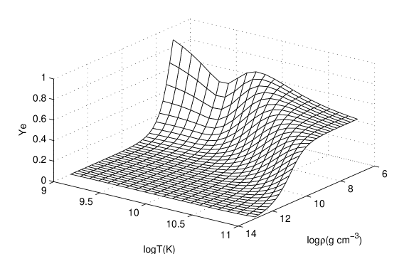
Figure 1: electron fraction $Y_{e}$ as a function of $T$ and $\rho$ for equilibrium state $npe^{\pm}$ gas.

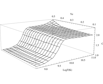
Figure 2: the coefficient $C$ of chemical potential equilibrium condition $\mu_{n}=\mu_{p}+C\mu_{e}$ as a function of $T$ and $Y_{e}$.

As an example, we introduce the application to electron fraction of GRB accretion disk. GRB is one of the most violent events in the universe, but its explosion mechanism is still not clear. Many authors support the view that GRB originates from the accretion disk of stellar mass black hole. Various accretion rates (from $0.01M_{\odot}\,s^{-1}$ to 10$M_{\odot}\,s^{-1}$) bring quite significant difference to the disk structure and composition. As the temperature of the accretion disk is generally larger than $10^{10}K$, all nuclei are dissociated to the free nucleons, so $npe^{\pm}$ gas can describe the composition well. For lower accretion rates ($\dot{M}\leq 0.1M_{\odot}\,s^{-1}$), the disk is transparent to neutrinos and antineutrinos, and neutrino and antineutrino absorption are not important(Surman & McLaughlin, 2004). Adopting the steady equilibrium condition, $Y_{e}$ of the disk model PWF99(Popham et al., 1999)(accretion rate $\dot{M}=0.1M_{\odot}\,s^{-1}$, alpha viscosity $\alpha=0.1$, and black hole spin parameter $a=0.95$) are obtained in Fig.3. Dashed line and solid line are the result from the steady equilibrium condition and the full calculation by Surman et al. respectively. It shows that in the inner region of disk(from 20km to 120km), electron fraction from different methods are conform principally, which indicates the composition in the disk is in approximate equilibrium state, but our result is generally smaller than that of Surman et al. While in outer region of the disk, $Y_{e}$ deviates from equilibrium, and this deviation increases with the accretion disk radius.

Surman and McLaughlin (2004) did not bother with specifying the radial profile of the temperature and the density of the accretion disk when calculating the electron fraction as a function of the radius for model introduced by Popham et al (1999). Here we rewrite the temperature and the density formulae of Popham et al. (1999)’s analytical model as

$$T=1.3\times 10^{11}\alpha^{0.2}M_{1}^{-0.2}R^{-0.3}\rm K$$ (14)

$$\rho=1.2\times 10^{14}\alpha^{-1.3}M_{1}^{-1.7}R^{-2.55}\dot{M}_{1}\rm g\,cm^{-3}$$ (15)

where $M_{1}$ is the mass of the accreting black hole in $M_{\odot}$, and $R$ is the radius in gravitational radius $r_{g}$ ($r_{g}\equiv GM_{1}/c^{2}$, which is equal to 1.4767km for $M_{1}=1M_{\odot}$). Since the explicit formulae are given, we adopt the equilibrium condition of $npe^{\pm}$ gas to obtain some representative values of $Y_{e}$ in Fig.4 at the radius larger than the inner edge (6 gravitational radius) of accretion disk. One can find from Fig.4 that $Y_{e}$ have a rapid increase with radius because both densities and temperatures decrease rapidly when radius increase and the variation of $Y_{e}$ is very sensitive to density and temperature as shown in Fig. 1. For the different accretion rate, the accretion rate is larger, the $Y_{e}$ is larger. This means the distribution of $Y_{e}$ along the radius highly depends on the structure equations of the disk.

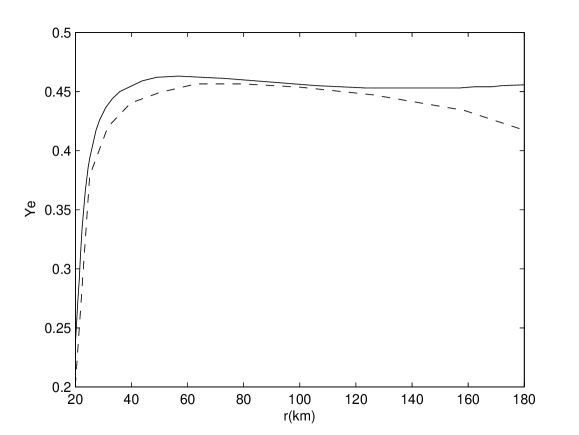
Figure 3: $Y_{e}$ as a function of accrection disk radius for model $\dot{M}=0.1$, alpha viscosity $\alpha=0.1$, and black hole spin parameter a=0.95. The dashed line shows $Y_{e}$ from steady equilibrium condition, while the solid line is the full calculation by Surman et al.(Surman & McLaughlin, 2004)

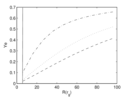
Figure 4: $Y_{e}$ as a function of accrection disk radius for the thin disk analytical model($\alpha$=0.1, a=0, $M_{1}$=3). Long-dashed line, dotted line and dot-dashed line show $Y_{e}$ as the accretion rate $\dot{M}$ =0.01, 0.05, 0.1, respectively. Vertical solid line denotes the inner boundary of the accretion disk (6 gravitational radius).

Table 3: steady state chemical equilibrium condition as neutrino opaque for $T=5\times 10^{10}\rm K$. The notes are the same as those in Table 1.

$Y_{e}$	$\rho$	$\lambda_{e^{-}p}$	$\lambda_{\nu_{e}n}$	$\lambda_{e^{+}n}$	$\lambda_{\bar{\nu}_{e}p}$	$\lambda_{n}$	$\mu_{e}^{{}^{\prime}}$	$\mu_{n}^{{}^{\prime}}$	$\mu_{p}^{{}^{\prime}}$	$C$
	$\rm g\,cm^{-3}$	$\rm cm^{-3}\,s^{-1}$	$\rm cm^{-3}\,s^{-1}$	$\rm cm^{-3}\,s^{-1}$	$\rm cm^{-3}\,s^{-1}$	$\rm cm^{-3}\,s^{-1}$	$\rm MeV$	$\rm MeV$	$\rm MeV$
0.10	2.32E+11	7.92E+37	7.89E+37	7.88E+36	7.56E+36	1.23E+31	10.18	-15.14	-24.65	1.01
0.20	6.17E+10	2.03E+37	2.01E+37	4.17E+36	4.01E+36	5.87E+30	6.69	-21.40	-27.38	1.01
0.30	2.46E+10	7.35E+36	7.26E+36	2.48E+36	2.39E+36	3.10E+30	4.37	-25.95	-29.60	1.01
0.40	1.05E+10	2.75E+36	2.71E+36	1.40E+36	1.35E+36	1.52E+30	2.48	-30.29	-32.03	1.01
0.50	3.40E+09	7.56E+35	7.40E+35	5.59E+35	5.43E+35	5.17E+29	0.75	-35.94	-35.93	1.02

2.2 Case 2. Neutrinos are Opaque

In the neutrino-opaque and antineutrino-opaque matter, neutrino and antineutrino will be absorbed by proton and neutron except the reactions (2)-(4) as following,

$$\nu_{e}+n\rightarrow e^{-}+p,$$ (16)

$$\bar{\nu}_{e}+p\rightarrow e^{+}+n.$$ (17)

By using sections $\sigma^{abs}_{\nu_{e}n}=\frac{A}{\pi^{2}}(E_{\nu_{e}}+Q)[(E_{\nu_{e}}+Q)^{2}-1]^{1/2}(1-f_{e})$ and $\sigma^{abs}_{\bar{\nu}_{e}p}=\frac{A}{\pi^{2}}(E_{\bar{\nu}_{e}}-Q)[(E_{\bar{\nu}_{e}}-Q)^{2}-1]^{1/2}(1-f_{e^{+}})$, we obtain their rates(the natural units system)

$$\lambda_{\nu_{e}n}=\frac{A}{2\pi^{4}}n_{n}\int_{0}^{\infty}(E_{\nu}+Q)[(E_{\nu_{e}}+Q)^{2}-1]^{1/2}F(Z+1,E_{\nu_{e}}+Q)(1-f_{e})E^{2}_{\nu_{e}}f_{\nu_{e}}dE_{\nu_{e}},$$ (18)

$$\lambda_{\bar{\nu}_{e}p}=\frac{A}{2\pi^{4}}n_{p}\int_{0}^{\infty}(E_{\bar{\nu}}-Q)[(E_{\bar{\nu}_{e}}-Q)^{2}-1]^{1/2}F(-Z+1,E_{\nu_{e}}-Q)(1-f_{e^{+}})E^{2}_{\bar{\nu}_{e}}f_{\bar{\nu}_{e}}d\bar{\nu}_{e},$$ (19)

where $f_{\nu_{e}}$ and $f_{\bar{\nu}_{e}}$ are the Fermi-Dirac distribution function of neutrino and antineutrino. $f_{\nu_{e}}=[1+\exp{(\frac{E_{\nu_{e}}-\mu_{\nu_{e}}}{kT})}]^{-1}$, $f_{\bar{\nu}_{e}}=[1+\exp{(\frac{E_{\bar{\nu}_{e}}-\mu_{\bar{\nu}_{e}}}{kT})}]^{-1}$. The number densities of neutrino and antineutrino are

$$n_{\nu_{e}}-n_{\bar{\nu}_{e}}=\frac{4\pi}{h^{3}}\int p^{2}dp\frac{1}{1+\exp{(\frac{E_{\nu_{e}}-\mu_{\nu_{e}}}{kT})}}-\frac{4\pi}{h^{3}}\int p^{2}dp\frac{1}{1+\exp{(\frac{E_{\bar{\nu}_{e}}+\mu_{\nu_{e}}}{kT})}}.$$ (20)

When $n_{\nu_{e}}=n_{\bar{\nu}_{e}}$, i.e. number density of neutrino is equal to that of antineutrino, $\mu_{\nu_{e}}=\mu_{\bar{\nu}_{e}}=0$. In this case, the equilibrium condition Eq.(5) becomes

$$\lambda_{e^{-}p}-\lambda_{\nu_{e}n}=\lambda_{e^{+}n}-\lambda_{\bar{\nu}_{e}p}+\lambda_{n}.$$ (21)

One can find from Table 3 that even at $T=5\times 10^{10}$K, $C$ is still approximate to 1. In another word, for a system with neutrino and antineutrino are opaque and their chemical potentials are zero, $\mu_{n}=\mu_{p}+\mu_{e}$ is always effective no matter what temperature is, just as expected.

Table 4: the evolution of initial electron fraction at different steady state chemical equilibrium conditions. $t$ is the time post bounce, $R_{\nu}$ is the neutrinospheric radius, $L_{n}$ is the number luminosity for neutrino and antineutrino, $<E_{\nu_{e}}>$ and $<E_{\bar{\nu}_{e}}>$ are the average energy of neutrino and antineutrino respectively. All parameters above refer to Ref.(Arcones et al., 2008)

$t$	$R_{\nu}$	$T$	$L_{n}$	$<E_{\nu_{e}}>$	$<E_{\bar{\nu}_{e}}>$	$\rho$	$Y_{e}^{a}$	$Y_{e}^{b}$	$C$
$s$	$\rm km$	$\rm MeV$	$\rm 10^{56}s^{-1}$	$\rm MeV$	$\rm MeV$	$\rm gcm^{-3}$
2	10.55	6.34	6.05	20.71	25.64	5.50E+11	0.113	0.084	1.39
5	9.82	5.14	3.55	17.1	22.6	1.30E+12	0.050	0.039	1.22
7	9.68	4.73	3.03	15.9	21.69	1.40E+12	0.042	0.035	1.15
10	9.59	4.37	3.06	15.05	21.86	2.00E+12	0.029	0.028	1.03

3 Equilibrium Condition of $npe^{\pm}$ Gas with External Neutrino Flux

As discussed in Section 2, we only consider that $npe^{\pm}$ gas is isolated, but for many astrophysical environments, the external strong neutrino and antineutrino fluxes can not be ignored. These processes involve some complex and difficult problems that concern both the neutrino transport and the interactions with nucleons. Here we discuss the neutrino-driven wind (NDW) from proto-neutron star (PNS) as a typical example. NDW is regarded as the major site for the r-process nucleosynthesis according to the observations of metal-poor-star in the recent years (see e.g., Qian, 2008, 2000; Martínez-Pinedo, 2008). Since the NDW is firstly proposed by Duncan et al. in 1986 (Duncan et al., 1986), many detailed analysis for this process have been done by many authors, including Newtonian and general relativity hydrodynamics and the other physical inputs, e.g. rotating, magnetic field, termination shock and so on(Qian & Woosley, 1996; Thompson, 2003; Metzger et al., 2007; Kuroda et al., 2008; Thompson et al., 2001; Fischer et al., 2009). A basic scenario of r-process nucleosynsis in the NDW can be simply described as(see Martínez-Pinedo, 2008): soon after the birth of PNS, lots of neutrinos are emitted from the surface of PNS; because of the photodisintegration of shock wave, the main composition at the surface of PNS is proton, neutron, electron and positron (i.e. $npe^{\pm}\rm\,gas$); in the circumambience of PNS, the main reactions are the neutrino or antineutrino’s absorption and emitting by nucleons (so called ’ neutrino heat region’); in the further region electron fraction $Y_{e}$ keeps as a constant and $\alpha$ particles are combined; above this region, other particles, such as ${}^{12}\rm C,\,^{9}\rm Be$, are produced till the seed nuclei; abundant neutrinos are captured by seed nuclei in succession. The previous researches show that the steady state is a good approximation to the NDW in the first 20 seconds(Thompson et al., 2001; Thompson, 2003; Qian & Woosley, 1996; Fischer et al., 2009);

Usually, neutron-to-seed ratio, electron fraction, entropy and expansion timescale are four essential parameters for a successful r-element pattern. It is very difficult to fulfill all those conditions self-consistently. Electron fraction $Y_{e}$ is one of the most important parameters. Recent research by Wanajo et al. shows that the puzzle of the excess of r-element of $A=90$ may be solved if $Y_{e}$ can increase 1-2%(Wanajo et al., 2009). The evolution of $Y_{e}$ is usually obtained by solving the differential equation group which is related to the EoS, neutrino reaction rates and hydrodynamic frame(Thompson et al., 2001). Initial $Y_{e}$ at the origin of wind is an important boundary condition. Considering the neutrinos are emitted from the neutrino sphere, $Y_{e}$ at neutrino sphere can be regarded as the initial $Y_{e}$ of the wind. For a given model, the initial $Y_{e}$ can be determined by making the assumption that the matter in neutrino sphere is in beta equilibrium(Arcones et al., 2008). To compare the results with the previous work of Arcones et al., we employs the same PNS model M15-l1-r1 (Arcones et al., 2008, 2007). The model has a baryonic mass of 1.4 $\rm M_{\odot}$, obtained in a spherically symmetric simulation of the parameterized 15 $\rm M_{\odot}$ supernova explosion model. Detailed research shows that there are a few $\alpha$ particles will appear at the neutrino sphere, but number density of $\alpha$ particle is much smaller than that of proton and neutron, so it is reasonable to ignore the $\alpha$ particle effect on electron fraction, i.e., the matter is regarded as $npe^{\pm}$ gas. Simultaneity, although lots of neutrino and antineutrino are emitted from PNS, their number densities are equal, which means $\mu_{\nu_{e}}=\mu_{\bar{\nu}_{e}}=0$. Since the neutrino and antineutrino are transparent to the matter at neutrino sphere, neutrino produced by reactions (2)-(3) can not interact with nucleons, but for the neutrino and antineutrino come from the core region of PNS, absorption reactions (16) and (17) are permitted. Their rates are

$$\lambda_{\nu_{e}n}=\frac{L_{n,\nu_{e}}}{4\pi R_{\nu}^{2}}\sigma_{\nu_{e}n}^{abs}\rho(1-Y_{e})N_{A},$$ (22)

$$\lambda_{\bar{\nu}_{e}p}=\frac{L_{n,\bar{\nu}_{e}}}{4\pi R_{\nu}^{2}}\sigma_{\bar{\nu}_{e}p}^{abs}\rho Y_{e}N_{A},$$ (23)

where $L_{n,\nu}$ and $L_{n,\bar{\nu}_{e}}$ are the number luminosity of neutrino and antineutrino respectively, $R_{\nu}$ is the neutrinospheric radius. Considering too many physical factors (EOS , transport equation and so on) will influence the number luminosity and the neutrino energy, we simply assume the number luminosity and the energy of neutrino and antineutrino are the same as those in the wind. Firstly, we obtain the electron fraction by using a general equilibrium condition $\lambda_{e^{-}p}-\lambda_{\nu_{e}n}=\lambda_{e^{+}n}-\lambda_{\bar{\nu}_{e}p}+\lambda_{n}$. In other words, if the density and temperature are fixed for the equilibrium system, the electron fraction is unique. Then the coefficient $C$ in the chemical potential equilibrium condition is determined (leftmost column in Table 4) . The results for model M15-l1-r1 are shown in Table 4. $Y_{e}^{a}$ is the electron fraction for an extreme case $C=1$, which is adopted in reference (Arcones et al., 2008); $Y_{e}^{b}$ is the result in which the steady equilibrium condition is valid and the external neutrino flux is also considered. We can find $Y_{e}^{b}$ is universal smaller than $Y_{e}^{a}$, which means the external neutrino flux strongly influences the composition of equilibrium system. Comparing $Y_{e}^{a}$ with $Y_{e}^{b}$, one can find that the improved equilibrium condition makes the electron fraction decrease significantly when the time is less than 5 seconds post bounce. After 5 seconds the electron fractions are similar to the case $C=1$. Note that it is just a conclusion for the model M15-l1-r1. Due to the huge difference between the different models, the results may be quite different for the other models. More detailed consideration will be done in our further work. Initial electron fraction is an important boundary condition to determine the electron fraction of the wind. Since r-process nucleosynthesis is strongly dependant on the electron fraction, the accurate electron fraction is useful for the final r-process nucleosynthesis.

4 Conclusions

In this work, we derive the chemical potential equilibrium conditions $\mu_{n}=\mu_{p}+C\mu_{e}$ for $npe^{\pm}$ gas at two cases ( with/without external neutrino flux). Especially in the neutrino-transparent matter, employing the fitting Eq.(13) for the transition from low temperature and high temperature is a more convenient method than the calculation of interaction rates as usual. Since chemical potentials are dependant on three parameters: density, electron fraction and temperature, any one of those three parameters can be determined if the other two parameters are given. Although the variation of factor $C$ is complicated as the external neutrino flux cannot be ignored, one can obtain the extremum of those parameters assuming the $C=1$ or 2. Furthermore, our results can be regarded as the reference value for non-equilibrium sates. Considering the simplicity and the far-ranging astrophysical environment, the results in this paper is expected to be used widely in the further relative works.

ACKNOWLEDGEMENTS

The author would like to thank Prof. Yuan Y.-F. for many valuable conversations and help with preparing this manuscript, and the referee for his/her constructive suggestions which are helpful to improve this manuscript.

References

- Arcones et al. (2007) Arcones, A., Janka, H.-T., & Scheck, L. 2007, A&A, 467, 1227
- Arcones et al. (2008) Arcones, A., Martínez-Pinedo, G., O’Connor, E., Schwenk, A., Janka, H.-T., Horowitz, C. J., & Langanke, K. 2008, Phys. Rev. C, 78, 015806
- Baldo & Ducoin (2009) Baldo, M., & Ducoin, C. 2009, Phys. Rev. C, 79, 035801
- Cheng et al. (2009) Cheng, K. S., Harko, T., Huang, Y. F., Lin, L. M., Suen, W. M., & Tian, X. L. 2009, Journal of Cosmology and Astro-Particle Physics, 9, 7
- Duncan et al. (1986) Duncan, R. C., Shapiro, S. L., & Wasserman, I. 1986, ApJ, 309, 141
- Dutta et al. (2004) Dutta, S. I., Ratković, S., & Prakash, M. 2004, Phys. Rev. D, 69, 023005
- Fischer et al. (2009) Fischer, T., Whitehouse, S. C., Mezzacappa, A., Thielemann, F. -., & Liebendörfer, M. 2009, arXiv:0908.1871
- Harwit (2006) Harwit, M. 2006, Astrophysical Concepts(4rd ed), (New York:Springer-Verlag), 544
- Janiuk & Yuan (2010) Janiuk, A., & Yuan, Y.-F. 2010, A&A, 509, A260000
- Janka (2001) Janka, H.-T. 2001, A&A, 368, 527
- Kippenhanhn & Weigert (1990) Kippenhahn, R., & Weigert, A. 1990, Stellar Structure and Evolution, (Berlin Heidelberg:Springer-Verlag),169
- Kuroda et al. (2008) Kuroda, T., Wanajo, S., & Nomoto, K. 2008, ApJ, 672, 1068
- Lai & Qian (1998) Lai, D., & Qian, Y.-Z. 1998, ApJ, 505, 844
- Langanke & Martínez-Pinedo (2000) Langanke, K., & Martínez-Pinedo, G. 2000, Nuclear Physics A, 673, 481
- Liu et al. (2007) Liu, T., Gu, W.-M., Xue, L., & Lu, J.-F. 2007, ApJ, 661, 1025
- Marek & Janka (2009) Marek, A., & Janka, H.-T. 2009, ApJ, 694, 664
- Martínez-Pinedo (2008) Martínez-Pinedo, G. 2008, European Physical Journal Special Topics, 156, 123
- Metzger et al. (2007) Metzger, B. D., Thompson, T. A., & Quataert, E. 2007, ApJ, 659, 561
- Popham et al. (1999) Popham, R., Woosley, S. E., & Fryer, C. 1999, ApJ, 518, 356
- Pruet & Dalal (2002) Pruet, J., & Dalal, N. 2002, ApJ, 573, 770
- Qian & Woosley (1996) Qian, Y.-Z., & Woosley, S. E. 1996, ApJ, 471, 331
- Qian (2000) Qian, Y.-Z. 2000, ApJ, 534, L67
- Qian (2008) Qian Y.-Z. 2008, arXiv:0809.2826
- Reddy et al. (1998) Reddy, S., Prakash, M., & Lattimer, J. M. 1998, Phys. Rev. D, 58, 013009
- Shapiro & Teukolsky (1983) Shapiro, S.L., & Teukolsky, S.A. 1983, Black Holes, White Dwarfs and Neutron Stars, (New York: John Wiley Sons), 39
- Surman & McLaughlin (2004) Surman, R., & McLaughlin, G. C. 2004, ApJ, 603, 611
- Thompson et al. (2001) Thompson, T. A., Burrows, A., & Meyer, B. S. 2001, ApJ, 562, 887
- Thompson (2003) Thompson, T. A. 2003, ApJ, 585, L33
- Wanajo et al. (2009) Wanajo, S., Nomoto, K., Janka, H.-T., Kitaura, F. S., Müller, B. 2009, ApJ, 695, 208
- Yakovlev et al. (2008) Yakovlev, D. G., Gnedin, O. Y., Kaminker, A. D., & Potekhin, A. Y. 2008, 40 Years of Pulsars: Millisecond Pulsars, Magnetars and More, 983, 379
- Yuan (2005) Yuan, Y.-F. 2005, Phys. Rev. D, 72, 013007