Current cosmological constraints on the curvature, dark energy and modified gravity

Abstract

We apply the Union2 compilation of 557 supernova Ia data, the baryon acoustic oscillation measurement of distance, the cosmic microwave background radiation data from the seven year Wilkinson Microwave Anisotropy Probe, and the Hubble parameter data to study the geometry of the Universe and the property of dark energy by using models and parametrizations with different high redshift behaviours of $w(z)$. We find that $\Lambda$CDM model is consistent with current data, that the Dvali-Gabadadze-Porrati model is excluded by the data at more than $3\sigma$ level, that the Universe is almost flat, and that the current data is unable to distinguish models with different behaviours of $w(z)$ at high redshift. We also add the growth factor data to constrain the growth index of Dvali-Gabadadze-Porrati model and find that it is more than $1\sigma$ away from its theoretical value.

1 Introduction

Even since the discovery of the accelerated expansion of the Universe in 1998 (Riess et al., 1998; Perlmutter et al., 1999), many efforts have been made to confirm and understand this phenomenon of acceleration. For the explanation of the acceleration, there are three different approaches. The first method introduces a new exotic form of matter with negative pressure, dubbed as dark energy to drive the Universe to accelerate. The cosmological constant is the simplest candidate of dark energy which is also consistent with observations, but at odds with quantum field theory. The second method modifies the theory of gravity known as general relativity at the cosmological scale, such as the Dvali-Gabadadze-Porrati (DGP) model (Dvali, Gabadadze & Porrati, 2000). The third approach takes the view that the Universe is inhomogeneous. In this paper, we focus on dark energy and DGP models.

The only effect of dark energy we know is through gravitational interaction; this makes it difficult to understand the physical nature of dark energy. In particular, the question whether dark energy is the cosmological constant remains unanswered. Recently, it was claimed that the flat $\Lambda$CDM model is inconsistent with observations at more than $1\sigma$ level (Huang et al., 2009; Shafieloo, Sahni & Starobinsky, 2009; Cai, Su & Zhang, 2010). Shafieloo, Sahni & Starobinsky (2009) suggested that the cosmic acceleration is slowing down from $z\sim 0.3$. In Huang et al. (2009), it was claimed that dark energy suddenly emerged at redshift $z\sim 0.3$. Cai, Su & Zhang (2010) found possible oscillating behaviour of dark energy. However, no evidence for dark energy dynamics was found in other studies (Lampeitl et al., 2009; Serra et al., 2009; Gong et al., 2010a; Gong, Wang & Cai, 2010b; Pan et al., 2010). The difference between the conclusions drawn in Shafieloo, Sahni & Starobinsky (2009) and Gong et al. (2010a) lies in the Baryon Acoustic Oscillation (BAO) data used in their analysis. Shafieloo, Sahni & Starobinsky (2009) employs the ratio $D_{V}(0.35)/D_{V}(0.2)$ of the effective distance $D_{V}(z)$ at two redshifts, while Gong et al. (2010a) applies the BAO $A$ parameter given by Eisenstein et al. (2005). The tension between BAO measurement and higher redshift type Ia supernova (SN Ia) was noticed in Percival et al. (2007), and the tension was lessened in Percival et al. (2010) due to revised error analysis, different methodology adopted and more data.

It was argued that the systematics in different data sets heavily affected the fitting results (Hicken et al., 2009; Sollerman et al., 2009; Gong, Wang & Cai, 2010b; Kessler et al., 2010). The Constitution compilation found that the scatter at high redshift is higher for SALT and SALT2 fitters, and SALT2 poorly fits the nearby U-band light curves (Hicken et al., 2009). However, it was found that SALT2 performs better than SALT and MLCS2k2 judged by the scatter around the best-fitting luminosity distance relationship in Conley et al. (2008) and Amanullah et al. (2010). Because MLCS2k2 training is mainly based on the observation of nearby SN Ia, and because the observations made in the observer-frame U-band are contaminated with a high level of uncertainty due to atmospheric variations, so MLCS2k2 is less accurate at predicting the rest-frame U-band using high redshift SN Ia (Amanullah et al., 2010; Kessler et al., 2010). The Union2 data applies the SALT2 light curve fitter because it addresses the problem by including high redshift data where the rest-frame U-band is observed at redder wavelengths (Amanullah et al., 2010). In this paper, we combine the Union2 sample of 557 SN Ia data with systematic errors (Amanullah et al., 2010), the BAO distance ratios $r_{s}(z_{d})/D_{V}(z)$ between the comoving sound horizon at the baryon drag epoch $r_{s}(z_{d})$ and the effective distance $D_{V}(z)$ at $z=0.2$ and $z=0.35$ (Percival et al., 2010), the radial BAO measurements at $z=0.24$ and $z=0.43$ (Gaztañaga, Miquel & Sánchez, 2009a), the seven-year Wilkinson Microwave Anisotropy Probe (WMAP7) data (Komatsu et al., 2011), and the Hubble parameter $H(z)$ data (Gaztañaga, Cabré & Hui, 2009b; Stern et al., 2010) to probe the geometry of the Universe and the nature of dark energy with different models.

The paper is organised as follows. In section 2, we present the SN Ia data (Amanullah et al., 2010), the BAO data (Gaztañaga, Miquel & Sánchez, 2009a; Percival et al., 2010), the WMAP7 data (Komatsu et al., 2011), the $H(z)$ data (Gaztañaga, Cabré & Hui, 2009b; Stern et al., 2010), and the growth factor data (Viel, Haehnelt & Springel, 2004, 2006; McDonald et al., 2005; Tegmark el al., 2006; Ross et al., 2007; Ângela et al., 2008; Guzzo et al., 2008; Blake et al., 2010), and all the formulae related to these data. In section 3, we list all the models and the fitting results, and conclusions are given in section 4.

2 Observational data

The Union2 SN Ia data consist of the low-$z$ SN Ia data observed at the F.L. Whipple observatory of the Harvard-Smithsonian centre for astrophysics (Hicken et al., 2009), the intermediate-$z$ data observed during the first season of the Sloan Digital Sky Survey (SDSS)-II supernova survey (Kessler et al., 2010), and the high-$z$ data from the Union compilation (Kowalski et al., 2008). The Union2 SN Ia data used the SALT2 light-curve fitter because it performs better than both SALT and MLCS2k2 when judged by the scatter around the best-fitting luminosity distance relationship (Amanullah et al., 2010). To use the 557 Union2 SN Ia data (Amanullah et al., 2010), we minimize

$$\chi^{2}=\sum_{i,j=1}^{557}[\mu(z_{i})-\mu_{obs}(z_{i})]C^{-1}_{sn}(z_{i},z_{j})[\mu(z_{j})-\mu_{obs}(z_{j})],$$ (1)

where the extinction-corrected distance modulus $\mu(z)=5\log_{10}[d_{L}(z)/{\rm Mpc}]+25$, $C_{sn}(z_{i},z_{j})$ is the covariant matrix which includes the systematical errors for the SN Ia data (Amanullah et al., 2010); the covariant matrix is available online. The luminosity distance $d_{L}(z)$ is

$$d_{L}(z)=\frac{1+z}{H_{0}\sqrt{|\Omega_{k}|}}\,S_{k}\!\left[\sqrt{|\Omega_{k}|}\int_{0}^{z}\frac{dx}{E(x)}\right],$$ (2)

the dimensionless Hubble parameter $E(z)=H(z)/H_{0}$; and $S_{k}(x)$ is defined as $x$, $\sin(x)$ or $\sinh(x)$ for $k=0$, +1, or -1, respectively. Due to the arbitrary normalization of the luminosity distance, the nuisance parameter $h=H_{0}/$(100 km s^-1Mpc^-1) in the SN Ia data is not the observed Hubble constant. So we marginalize the nuisance parameter $h$ with a flat prior, after the marginalization, we get (Gong, Wu & Wang, 2008)

$$\begin{array}[]{ll}\chi^{2}_{sn}(\mathbf{p})=&\sum_{ij}\alpha_{i}C^{-1}_{sn}(z_{i},z_{j})\alpha_{j}\\ &-\frac{\left[\sum_{ij}\alpha_{i}C^{-1}_{sn}(z_{i},z_{j})-\ln 10/5\right]^{2}}{\sum_{ij}C^{-1}_{sn}(z_{i},z_{j})}\\ &-2\ln\left(\frac{\ln 10}{5}\sqrt{\frac{2{\rm\pi}}{\sum_{ij}C^{-1}_{sn}(z_{i},z_{j})}}\right),\end{array}$$ (6)

where $\alpha_{i}=\mu_{obs}(z_{i})-25-5\log_{10}[H_{0}d_{L}(z_{i})]$.

In addition to the Union2 SN Ia data, we use the BAO distance measurement from the oscillations in the distribution of galaxies. The BAO is due to the sound waves in the plasma of the early Universe and the wavelength of the BAO is related to the comoving sound horizon at the baryon drag epoch. The distance at the redshift $z=0.2$ was measured in the clustering of the combined 2dF Galaxy Redshift Survey (2dFGRS) and SDSS main galaxy samples, and the distance at the redshift $z=0.35$ was measured in the clustering of the SDSS luminous red galaxies. From the BAO observation of the galaxy power spectra, Percival et al. (2010) measured the distance ratio,

$$d_{z}=\frac{r_{s}(z_{d})}{D_{V}(z)}$$ (7)

at two redshifts $z=0.2$ and $z=0.35$ to be $d_{0.2}^{obs}=0.1905\pm 0.0061$, and $d_{0.35}^{obs}=0.1097\pm 0.0036$ (hereafter Bao2). Here the effective distance is

$$D_{V}(z)=\left[\frac{d_{L}^{2}(z)}{(1+z)^{2}}\frac{z}{H(z)}\right]^{1/3},$$ (8)

$z_{d}$ is the drag redshift defined in Eisenstein & Hu (1998), the comoving sound horizon is

$$r_{s}(z)=\int_{z}^{\infty}\frac{c_{s}(x)dx}{E(x)},$$ (9)

where the sound speed $c_{s}(z)=1/\sqrt{3[1+\bar{R_{b}}/(1+z)}]$, and $\bar{R_{b}}=3\Omega_{b}h^{2}/(4\times 2.469\times 10^{-5})$. To use this BAO data, we calculate

$$\chi^{2}_{Bao2}(\mathbf{p},\Omega_{b}h^{2},h)=\sum_{i,j=1}^{2}\Delta d_{i}C_{Bao}^{-1}(d_{i},d_{j})\Delta d_{j},$$ (10)

where $d_{i}=(d_{z=0.2},d_{z=0.35})$, $\Delta d_{i}=d_{i}-d_{i}^{obs}$ and the covariance matrix $C_{Bao}(d_{i},d_{j})$ for the two parameters $d_{0.2}$ and $d_{0.35}$ is taken from equation (5) in Percival et al. (2010). Besides the model parameters $\mathbf{p}$, we need to add two more nuisance parameters $\Omega_{b}h^{2}$ and $\Omega_{m}h^{2}$ when we use the BAO data.

From the measurement of the radial (line-of-sight) BAO scale in the galaxy power spectra, the cosmological parameters may be determined from the measured values of

$$\Delta z_{Bao}(z)=\frac{H(z)r_{s}(z_{d})}{c}$$ (11)

at two redshifts $z=0.24$ and $z=0.43$, which are $\Delta z_{Bao}(z=0.24)=0.0407\pm 0.0011$ and $\Delta z_{Bao}(z=0.43)=0.0442\pm 0.0015$ (hereafter Baoz), respectively (Gaztañaga, Miquel & Sánchez, 2009a). Therefore, we add $\chi^{2}$ with

$$\begin{array}[]{ll}\chi^{2}_{Baoz}(\mathbf{p},\Omega_{b}h^{2},h)=&\left(\frac{\Delta z_{Bao}(0.24)-0.0407}{0.0011}\right)^{2}\\ &+\left(\frac{\Delta z_{Bao}(0.43)-0.0442}{0.0015}\right)^{2}.\end{array}$$ (14)

When we add this BAO data to the fitting, we also need to add the nuisance parameters $\Omega_{b}h^{2}$ and $\Omega_{m}h^{2}$. In Gong, Wang & Cai (2010b), it was found that the Baoz data is consistent with the Bao2 data, and the constraints on the model parameters get improved with the addition of the Baoz data.

Because both the SN Ia and the BAO data measure the distance up to redshit $z<2$, we need to add distance data at higher redshift $z>10$ to better constrain the property of dark energy, so we use the WMAP7 data. When the full WMAP7 data are applied, we need to add some more parameters which depend on inflationary models, and this will limit our ability to constrain dark energy models. So we only use the WMAP7 measurements of the derived quantities such as the shift parameter $R(z^{*})$ and the acoustic scale $l_{A}(z^{*})$ at the decoupling redshift, and the decoupling redshift $z^{*}$. Then we add the following term to $\chi^{2}$,

$$\chi^{2}_{CMB}(\mathbf{p},\Omega_{b}h^{2},h)=\sum_{i,j=1}^{3}\Delta x_{i}C_{CMB}^{-1}(x_{i},x_{j})\Delta x_{j},$$ (15)

where the three parameters $x_{i}=[R(z^{*}),\ l_{A}(z^{*}),\ z^{*}]$, $\Delta x_{i}=x_{i}-x_{i}^{obs}$ and the covariance matrix $C_{CMB}(x_{i},x_{j})$ for the three parameters is taken from Table 10 in Komatsu et al. (2011). The shift parameter $R$ is expressed as

$$R(z^{*})=\frac{\sqrt{\Omega_{m}}}{\sqrt{|\Omega_{k}|}}S_{k}\!\left(\sqrt{|\Omega_{k}|}\int_{0}^{z^{*}}\frac{dz}{E(z)}\right)=1.725\pm 0.018.$$ (16)

The acoustic scale $l_{A}$ is

$$l_{A}(z^{*})=\frac{{\rm\pi}d_{L}(z^{*})}{(1+z^{*})r_{s}(z^{*})}=302.09\pm 0.76,$$ (17)

and $z^{*}$ is the decoupling redshift with the parametrization defined in Hu & Sugiyama (1996). We also need to add the parameters $\Omega_{b}h^{2}$ and $\Omega_{m}h^{2}$ to the parameter space when we employ the WMAP7 data.

The SN Ia, BAO and WMAP7 data measured the distance which depends on the double integration of the equation of state parameter $w(z)$, the process of double integration smoothes out the variation of equation of state parameter $w(z)$ of dark energy. To alleviate the double integration, we also apply the measurements of the Hubble parameter $H(z)$ which depends on $\Omega_{DE}$ directly and detects the variation of $w(z)$ better than the distance scales. Furthermore, the addition of the $H(z)$ data can better constrain $w(z)$ at high redshift (Gong et al., 2010a). In this paper, we use the $H(z)$ data at 11 different redshifts obtained from the differential ages of red-envelope galaxies in Stern et al. (2010), and three more Hubble parameter data $H(z=0.24)=76.69\pm 2.32$, $H(z=0.34)=83.8\pm 2.96$ and $H(z=0.43)=86.45\pm 3.27$, determined by Gaztañaga, Cabré & Hui (2009b). So we add these $H(z)$ data to $\chi^{2}$,

$$\chi^{2}_{H}(\mathbf{p},h)=\sum_{i=1}^{14}\frac{[H(z_{i})-H_{obs}(z_{i})]^{2}}{\sigma_{hi}^{2}},$$ (18)

where $\sigma_{hi}$ is the $1\sigma$ uncertainty in the $H(z)$ data. Basically, The model parameters $\mathbf{p}$ are determined by minimizing

$$\chi^{2}=\chi^{2}_{sn}+\chi^{2}_{Bao2}+\chi^{2}_{Baoz}+\chi^{2}_{CMB}+\chi^{2}_{H}.$$ (19)

In addition, we add the prior $h=0.742\pm 0.036$ (Riess et al., 2009).

In order to distinguish the modified gravity such as DGP model from dark energy models, we approximate the growth factor with $f(z)=\Omega_{m}^{\gamma}+(\gamma-4/7)\Omega_{k}$ (Gong, Ishak & Wang, 2009), then we use the growth factor data $f(z)$ obtained from the measurement of the redshift distortion to constrain the growth index $\gamma$ of the models (Viel, Haehnelt & Springel, 2004, 2006; McDonald et al., 2005; Tegmark el al., 2006; Ross et al., 2007; Ângela et al., 2008; Gong, 2008; Guzzo et al., 2008; Blake et al., 2010; Dossett et al., 2010). So we calculate

$$\chi^{2}_{f}(\mathbf{p},\gamma)=\sum_{i=1}^{15}\frac{[f(z_{i})-\Omega_{m}^{\gamma}(z_{i})-(\gamma-4/7)\Omega_{k}(z_{i})]^{2}}{\sigma_{f_{i}}^{2}}.$$ (20)

The likelihood for the parameters $\mathbf{p}$ in the model and the nuisance parameters is computed using the Monte Carlo Markov Chain (MCMC) method. The MCMC method randomly chooses values for the above parameters $\mathbf{p}$, evaluates $\chi^{2}$ and determines whether to accept or reject the set of parameters $\mathbf{p}$ using the Metropolis-Hastings algorithm. The set of parameters that are accepted to the chain forms a new starting point for the next process, and the process is repeated for a sufficient number of steps until the required convergence is reached. Our MCMC code is based on the publicly available package cosmomc (Lewis & Bridle, 2002; Gong, Wu & Wang, 2008).

After fitting the observational data to different dark energy models, we apply the $Om$ diagnostic (Sahni, Shafieloo & Starobinsky, 2008) to detect the deviation from the $\Lambda$CDM model. For a flat universe (Sahni, Shafieloo & Starobinsky, 2008),

$$Om(z)=\frac{E^{2}(z)-1}{(1+z)^{3}-1}.$$ (21)

For the $\Lambda$CDM model, $Om(z)=\Omega_{m}$ is a constant which is independent of the value of $\Omega_{m}$. Because of this property, $Om$ diagnostic is less sensitive to observational errors than the equation of state parameter $w(z)$ does. On the other hand, the bigger the value of $Om(z)$, the bigger the value of $w(z)$.

3 Cosmological models

3.1 $q_{1}-q_{2}$ parametrization

To understand the current accelerating expansion, we parametrize the deceleration parameter $q(z)$ with a simple two-parameter function (Gong & Wang, 2007),

$$q(z)=\frac{1}{2}+\frac{q_{1}z+q_{2}}{(1+z)^{2}}.$$ (22)

In this parametrization, we have only two parameters $\mathbf{p}=(q_{1},\ q_{2})$. The parameter $q_{2}=q(z=0)-1/2$, and $q(z)=1/2$ at high redshift which represents the matter dominated epoch. In principle, this parametrization does not involve $\Omega_{m}$ and $\Omega_{k}$, but the comoving distance depends on the geometry of the Universe through the function $S_{k}$, for simplicity, we consider the flat case $\Omega_{k}=0$ for this model. Although the flat assumption of $\Omega_{k}=0$ may induce large error in the estimation of cosmological parameters due to the degeneracy among $\Omega_{m}$, $\Omega_{k}$ and $w$ (Clarkson, Cortês & Bassett, 2007), but for this model, the only effect of $\Omega_{k}$ is through $S_{k}$, and $S_{k}(x)\approx x$ when $\Omega_{k}$ is small, so the impact of the flat assumption is small. The dimensionless Hubble parameter is

$$\begin{array}[]{ll}E(z)&=\exp\left[\int_{0}^{z}[1+q(u)]d\ln(1+u)\right]\\ &=(1+z)^{3/2}\exp\left[\frac{q_{2}}{2}+\frac{q_{1}z^{2}-q_{2}}{2(1+z)^{2}}\right].\end{array}$$ (25)

When $z\gg 1$, $E^{2}(z)\approx(1+z)^{3}\exp(q_{1}+q_{2})$, so we can think $q_{1}+q_{2}=\ln\Omega_{m}$. To account for the radiation-dominated Universe, we take the above $E(z)$ as the approximation for the matter and dark energy only, so we use the following Hubble parameter to approximate the whole expansion history of the Universe,

$$E^{2}(z)=\Omega_{r}(1+z)^{4}+(1+z)^{3}\exp\left[q_{2}+\frac{q_{1}z^{2}-q_{2}}{(1+z)^{2}}\right],$$ (26)

where the current radiation component $\Omega_{r}=4.1736\times 10^{-5}h^{-2}$ (Komatsu et al., 2011). Fitting the model to the combined SN Ia, Bao2, Baoz, WMAP7 and $H(z)$ data, we get the marginalized $1\sigma$ constraints, $q_{1}=0.07\pm 0.11$ and $q_{2}=-1.43\pm 0.09$ with $\chi^{2}=542.6$. In terms of $q_{0}=q(z=0)$, we find that $q_{0}<-0.62$ at $3\sigma$ confidence level, so the evidence of current acceleration is very strong. Furthermore, we find that the $3\sigma$ constraint on $\Omega_{m}$ is $\Omega_{m}=0.257_{-0.035}^{+0.044}$. The contour plot for $\Omega_{m}$ and $q_{0}$ is shown in Fig. 1(d).

At a low redshift, the radiation is negligible, so $Om(z)$ in this model is

$$Om(z)=\frac{(1+z)^{3}\exp[q_{2}+(q_{1}z^{2}-q_{2})/(1+z)^{2}]-1}{(1+z)^{3}-1}.$$ (27)

By using the best-fitting values of $q_{1}$ and $q_{2}$, we reconstruct $Om(z)$ and the results are plotted in Fig. 2(d).

3.2 Piecewise parametrization of $q(z)$

To further study the evolution of the deceleration parameter $q(z)$, we use the more model-independent piecewise parametrizations. We group the data into four bins so that the number of SN Ia in each bin times the width of each bin is around 30, i.e., $N\Delta z\sim 30$ and $N=4$. The four bins are $z_{1}=0.1$, $z_{2}=0.4$, $z_{3}=0.7$, $z_{4}=1.8$ and $z_{5}$ extends beyond 1089. For the redshift in the range $z_{i-1}\leq z<z_{i}$, the deceleration parameter $q(z)$ is a constant $q_{i}$, $q(z)=q_{i}$. Take $z_{0}=0$, then for $z_{i-1}\leq z<z_{i}$, we get

$$E(z)=(1+z)^{1+q_{N}}\prod_{i=1}^{N}(1+z_{i-1})^{q_{i-1}-q_{i}}.$$ (28)

In this model, we have four parameters $\mathbf{p}=(q_{1},\ q_{2},\ q_{3},\ q_{4})$. In general, for the piecewise parametrisation, the parameters such as $q_{i}$ in different bins are correlated and their errors depend upon each other. We follow Huterer & Cooray (2005) to transform the covariance matrix of $q_{i}$s to decorrelate the error estimate. Explicitly, the transformation is

$${\mathcal{Q}}_{i}=\sum_{j}T_{ij}q_{j},$$ (29)

where the transformation matrix $T=V^{T}\Gamma^{-1/2}V$, the orthogonal matrix $V$ diagonalizes the covariance matrix $C$ of $q_{i}$ and $\Gamma$ is the diagonalized matrix of $C$. For a given $i$, $T_{ij}$ can be thought of as weights for each $q_{j}$ in the transformation from $q_{i}$ to ${\mathcal{Q}}_{i}$. We are free to rescale each ${\mathcal{Q}}_{i}$ without changing the diagonality of the correlation matrix, so we then multiply both sides of the equation above by an amount such that the sum of the weights $\sum_{j}T_{ij}$ is equal to 1. This allows for easy interpretation of the weights as a kind of discretized window function. Now the transformation matrix element is $T_{ij}/\sum_{k}T_{ik}$ and the covariance matrix of the uncorrelated parameters is not the identity matrix. The $i$-th diagonal matrix element becomes $(\sum_{j}T_{ij})^{-2}$. In other words, the error of the uncorrelated parameters ${\mathcal{Q}}_{i}$ is $\sigma_{i}=1/\sum_{j}T_{ij}$. Fitting the model to the combined SN Ia, Bao2, Baoz, WMAP7 and $H(z)$ data, we get the constraints on the uncorrelated parameters $\mathcal{Q}_{i}$ and the result is shown in Fig. 3.

3.3 $\Lambda$CDM model

For the cosmological constant, the equation of state parameter $w=p/\rho=-1$, and the energy density $\rho_{\Lambda}$ is a constant. For a curved $\Lambda$CDM model, the curvature term $\Omega_{k}\neq 0$, Friedmann equation is

$$E^{2}(z)=\Omega_{k}(1+z)^{2}+\Omega_{m}(1+z)^{3}+\Omega_{r}(1+z)^{4}+\Omega_{\Lambda}.$$ (30)

At low redshits, the contribution of the radiation term is negligible. We have two parameters $\mathbf{p}=(\Omega_{m},\ \Omega_{k})$ and one nuisance parameter $h$ in this model. By fitting the $\Lambda$CDM model to the combined SN Ia, Bao2, Baoz, WMAP7 and $H(z)$ data, we get the marginalized $1\sigma$ constraints, $\Omega_{m}=0.272^{+0.013}_{-0.011}$ and $\Omega_{k}=0.002\pm 0.004$ with $\chi^{2}=541.2$. The contours of $\Omega_{m}$ and $\Omega_{k}$ are plotted in Fig. 4(a). By fitting the model to observational data combined with the growth factor data, the marginalized $1\sigma$ constraints are, $\Omega_{m}=0.272^{+0.013}_{-0.01}$, $\Omega_{k}=0.002\pm 0.004$ and $\gamma=0.56^{+0.14}_{-0.09}$ with $\chi^{2}=546.3$.

3.4 DGP model

In this model, gravity appears four dimensional at short distances while modified at large distances (Dvali, Gabadadze & Porrati, 2000). The model is motivated by brane cosmology in which our Universe is a three-brane embedded in a five dimensional spacetime. The Friedmann equation is modified as

$$E^{2}(z)=\Omega_{k}(1+z)^{2}+[\Omega_{d}+\sqrt{\Omega_{m}(1+z)^{3}+\Omega_{d}^{2}}\,]^{2},$$ (31)

where $\Omega_{d}=(1-\Omega_{m}-\Omega_{k})/2\sqrt{1-\Omega_{k}}$. If we take the point of view that Friedmann equation is not modified and the extra term in equation (31) is dark energy, then the equivalent dark energy equation of state parameter $w(z)$ for the DGP model is

$$w(z)=-\frac{\Omega_{m}(1+z)^{3}+2\Omega_{d}[\sqrt{\Omega_{m}(1+z)^{3}+\Omega_{d}^{2}}+\Omega_{d}]}{2[\Omega_{m}(1+z)^{3}+\Omega_{d}^{2}+\Omega_{d}\sqrt{\Omega_{m}(1+z)^{3}+\Omega_{d}^{2}}]}.$$ (32)

when $z\gg 1$, $w(z)\sim-1/2$ and $w(z=0)=-(1-\Omega_{k})/(1+\Omega_{m}-\Omega_{k})$. Since $\Omega_{k}$ is very small, $w(z)>-1$ for the DGP model.

By fitting the DGP model to the combined SN Ia, Bao2, Baoz, WMAP7 and $H(z)$ data, the marginalized $1\sigma$ constraints are $\Omega_{m}=0.288^{+0.015}_{-0.011}$ and $\Omega_{k}=0.019\pm 0.005$ with $\chi^{2}=561.6$. By fitting the DGP model to the combined SN Ia, Bao2, Baoz, WMAP7, $H(z)$, and $f(z)$ data, we get the marginalized $1\sigma$ estimations $\Omega_{m}=0.290^{+0.014}_{-0.012}$, $\Omega_{k}=0.019\pm 0.005$, and $\gamma=0.46^{+0.12}_{-0.08}$ with $\chi^{2}=567.5$.

3.5 CPL parametrization

For the Chevallier-Polarski-Linder (CPL) parametrization (Chevallier & Polarski, 2001; Linder, 2003), the equation of state parameter is

$$w(z)=w_{0}+\frac{w_{a}z}{1+z},$$ (33)

so $w(z=0)=w_{0}$ and $w(z)\sim w_{0}+w_{a}$ when $z\gg 1$. The corresponding dimensionless dark energy density is

$$\Omega_{DE}(z)=\Omega_{x}(1+z)^{3(1+w_{0}+w_{a})}{\rm e}^{[-3w_{a}z/(1+z)]},$$ (34)

where $\Omega_{x}=1-\Omega_{m}-\Omega_{r}-\Omega_{k}$. In this model, we have four model parameters $\mathbf{p}=(\Omega_{m},\ \Omega_{k},\ w_{0},\ w_{a})$. Fitting the model to the combined SN Ia, Bao2, Baoz, WMAP7 and $H(z)$ data, we get the marginalized $1\sigma$ constraints, $\Omega_{m}=0.265^{+0.019}_{-0.009}$, $\Omega_{k}=0.008^{+0.005}_{-0.011}$, $w_{0}=-1.16^{+0.26}_{-0.06}$, and $w_{a}=0.69^{+0.24}_{-1.41}$ with $\chi^{2}=540.5$. The contours of $w_{0}$ and $w_{a}$ are plotted in Fig. 1(a), and the contours of $\Omega_{m}$ and $\Omega_{k}$ are plotted in Fig. 4(b).

For the flat CPL model, $Om(z)$ becomes

$$Om(z)=\frac{\Omega_{m}(1+z)^{3}+\Omega_{DE}(z)-1}{(1+z)^{3}-1},$$ (35)

where $\Omega_{DE}(z)$ is defined in equation (34) with $\Omega_{k}=0$. By fitting the combined data to the flat CPL model, we get the marginalized $1\sigma$ constraints, $\Omega_{m}=0.267^{+0.019}_{-0.01}$, $w_{0}=-1.05^{+0.17}_{-0.1}$, and $w_{a}=0.07^{+0.32}_{-0.88}$ with $\chi^{2}=541.1$. Using this result, we reconstruct $Om(z)$ with equation (35) and the result is shown in Fig. 2(a).

3.6 JBP parametrization

For the Jassal-Bagla-Padmanabhan (JBP) parametrization (Jassal, Bagla & Padmanabhan, 2005), the equation of state parameter is

$$w(z)=w_{0}+\frac{w_{a}z}{(1+z)^{2}},$$ (36)

so $w(z=0)=w_{0}$ and $w(z)\sim w_{0}$ when $z\gg 1$. In this model, the parameter $w_{0}$ determines the property of the equation of state parameter $w(z)$ at both low and high redshifts. The corresponding dimensionless dark energy density is then

$$\Omega_{DE}(z)=\Omega_{x}(1+z)^{3(1+w_{0})}{\rm e}^{[3w_{a}z^{2}/2(1+z)^{2}]},$$ (37)

where $\Omega_{x}=1-\Omega_{m}-\Omega_{r}-\Omega_{k}$. In this model, we also have four parameters $\mathbf{p}=(\Omega_{m},\ \Omega_{k},\ w_{0},\ w_{a})$. Fitting the model to the combined SN Ia, Bao2, Baoz, WMAP7 and $H(z)$ data, we get the marginalized $1\sigma$ constraints, $\Omega_{m}=0.263^{+0.02}_{-0.01}$, $\Omega_{k}=0.004\pm 0.006$, $w_{0}=-1.21^{+0.32}_{-0.18}$, and $w_{a}=1.29^{+1.35}_{-2.33}$ with $\chi^{2}=540.6$. The contours of $\Omega_{m}$ and $\Omega_{k}$ are plotted in Fig. 4(c), and the contours of $w_{0}$ and $w_{a}$ are plotted in Fig. 1(b).

For the flat JBP model, $Om(z)$ becomes

$$Om(z)=\frac{\Omega_{m}(1+z)^{3}+\Omega_{DE}(z)-1}{(1+z)^{3}-1},$$ (38)

where $\Omega_{DE}(z)$ is defined in equation (37) with $\Omega_{k}=0$. By fitting the combined data to the flat JBP model, we get the marginalized $1\sigma$ constraints, $\Omega_{m}=0.265^{+0.019}_{-0.011}$, $w_{0}=-1.08^{+0.24}_{-0.19}$, and $w_{a}=0.32^{+1.01}_{-1.72}$ with $\chi^{2}=541.0$. Using this result, we reconstruct $Om(z)$ with equation (38) and the result is shown in Fig. 2(b).

3.7 Wetterich parametrization

Now we consider the parametrization proposed by Wetterich (2004),

$$w(z)=\frac{w_{0}}{[1+w_{a}\ln(1+z)]^{2}}.$$ (39)

For this model, $w(z=0)=w_{0}$ and $w(z)\sim 0$ when $z\gg 1$, so the behaviour of $w(z)$ at high redshift is limited. The dark energy density is

$$\Omega_{DE}=(1-\Omega_{m}-\Omega_{k}-\Omega_{r})(1+z)^{3+3w_{0}/[1+w_{a}\ln(1+z)]}.$$ (40)

In this model, the model parameters are $\mathbf{p}=(\Omega_{m},\ \Omega_{k},\ w_{0},\ w_{a})$. Fitting the model to the combined SN Ia, Bao2, Baoz, WMAP7 and $H(z)$ data, we get the marginalized $1\sigma$ constraints, $\Omega_{m}=0.264\pm 0.013$, $\Omega_{k}=0.009^{+0.014}_{-0.005}$, $w_{0}=-1.17^{+0.09}_{-0.23}$, and $w_{a}=0.32^{+0.46}_{-0.16}$ with $\chi^{2}=540.4$. The contours of $w_{0}$ and $w_{a}$ are plotted in Fig. 1(c), and the contours of $\Omega_{m}$ and $\Omega_{k}$ are plotted in Fig. 4(d).

For the flat Wetterich model, $Om(z)$ becomes

$$Om(z)=\frac{\Omega_{m}(1+z)^{3}+\Omega_{DE}(z)-1}{(1+z)^{3}-1},$$ (41)

where $\Omega_{DE}(z)$ is defined in equation (40) with $\Omega_{k}=0$. By fitting the combined data to the flat Wetterich model, we get the marginalized $1\sigma$ constraints, $\Omega_{m}=0.266^{+0.01}_{-0.015}$, $w_{0}=-1.05^{+0.02}_{-0.16}$, and $w_{a}=0.14\pm 0.1$ with $\chi^{2}=541.1$. Using this result, we reconstruct $Om(z)$ with equation (41) and the result is shown in Fig. 2(c).

3.8 Piecewise parametrization of $w(z)$

Finally, we consider a more model-independent parametrization of $w(z)$, the piecewise parametrization of $w(z)$. In this parametrization, the equation of state parameter is a constant, $w(z)=w_{i}$ for the redshift in the range $z_{i-1}<z<z_{i}$. For convenience, we choose $z_{0}=0$. We also assume that $w(z>1.8)=-1$. For a flat Universe, if $z_{i-1}\leq z<z_{i}$,

$$\Omega_{DE}(z)=(1-\Omega_{m})(1+z)^{3(1+w_{N})}\prod_{i=1}^{N}(1+z_{i-1})^{3(w_{i-1}-w_{i})}.$$ (42)

Again, the four parameters $w_{i}$ are correlated and we follow Huterer & Cooray (2005) to transform these parameters to decorrelated parameters $\mathcal{W}_{i}$. By fitting the model to the combined SN Ia, Bao2, Baoz, WMAP7 and $H(z)$ data, we get the error estimations of $\mathcal{W}_{i}$ and the results are shown in Fig. 5.

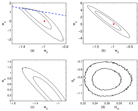
Figure 1: The marginalized $1\sigma$ and $2\sigma$ contour plots of $w_{0}$ ($\Omega_{m}$) and $w_{a}$ ($q_{0}$) for the CPL (a), JBP (b), Wetterich (c) and $q(z)$ (d) parametrisations. The dashed line in the upper left panel denotes the condition $w_{0}+w_{a}=0$.

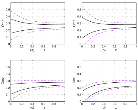
Figure 2: The marginalized $1\sigma$ and $2\sigma$ errors of $Om(z)$ for the CPL (a), JBP (b), Wetterich (c) and $q(z)$ (d) parametrisations.

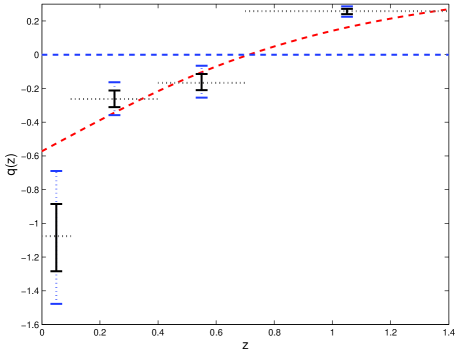
Figure 3: The $1\sigma$ and $2\sigma$ errors of the four uncorrelated $\mathcal{Q}_{i}$. The red dashed line is reconstructed with the best-fitting $\Lambda$CDM model.

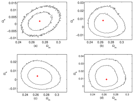
Figure 4: The marginalized $1\sigma$ and $2\sigma$ contour plots of $\Omega_{m}$ and $\Omega_{k}$ for the $\Lambda$CDM (a), CPL (b), JBP (c) and Wetterich (d) parametrisations. The red cross denotes the best-fitting value.

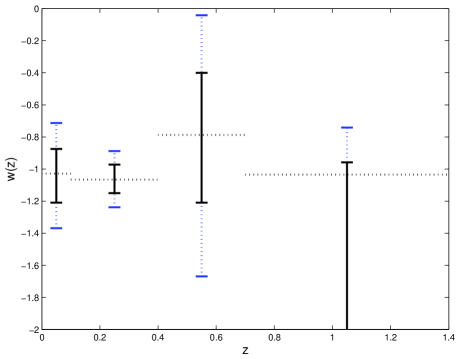
Figure 5: The $1\sigma$ and $2\sigma$ estimates of the four uncorrelated parameters $\mathcal{W}_{i}$.

Table 1: The marginalized $1\sigma$ errors for parameters constrained by the observational data

	$\chi^{2}$/DOF	$\Omega_{m}$	$\Omega_{k}$	$w_{0}\ (q_{1})$	$w_{a}\ (q_{2})$	AIC	BIC
$\Lambda$CDM	541.2/576	$0.272_{-0.011}^{+0.013}$	$0.002\pm 0.004$			545.2	553.9
DGP	561.6/576	$0.288_{-0.011}^{+0.015}$	$0.019\pm 0.005$			565.6	574.3
CPL	540.5/574	$0.265^{+0.019}_{-0.009}$	$0.008^{+0.005}_{-0.011}$	$-1.16_{-0.06}^{+0.26}$	$0.69^{+0.24}_{-1.41}$	548.5	565.9
JBP	540.6/574	$0.263^{+0.02}_{-0.01}$	$0.004\pm 0.006$	$-1.21_{-0.18}^{+0.32}$	$1.29^{+1.35}_{-2.33}$	548.6	566.0
Wetterich	540.4/574	$0.264\pm 0.013$	$0.009_{-0.005}^{+0.014}$	$-1.17^{+0.09}_{-0.23}$	$0.32_{-0.16}^{+0.46}$	548.4	565.8
$q_{1}-q_{2}$ model	542.6/576			$0.07\pm 0.11$	$-1.43\pm 0.09$	546.6	555.3
flat CPL	541.1/575	$0.267^{+0.019}_{-0.01}$		$-1.05_{-0.1}^{+0.17}$	$0.07^{+0.32}_{-0.88}$	547.1	560.2
flat JBP	541.0/575	$0.265^{+0.019}_{-0.011}$		$-1.08_{-0.19}^{+0.24}$	$0.32^{+1.01}_{-1.72}$	547.0	560.1
flat Wetterich	541.1/575	$0.266_{-0.015}^{+0.01}$		$-1.05^{+0.02}_{-0.16}$	$0.14\pm 0.1$	547.1	560.2

4 Conclusions

We summarize all the results in Table 1 and some results are shown in Figs. 1-5. By parametrizing the deceleration parameter $q(z)$, we find very strong evidence for the current acceleration. For the piecewise parametrization of $q(z)$, we find that $q(z)<0$ in the redshift range $0\leq z\la 0.6$, and $q(z)>0$ in the redshift range $z>0.8$ as shown in Fig. 3. So the Universe experiences accelerated expansion up to the redshift $z\sim 0.6$ and decelerated expansion at large redshift $z>0.8$. For the CPL, JBP and Wetterich models, we see from Fig. 1 that $\Lambda$CDM model is consistent with them, and this is further confirmed by the $Om$ diagnostic as shown in Fig. 2. The piecewise parametrization of $w(z)$ also confirms that $\Lambda$CDM model is consistent with current observations as shown in Fig. 5. The CPL, JBP and Wetterich models differ in the behaviour of $w(z)$ at high redshift; from Table 1 we see that all of them fit the observational data well, and $w(z)\la 0$ as seen in Fig. 1(a). So the current data is still unable to distinguish models with different behaviours of $w(z)$ at a high redshift. The number of parameters for $\Lambda$CDM and DGP models are the same, the difference between the best-fitting value of $\chi^{2}$ is $\Delta\chi^{2}=20.4$, so DGP model is excluded by the current data at more than $3\sigma$ level. The observational constraint on the growth index $\gamma$ is $\gamma=0.46^{+0.12}_{-0.08}$ for the DGP model which is more than $1\sigma$ away from the theoretical value $11/16$, and the growth index of $\Lambda$CDM model is $\gamma=0.56^{+0.14}_{-0.09}$ which is consistent with the theoretical value $6/11$. Our results also show that the Universe is almost flat. By using the prior $-5\leq\log|\Omega_{k}|\leq 0$, it was found that $-0.9\times 10^{-2}\leq\Omega_{k}\leq 0.01$ at 99% confidence level with the Bayesian model averaging method (Vardanyan, Trotta & Silk, 2011). In order to compare different models with different number of parameters, we usually apply Akaike Information Criterion (AIC) (Akaike, 1974). In terms of AIC, $\Lambda$CDM model is slightly preferred by the current data. Furthermore, to account for the effects of the number of data points and the number of parameters, Bayesian Information Criterion (BIC) (Schwarz, 1974) is used for model comparison. In terms of BIC, the $\Lambda$CDM model is again preferred by the current data. In addition to the approximate methods like AIC or BIC for model comparison, the Bayesian model comparison provides a better tool for model selection (Trotta, 2008).

Our results are based on the standard $\chi^{2}$ method which has some shortcomings (March et al., 2011), so March et al. (2011) presented the Bayesian hierarchical method to constrain the cosmological parameters and argued that the new method gives tighter constraint and outperforms the standard $\chi^{2}$ method.

References

- Akaike (1974) Akaike H., 1974, IEEE Trans. Auto. Control, 19, 716
- Amanullah et al. (2010) Amanullah R. et al., 2010, ApJ, 716, 712
- Ângela et al. (2008) da Ângela J. et al., 2008, MNRAS, 383, 565
- Schwarz (1974) Schwarz G., 1978, Ann. Stat., 5, 461
- Blake et al. (2010) Blake C. et al., 2010, MNRAS, 406, 803
- Cai, Su & Zhang (2010) Cai R. G., Su Q. P., Zhang H.-B., 2010, J. Cosm. Astropart. Phys., 04, 012
- Chevallier & Polarski (2001) Chevallier M., Polarski D., 2001, Int. J. Mod. Phys. D, 10, 213
- Clarkson, Cortês & Bassett (2007) Clarkson C., Cortês M., Bassett B., 2007, J. Cosm. Astropart. Phys., 08, 011
- Conley et al. (2008) Conley A. et al., 2008, ApJ, 681, 482
- Dossett et al. (2010) Dossett J., Ishak M., Moldenhauer J., Gong Y.G., Wang A., 2010, J. Cosm. Astropart. Phys., 04, 022
- Dvali, Gabadadze & Porrati (2000) Dvali G., Gabadadze G., Porrati, M., 2000, Phys. Lett. B, 485, 208
- Eisenstein & Hu (1998) Eisenstein D. J., Hu W., 1998, ApJ, 496, 605
- Eisenstein et al. (2005) Eisenstein D. J. et al., 2005, ApJ, 633, 560
- Gaztañaga, Miquel & Sánchez (2009a) Gaztañaga E., Miquel, R., Sánchez E., 2009a, Phys. Rev. Lett., 103, 091302
- Gaztañaga, Cabré & Hui (2009b) Gaztañaga E., Cabré A., Hui L., 2009b, MNRAS, 399, 1663
- Gong & Wang (2007) Gong Y. G., Wang, A., 2007, Phys. Rev. D, 75, 043520
- Gong (2008) Gong Y.G., 2008, Phys. Rev. D, 78, 123010
- Gong, Wu & Wang (2008) Gong Y. G., Wu Q., Wang A., 2008, ApJ, 681, 27
- Gong, Ishak & Wang (2009) Gong Y. G., Ishak M., Wang A., 2009, Phys. Rev. D, 80, 023002
- Gong et al. (2010a) Gong Y. G., Cai R. G., Chen Y, Zhu Z. H., 2010a, J. Cosm. Astropart. Phys., 01, 019
- Gong, Wang & Cai (2010b) Gong Y. G., Wang B., Cai R.G., 2010b, J. Cosm. Astropart. Phys., 04, 019
- Guzzo et al. (2008) Guzzo L. et al., 2008, Nature, 451, 541
- Hicken et al. (2009) Hicken M., Wood-Vasey W. M., Blondin S., Challis P., Jha S., Kelly P. L., Rest A., Kirshner R. P., 2009, ApJ, 700, 1097
- Hu & Sugiyama (1996) Hu W., Sugiyama N., 1996, ApJ, 471, 542
- Huang et al. (2009) Huang Q. G., Li M., Li X. D., Wang S., 2009, Phys. Rev. D, 80, 083515
- Huterer & Cooray (2005) Huterer D., Cooray A., 2005, Phys. Rev. D, 71, 023506
- Jassal, Bagla & Padmanabhan (2005) Jassal H. K., Bagla J. S., Padmanabhan T., 2005, MNRAS, 356, L11
- Kessler et al. (2010) Kessler R. et al., 2010, ApJS, 185, 32
- Komatsu et al. (2011) Komatsu E. et al., 2011, ApJS, 192, 18
- Kowalski et al. (2008) Kowalski M. et al., 2008, ApJ, 686, 749
- Lampeitl et al. (2009) Lampeitl H. et al., 2009, MNRAS, 401, 2331
- Lewis & Bridle (2002) Lewis A., Bridle S., 2002, Phys. Rev. D, 66, 103511
- Linder (2003) Linder E. V., 2003, Phys. Rev. Lett., 90, 091301
- March et al. (2011) March M. C., Trotta R., Berkes P., Starkman G. D., Vaudrevange P. M., 2011, arXiv: 1102.3237
- McDonald et al. (2005) McDonald P. et al., 2005, ApJ, 635, 761
- Pan et al. (2010) Pan N.N., Gong Y.G., Chen Y., Zhu Z.H., 2010, Class. Quantum Grav., 27, 155015
- Percival et al. (2007) Percival W. J., Cole S., Eisenstein D. J., Nichol R. C., Peacock J. A., Pope A. C., Szalay A. S., 2007, MNRAS, 381, 1053
- Percival et al. (2010) Percival W. J. et al., 2010, MNRAS, 401, 2148
- Perlmutter et al. (1999) Perlmutter S. et al., 1999, ApJ, 517, 565
- Riess et al. (1998) Riess A. G. et al., 1998, AJ, 116, 1009
- Riess et al. (2009) Riess A. G. et al., 2009, ApJ, 699, 539
- Ross et al. (2007) Ross N.P. et al., 2007, MNRAS, 381, 573
- Sahni, Shafieloo & Starobinsky (2008) Sahni V., Shafieloo A., Starobinsky A. A., 2008, Phys. Rev. D, 78, 103502
- Serra et al. (2009) Serra P., Cooray A., Holz D. E., Melchiorri A., Pandolfi S., Sarkar D., 2009, Phys. Rev. D, 80, 121302
- Shafieloo, Sahni & Starobinsky (2009) Shafieloo A., Sahni V., Starobinsky, A. A., 2009, Phys. Rev. D, 80, 101301
- Sollerman et al. (2009) Sollerman J. et al., 2009, ApJ, 703, 1374
- Stern et al. (2010) Stern D., Jimenez R., Verde L., Kamionkowski M., Stanford S. A., 2010, J. Cosm. Astropart. Phys., 02, 008
- Tegmark el al. (2006) Tegmark M. el al., 2006, Phys. Rev. D, 74, 123507
- Trotta (2008) Trotta R., 2008, Contemporary Phys., 49, 71
- Vardanyan, Trotta & Silk (2011) Vardanyan M., Trotta R., Silk J., 2011, MNRAS, 413, L91.
- Viel, Haehnelt & Springel (2004) Viel M., Haehnelt M.G., Springel V., 2004, MNRAS, 354, 684
- Viel, Haehnelt & Springel (2006) Viel M., Haehnelt M.G., Springel V., 2006, MNRAS, 365, 231
- Wetterich (2004) Wetterich C., 2004, Phys. Lett. B, 594, 17