New Horizons in Gravity:
The Trace Anomaly, Dark Energy & Condensate Stars

Abstract

General Relativity receives quantum corrections relevant at macroscopic distance scales and near event horizons. These arise from the conformal scalar degrees of freedom in the extended effective field theory of gravity generated by the trace anomaly of massless quantum fields in curved space. The origin of these conformal scalar degrees of freedom as massless poles in two-particle intermediate states of anomalous amplitudes in flat space is exposed. These are non-local quantum pair correlated states, not present in the classical theory. At event horizons the conformal anomaly scalar degrees of freedom can have macroscopically large effects on the geometry, potentially removing the classical event horizon of black hole and cosmological spacetimes, replacing them with a quantum boundary layer where the effective value of the gravitational vacuum energy density can change. In the effective theory, the cosmological term becomes a dynamical condensate, whose value depends upon boundary conditions near the horizon. In the conformal phase where the anomaly induced fluctutations dominate, and the condensate dissolves, the effective cosmological “constant” is a running coupling which has an infrared stable fixed point at zero. By taking a positive value in the interior of a fully collapsed star, the effective cosmological term removes any singularity, replacing it with a smooth dark energy interior. The resulting gravitational condensate star configuration resolves all black hole paradoxes, and provides a testable alternative to black holes as the final state of complete gravitational collapse. The observed dark energy of our universe likewise may be a macroscopic finite size effect whose value depends not on microphysics but on the cosmological horizon scale. The physical arguments and detailed calculations involving the trace anomaly effective action, auxiliary scalar fields and stress tensor in various situations and backgrounds supporting this hypothesis are reviewed. Originally delivered as a series of lectures at the Kraków School, the paper is pedagogical in style, and wide ranging in scope, collecting and presenting a broad spectrum of results on black holes, the trace anomaly, and quantum effects in cosmology.

I Introduction: Gravitation and Quantum Theory

Although it has been clear for nearly a century that quantum principles govern the microscopic domain of atomic, nuclear and particle physics, and certainly the Standard Model of Strong & Electroweak interactions is a fully quantum theory of matter, gravitational phenomena are still treated as completely classical in Einstein’s General Relativity. Perhaps just as significant as this formal gap between gravitation and quantum principles, most of our intuitions about gravity remain essentially classical, particularly in the macroscopic domain. Although it is generally agreed that at the fundamental microscopic Planck scale, a theory of gravitational interactions must come to terms with the quantum aspects of matter and even of spacetime itself, it is usually assumed that quantum effects are negligible on the scale of macroscopic phenomena, at astrophysical or cosmological distance scales, where classical General Relativity (GR) is presumed to hold full sway.

In non-gravitational physics quantum effects are present on a wide range of scales in a variety of ways, some of them striking, others more subtle and less immediately appreciated. Semi-conductors, superfluids, superconductors and atomic Bose-Einstein condensates are unmistakable macroscopic manifestations of an underlying quantum world. On astrophysical scales, the degeneracy pressure of fermions, which at first seemed an esoteric feature of quantum statistics is now fully accepted as the basis for the stability of such macroscopic objects as white dwarves and neutron stars, both of which are ubiquitous throughout the universe. As a posteriori consequences of quantum statistics one may note the periodic table, the foundations of chemistry itself and hence of biological processes, which being familiar in ordinary experience seem far less exotic than neutron stars or superfluidity. However chemical bonding, the structure and function of hemoglobin and DNA in the human body, and the overall stability of matter itself at ordinary temperatures and densities are every bit a consequence of quantum principles as a sample of superfluid ⁴He climbing up the walls of its dewar.

It was not only in the microscopic world of the atom but experiments on macroscopic matter and the puzzles they generated for classical mechanics, such as the ultraviolet problem of blackbody radiation and the specific heat of solids, that led to the development of quantum mechanics Planck ; EincV . Since quantum effects play a role in the properties of bulk matter and macroscopic phenomena in most every other area of physics, there is no reason why gravity, which couples to the energy content of quantum matter at all scales, should be immune from quantum effects on macroscopic scales.

If the effects and predictions of a quantum theory of gravity can be tested only at Planck lengths or energies, the quest for such a theory would be mostly academic, an exercise better left for future generations possessing more complete and accurate information about the ultra microscopic world. Thus the important questions at the outset are: Are quantum effects anywhere relevant or distinguishable in the macroscopic domain of gravitational phenomena? And if so, can one say anything reliable about macroscopic quantum effects in gravity, without necessarily possessing a complete, fundamental and well tested theory valid down to the microscopic Planck scale?

There are two problems at the forefront of current research where there are indications that quantum effects may play a decisive role in gravitational physics at macroscopic distance scales. The first of these is that of ultimate gravitational collapse, presumed in classical GR to lead a singularity of spacetime called a black hole, which generates a number of theoretical paradoxes and challenges for quantum theory. The second problem of great current interest is the apparent existence of cosmological dark energy, which is causing the expansion of the universe to accelerate, and which has the same equation of state $p=-\rho$ as that of the quantum vacuum itself.

Both of these problems are at the intersection of gravitation and quantum theory at macroscopic length scales. In both cases an approximate or effective theory of quantum effects in gravity far from the Planck scale should be the appropriate and only framework necessary. In these notes, such an effective field theory (EFT) framework is developed according to the same general principles now widely recognized in other areas of physics. The essential technical tools involve the use of relativistic quantum field theory in curved spacetime, and the key ingredient of our analysis is the conformal or trace anomaly of the stress-energy-momentum tensor $T^{a}_{\ b}$ of massless fields, a quantum effect with low energy implications.

Within this essentially semi-classical EFT framework, the principal qualitative result is that Einstein’s General Relativity can and does receive quantum corrections from the effects of the trace anomaly which are significant and in certain circumstances may even dominate at macroscopic distance scales, much larger than the Planck scale. No assumptions about the extreme short distance degrees of freedom or the precise nature of fundamental interactions at that scale will be used or needed. Instead our analysis will rely only upon the assumption that the Principle of Equivalence in the form of coordinate invariance of the effective action of a metric theory of gravity under smooth coordinate transformations applies in the quantum theory at sufficiently low energy scales far below the Planck scale. With this moderate theoretical input, and without invoking unknown or esoteric physics beyond the Standard Model, we shall investigate the macroscopic effects of the quantum conformal anomaly on gravitational systems at the astrophysical scale of the event horizon of the collapse of massive stars, and on the very largest Hubble scale of the visible universe itself.

II The Challenge of Black Holes

The first problem in which classical General Relativity is challenged by quantum theory is in the physics of black holes. Before discussing quantum effects, let us review the standard classical theory of the gravitational collapse of massive stars.

A normal main sequence star sustains itself by nuclear fusion of hydrogen into helium. The star itself formed when enough predominantly hydrogen gas collapsed to a high enough density for nuclear fusion reactions to occur. The energy generated by the fusion of H into He nuclei generates heat and pressure, which supports the star against further gravitational collapse. A main sequence star remains in this stable steady state, producing radiant energy for typically several billions of years, depending upon its mass. Eventually, the hydrogen is exhausted, and the star goes through a sequence of less exothermic nuclear reactions, fusing nuclei of heavier and heavier elements to extract energy from the difference in rest masses. Since iron is the most stable nucleus, this process eventually exhausts all the available sources of nuclear fusion energy. At that point the star can no longer sustain itself against the force of gravity, and its matter must resume gravitational collapse upon itself.

Classically, nothing can halt this collapse. However, quantum matter obeys quantum statistics. Because of Fermi-Dirac statistics, if the mass of the star is not too great, and it has cooled sufficiently, a new stable configuration, a white dwarf star held up by its quantum degeneracy pressure can be formed. In other cases, the collapse of the outer envelope onto the Fe core produces a violent explosion, a stellar nova or supernova, in which prodigious amounts of mass and energy are ejected. This leaves behind a even more compact object in which the electrons and protons are forced under high pressure to become neutrons. A neutron star, sustained against further collapse by the quantum degeneracy pressure of neutron matter, rotating very rapidly at nuclear densities and beaming out radiation guided by its strong magnetic fields may be observed by astronomers as a pulsar.

If the mass of the stellar remnant core exceeds a certain value, called the Tolman-Oppenheimer-Volkoff (TOV) limit of $1.5M_{\odot}$ to $3.2M_{\odot}$ (depending upon the eq. of state of dense nuclear matter, which is not very accurately known), not even the neutron degeneracy pressure is enough to prevent final and inexorable collapse due to gravity TOV . Since we have no direct observations of these final stages of complete gravitational collapse, it is here that the reliance upon Einstein’s theory of General Relativity becomes critical, and the discussion takes on a decidely more mathematical flavor.

II.1 Black Holes in Classical General Relativity

Just a year after the publication of the field equations of General Relativity (GR), K. Schwarzschild found a simple, static, spherically symmetric solution of those equations, with the line element Schw ,

$$ds^{2}=-f(r)\,d\tau^{2}+\frac{dr^{2}}{h(r)}+r^{2}\left(d\theta^{2}+\sin^{2}\theta\,d\phi^{2}\right)\,,$$ (1)

where in this case the two functions of $r$ are equal:

$$f(r)=h(r)=1-\frac{2GM}{c^{2}r}\,.$$ (2)

This Schwarzschild solution to the vacuum Einstein’s equations, with vanishing Ricci tensor $R^{a}_{\ b}=0$ and stress tensor $T^{a}_{\ b}=0$ for all $r>0$ describes an isolated, non-rotating object of total mass $M$. In that sense it is the gravitational equivalent of the Coulomb solution,

$$\phi=\frac{e}{r}$$ (3)

for the electrostatic potential of an isolated, static charge $e$ in Maxwell’s theory of electromagnetism. Just as in the Coulomb case, the Schwarzschild solution has a singularity at the origin of the spherical coordinates at $r=0$, where the gauge invariant field strengths (measured in gravity by the Riemann curvature tensor and its contractions) diverge, and there is a delta function source.

In classical electromagnetism at the finite scale of the classical electron radius, $r_{{}_{c}}=e^{2}/mc^{2}$, where the electrostatic self-energy becomes comparable to the rest mass energy, some deviation from the simple picture of a structureless point particle is to be expected. In quantum electromagnetism (QED) the classical linear divergence of (3) is softened somewhat into a logarithmic ultraviolet divergence of the self-energy of a charged Dirac particle. This logarithmically divergent self-energy is absorbed into a renormalization of its total observable mass. However already at the larger scale of the electron Compton wavelength $\hbar/mc>r_{{}_{c}}$, the single electron description has to be replaced by the many body description of a quantum field theory with vacuum polarization effects. Hence the pointlike singularity and linear divergence of the classical Coulomb potential (3) is not present in the more accurate many body quantum theory.

Apart from the singularity at $r=0$, analogous to (3) the Schwarzschld line element also possesses another kind of mathematical singularity at the finite Schwarzschild radius,

$$r_{{}_{S}}\equiv\frac{2GM}{c^{2}}\simeq 2.953\left(\frac{M}{M_{\odot}}\right)\,{\rm km}\,,$$ (4)

where the function $f(r)=h(r)$ vanishes. This macroscopic radius is the location of the Schwarzschild event horizon, the locus of points which defines the sphere dividing the exterior region from the interior region. It is the analog of the classical radius $r_{{}_{c}}$ where the Newtonian gravitational self-energy $GM^{2}/r$ becomes comparable to the total rest mass energy $Mc^{2}$. Thus $r_{{}_{S}}$ is the length scale at which some substructure should be expected.

Classical General Relativity does not give much hint of this substructure. Instead, the change of sign of the functions $f(r),h(r)$ for $r<r_{{}_{S}}$ in (2) indicates that for the interior region $t$ becomes a spacelike variable, while $r$ becomes timelike. Hence any radiation, even a light ray emanating from a point in the interior cannot propagate outward and is drawn inexorably toward the singularity at $r=0$, giving rise to the popular name black hole.

If the Schwarzschild solution (1)-(2) for $r<r_{{}_{S}}$ is taken seriously, the singularity at $r=0$ is present in Einstein’s theory for any mass $M>0$, including the certainly macroscopic mass of a collapsed star with the mass of the sun, $M_{\odot}\simeq 2\times 10^{33}$ gm. or even that of supermassive objects with masses $10^{6}$ to $10^{9}M_{\odot}$. The collapse of such enormous quantities of matter with vastly more degrees of freedom than that of a single electron to a single mathematical point at $r=0$ certainly presents a challenge to the imagination, and one that it seems Einstein himself sought arguments to avoid Ein . The situation is scarcely more acceptable if the singularity is removed only by the intervention of quantum effects at the extremely tiny Planck length $(G\hbar/c^{3})^{\frac{1}{2}}\sim 1.6\times 10^{-33}$ cm.

A light wave emitted from any $r>r_{{}_{S}}$ with local frequency $\omega_{loc}$ outward towards infinity is redshifted according to the redshift relation,

$$\omega_{\infty}=\omega_{loc}\,f^{\frac{1}{2}}=\omega_{loc}\sqrt{1-\frac{r_{{}_{S}}}{r}}\,,$$ (5)

showing that a light wave emitted at the horizon becomes redshifted to zero frequency and cannot propagate outward at all. Conversely and equivalently, a light wave with the finite frequency $\omega=\omega_{\infty}$ far from the black hole is blueshifted to an infinite local frequency at the horizon. This gravitational redshift/blueshift is purely a kinematic consequence of the classical time dilation effect of a gravitational field, which has been tested in a number of experiments MTW ; WeinG ; Will . The event horizon is therefore a kind of critical surface for the propagation of light rays, and hence all other matter interactions.

Unlike the central singularity at $r=0$, the scalar invariant quantities that can be constructed from the contractions of the Riemann curvature tensor remain finite as $r\rightarrow r_{{}_{s}}$. Thus the fully contracted quadratic Riemann invariant

$$R^{abcd}R_{abcd}=\frac{12r_{{}_{S}}^{2}}{r^{6}}\,,$$ (6)

which diverges at the origin remains finite at $r=r_{{}_{S}}$. Moreover, although the time for an infalling particle to reach the horizon is infinite for any observer remaining fixed outside the horizon, the proper time measured by the particle itself during its infall remains finite as $r\rightarrow r_{{}_{s}}$ MTW ; WeinG . Thus despite the singularity of the Schwarzschild coordinates at $r=r_{{}_{S}}$, physics must continue onto smaller values of $r$ in the interior region. Since the line element (1) is again non-singular for $0<r<r_{{}_{S}}$, and in the absence of clear evidence to the contrary, the most straightforward possibility would seem to be to assume that this non-singular vacuum interior (up to the origin or at least some extreme microscopic scale much less than $r_{{}_{S}}$) can be matched smoothly to the non-singular exterior Schwarzschild solution.

This matching was achieved by the coordinate transformations and analytic continuation of the Schwarzschild solution found by Kruskal and Szekeres KrusSz . The Kruskal maximal analytic extension of the Schwarzschild geometry is pictured in the Carter-Penrose conformal diagram, Fig. 1.

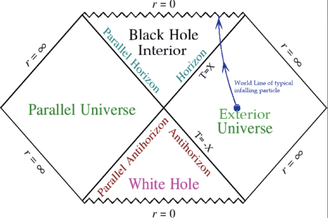
Figure 1: The Carter-Penrose conformal diagram of the maximal Kruskal analytic extension of the Schwarzschild geometry. Radial light rays are represented in this diagram as $45^{\circ}$ lines. The angular coordinates $\theta,\phi$ are suppressed.

The analytic extension of the Schwarzschild geometry relies on finding a judicious change of the time and radial coordinates $(t,r)$ of (1) to new ones $(T,X)$, which are regular on the horizon, and therefore can be used to describe the local geometry there without singularities. Explicitly, for $r>r_{{}_{S}}$ this coordinate transformation to Kruskal-Szekeres coordinates $(T,X)$ is given by

$$T=\left(\frac{r}{r_{{}_{S}}}-1\right)^{\frac{1}{2}}\,e^{r/2r_{{}_{S}}}\,\sinh\left(\frac{ct}{2r_{{}_{S}}}\right)\,,$$ (7a)

$$X=\left(\frac{r}{r_{{}_{S}}}-1\right)^{\frac{1}{2}}\,e^{r/2r_{{}_{S}}}\,\cosh\left(\frac{ct}{2r_{{}_{S}}}\right)\,.$$ (7b)

The inverse transformation is

$$t=\frac{2r_{{}_{S}}}{c}\tanh^{-1}\left(\frac{T}{X}\right)=\frac{r_{{}_{S}}}{c}\,\ln\left(\frac{X+T}{X-T}\right)\,$$ (8a)

$$\hskip 28.45274pt\left(\frac{r}{r_{{}_{S}}}-1\right)\,e^{r/r_{{}_{S}}}=X^{2}-T^{2}\,.$$ (8b)

In the new $(T,X)$ coordinates, the Schwarzschild line element (2) becomes

$$ds^{2}=\frac{4r_{{}_{S}}^{3}}{r}\,e^{r/2r_{{}_{S}}}\,(-dT^{2}+dX^{2})+r^{2}d\Omega^{2}\,,$$ (9)

where $r$ is to be regarded as the function of $(T,X)$ given implicitly by (8b), and $d\Omega^{2}=d\theta^{2}+\sin^{2}\theta\,d\phi^{2}$ is the usual spherical line element on ${\mathbb{S}}^{2}$.

In these Kruskal-Szekeres coordinates, the event horizon at $r=r_{{}_{S}}$ is seen actually to be comprised of two distinct null surfaces, the future and past horizons for $T=\pm X$, respectively. The entire exterior region $r>r_{{}_{S}}$ is mapped into the region $X>|T|\geq 0$ of the $(X,T)$ plane. The $X=+T$ boundary of this region gives the coordinates of a particle trajectory infalling into the black hole, a depicted in Fig. 1, whereas the $X=-T$ boundary corresponds to the time reversed coordinates of a particle trajectory outgoing from a white hole. The time reversed case must be present mathematically because of the second order nature of Einstein’s eqs., and the static solution (1) which admits the time reversal symmetry $t\rightarrow-t$ and $T\rightarrow-T$. Whether or not this time reversed white hole case corresponds to any real macroscopic body is of course another question.

Since the Schwarzschild line element in Kruskal-Szekeres coordinates (9) is completely regular at $T=\pm X$, one can equally well consider the extension of the coordinates to the interior regions, $T>X>0$ and $T<-X<0$, into the black hole and white hole interior regions at the top and bottom of Fig. 1, at least as far and until the true curvature singularity at $r=0$ is reached. Inspection of (8) shows that this implies an analytic continuation of the original Schwarzschild $(t,r)$ coordinates around a logarithmic branch cut to complex values. The relation of the $(T,X)$ coordinates to the original $(t,r)$ coordinates is singular at $r=r_{{}_{S}}$, although the $(T,X)$ coordinates themselves are regular at $T=\pm X$. Similarly, by a further complex analytic continuation, one can continue to the parallel exterior region on the left of Fig. 1 with $X<-|T|\leq 0$. Thus, by the relatively simple but singular change of coordinates (7)-(8), we seem to have reached the conclusion that the simplest static spherically symmetric Schwarzschild solution to the vacuum Einstein’s equations predicts the existence not only of a true singularity at $r=0$ but also of an entirely separate and macroscopically large, asymptotically flat region in addition to the original one.

Of course, one is free to assert that the white hole interior region and the parallel asymptotically flat universe do not exist, and excise them in a gravitational collapse from realistic initial conditions, replacing the excised region of Fig. 1 with the non-singular interior of a collapsing matter distribution. However, this is a matter of initial conditions, and nothing in the equations of General Relativity themselves forces us to do this. Dirac expressed skepticism of the interior Schwarzschild solution on physical grounds Dir .

The apparently unphysical features of the Schwarzschild solution appear as soon as we admit complex analytic continuation of singular coordinate transformations. Based on the Principle of Equivalence between gravitational and inertial mass, Einstein’s theory possesses general coordinate invariance under all regular and real transformations of coordinates. It is the appending to classical General Relativity of the much stronger mathematical hypothesis of complex analytic continuation through singular coordinate transformations that leads to the global aspects of the Schwarzschild solution which may be unrealized in Nature.

The point which is often left unstated is that the mathematical procedure of analytic continuation through the null hypersurface of an event horizon actually involves a physical assumption, namely that the stress-energy tensor $T^{a}_{\ b}$ is vanishing there. Even in the purely classical theory of General Relativity, the hyperbolic character of Einstein’s equations allows generically for stress-energy sources and hence metric discontinuities on the horizon which would violate this assumption. Additional physical information is necessary to determine what happens as the event horizon is approached, and the correct matching of interior to exterior geometry. What actually happens at the horizon is a matter of this correct physics, which may or may not be consistent with complex analytic continuation of coordinates (7)-(8).

The static Schwarzschild solution of an isolated uncharged mass was generalized to include electric charge by Reissner & Nordstrøm RN , and more interestingly for astrophysically realistic collapsed stars, to include rotation and angular momentum by Kerr Kerr . The complete analytic extensions of the Reissner-Nordstrøm and Kerr solutions were found as well BoyLinCar . The global properties of these analytic extensions are more complicated and arguably even more unphysical than in the Schwarzschild case. For slowly rotating black holes with angular momentum $J<GM^{2}/c$, there are an infinite number of black hole interior and asymptotically flat exterior regions, and closed timelike curves in the interior region(s), which violate causality on macroscopic distance scales HawEll . Again these apprently unphysical features appear in GR only if the mathematical hypothesis of complex analytic extension and continuation through real coordinate singularities are assumed. This analytic continuation is generally invalid if there are stress-tensor sources encountered at or before the breakdown of coordinates.

The Schwarzschild white hole and the analytic extension through the horizons also raises questions about macroscopic time reversibility. Once classical particles fall through the future event horizon, there is no way to retrieve them without violating causality, and something irreversible would seem to have occurred. This is somewhat troubling from the point of view of thermodynamics, since if matter disappears completely from view when it falls into a black hole, it carries any entropy it has in its internal states with it, and the entropy of the visible universe would apparently have decreased, violating the second law of thermodynamics,

$$\Delta S\geq 0\,,$$ (10)

which states that the total entropy of an isolated system must be a non-decreasing function of time in any spontaneous process.

At the same time the infall of matter into a black hole certainly increases its total energy. In the general black hole solution characterized by mass $M$, angular momentum $J$, and electric charge $Q$, one can define a quantity called the irreducible mass $M_{irr}$ by the relation,

$$M^{2}=\left(M_{irr}+\frac{Q^{2}}{4GM_{irr}}\right)^{2}+\frac{c^{2}J^{2}}{4G^{2}M_{irr}^{2}}\,,$$ (11)

or

$$M^{2}_{irr}=\frac{M^{2}}{2\ }-\frac{Q^{2}}{4G\ }+\frac{1}{2G}\,\left[G^{2}M^{4}-GM^{2}Q^{2}-c^{2}J^{2}\right]^{\frac{1}{2}}\,,$$ (12)

and show that in any classical process the irreducible mass can never decrease Mirr :

$$\Delta M^{2}_{irr}\geq 0\,.$$ (13)

Since one can also show that the irreducible mass is related to the geometrical area $A$ of the event horizon of the general Reissner-Nordstrøm-Kerr-Newman black hole via

$$A=\frac{16\pi G^{2}}{c^{4}}M^{2}_{irr}\,,$$ (14)

this theorem is equivalent to the statement that the horizon area is a non-decreasing function of time in any classical process Mirr ; HawA .

Simply by taking the differential form of (11) one obtains BCH

$$dE=dMc^{2}=\frac{c^{2}}{8\pi G}\,\kappa\,dA+\Omega\,dJ+\Phi\,dQ$$ (15)

which is just the differential form of Smarr’s formula for a Kerr-Newman rotating, electrically charged black hole, in which

$$\kappa=\frac{1}{M}\left[\frac{c^{4}}{4G}-\frac{4\pi^{2}G}{c^{4}A^{2}}\left(Q^{4}+4c^{2}J^{2}\right)\right],$$ (16a)

$$\Omega=\frac{4\pi J}{MA}\,,$$ (16b)

$$\Phi=\frac{Q}{M}\left[\frac{c^{2}}{2G}+\frac{2\pi Q^{2}}{Ac^{2}}\right]\,,$$ (16c)

$$A=\frac{4\pi G}{c^{4}}\,\left[2GM^{2}-Q^{2}+2\sqrt{G^{2}M^{4}-GM^{2}Q^{2}-c^{2}J^{2}}\right],$$ (16d)

are the horizon surface gravity, angular velocity, electrostatic potential and area respectively BCH ; Smarr . All dimensionful constants have been retained to emphasize that (15)-(16) are formulae derived from classical GR in which no $\hbar$ whatsoever appears. Notice also that the coefficient of $dA$ in (15), $c^{2}\kappa/8\pi G$ has both the form and dimensions of a surface tension.

The classical conservation of energy is expressed by the first law of black hole mechanics (15). The classical area theorem (13) naturally evokes a connection to entropy and the second law of thermodynamics (10). If horizon area (or more generally any monotonic function of it) could somehow be identified with entropy, and this entropy gain is greater than the entropy lost by matter or radiation falling into the hole, then the second law (10) would remain valid for the total or generalized entropy of matter plus black hole horizon area. The simplest possibility would seem to be if entropy is just proportional to area.

Motivated by these considerations, and as suggested by a series of thought experiments, Bekenstein proposed that the area of the horizon (14) should be proportional to the entropy of a black hole Bek . Since $A$ does not have the units of entropy, it is necessary to divide the area by another quantity with units of length squared before multiplying by Boltzmann’s constant $k_{{}_{B}}$, to obtain an entropy. However, classical General Relativity (without a cosmological term) contains no such quantity, $G/c^{2}$ being simply a conversion factor between mass and distance. Hence Bekenstein found it necessary for purely dimensional reasons to introduce Planck’s constant $\hbar$ into the discussion. Then there is a standard unit of length, namely the Planck length,

$$L_{Pl}=\sqrt{\frac{\hbar G}{c^{3}}}=1.616\times 10^{-33}\,{\rm cm.}$$ (17)

Bekenstein proposed that the entropy of a black hole should be

$$S_{{}_{BH}}=\gamma k_{{}_{B}}\frac{A}{L_{Pl}^{2}}\,,$$ (18)

with $\gamma$ a constant of order unity Bek . He showed that if such an entropy were assigned to a black hole, so that it is added to the entropy of matter, $S_{tot}=S_{m}+S_{{}_{BH}}$, then this total generalized entropy would plausibly always increase. In fact, this is not difficult at all, and the generalized second law $\Delta S_{tot}\geq 0$ is usually satisfied by a very wide margin, simply because the Planck length is so tiny, and the macroscopic area of a black hole measured in Planck units is so enormous. Hence even the small increase of mass and area caused by dropping into the black hole a modest amount of matter and concomitant loss of matter entropy $\Delta S_{m}<0$ is easily overwhelmed by a great increase in $S_{{}_{BH}}$, $\Delta S_{{}_{BH}}\gg|\Delta S_{m}|$, guaranteeing that the generalized total entropy increases: $\Delta S_{tot}>0$.

Since $\hbar$ has entered the assignment of entropy to a black hole horizon, the discussion can no longer be continued in purely classical terms, and we must discuss quantum effects in black hole geometries next. It is worth remarking that whereas Planck’s constant enters the thermodynamics of macroscopic quantum systems, such as the formulae for black body radiation, by normalizing the volume of the integral over phase space, no such interpretation is available for (18). Instead $\hbar$ has been used to form a new quantity $L_{Pl}$ with units of length, which we would ordinarily associate with the microscopic length scale at which strong quantum corrections to Einstein’s theory should become important. Why such a microscopic, fundamentally quantum length scale should be needed to determine the bulk thermodynamic entropy of a macroscopic object on the scale of kilometers where classical GR applies, and no large quantum corrections to GR are expected near the horizon, is far from clear.

II.2 Quantum Black Holes and Their Paradoxes

Since classically all matter is irretrievably drawn into a black hole, the idea that black holes can instead radiate energy seems quite counterintuitive. More remarkable still is Hawking’s argument that this radiation would necessarily be thermal radiation, with a temperature HawkT

$$T_{{}_{H}}=\frac{\hbar\kappa}{2\pi ck_{{}_{B}}}\ \,\stackrel{{\scriptstyle J=Q=0}}{{=}}\ \,\frac{\hbar c^{3}}{8\pi Gk_{{}_{B}}M}\,,$$ (19)

where the first equality is general, and the second equality applies only for a Schwarzschild black hole with $J=Q=0$. With the temperature inversely proportional to its mass assigned to a black hole by this formula, if we assume that the first law of thermodynamics in the form

$$dE=dMc^{2}=T_{{}_{H}}\,dS_{{}_{BH}}+\Omega\,dJ+\Phi\,dQ\,.$$ (20)

applies to black holes, then the coefficient $\gamma$ in (18) is fixed to be $1/4$. This formula is simple and appealing, and has been generally accepted since soon after Hawking’s paper first appeared. However, simultaneously and from the very beginning, a number of problems with this thermodynamic interpretation made their appearance as well.

The first curious feature of (20) is that $\hbar$ cancels out between $T_{{}_{H}}$ and $dS_{{}_{BH}}$. Of course, this is a necessary consequence of the fact that (20) is identical to the classical Smarr formula (15) in which $\hbar$ does not appear at all. The identification of $S_{{}_{BH}}$ with the entropy of a black hole is founded on the purely classical dynamics of Christodoulou’s area law (13), in which quantum mechanics played no part whatsoever. Clearly, multiplying and dividing by $\hbar$ does not necessarily make a classical relation a valid one in the quantum theory. On the other hand, the Hawking temperature (19) is a quantum spontaneous emission effect, analogous to the Schwinger pair creation effect in a strong electric field Schwinger which vanishes in the classical limit $\hbar\rightarrow 0$. Temperature, usually accepted as a classical concept has no apparent meaning for a black hole in the strictly classical limit, unless it is identically zero. As a consequence, if the identification of the classical area rescaled by $k_{{}_{B}}L_{Pl}^{-2}$ with entropy and the thermodynamic interpretation of (20) is to be generally valid in the quantum theory, then the classical limit $\hbar\rightarrow 0$ (with $M$ fixed) which yields an arbitrarily low Hawking temperature, assigns to the black hole an arbitrarily large entropy, completely unlike the zero temperature limit of any other cold quantum system.

Closely related to this paradoxical result is the fact, pointed out by Hawking himself HawkcV , that a temperature inversely proportional to the $M=E/c^{2}$ implies that the heat capacity of a Schwarzschild black hole,

$$\frac{dE}{dT_{{}_{H}}}=-\frac{8\pi Gk_{{}_{B}}M^{2}}{\hbar c}=-\frac{Mc^{2}}{T_{{}_{H}}}<0$$ (21)

is negative. In statistical mechanics the heat capacity of any system (at constant volume) is related to the energy fluctuations about its mean value $\langle E\rangle$ by

$$c_{{}_{V}}=\left(\frac{d\langle E\rangle}{dT}\right)_{{}_{V}}=\frac{1}{k_{{}_{B}}T^{2}}\,\Big{\langle}(E-\langle E\rangle)^{2}\Big{\rangle}>0\,.$$ (22)

If pressure or some other thermodynamic variable is held fixed there is an analogous formula. Hence on general grounds of quantum statistical mechanics, the heat capacity of any system in (stable) equilibrium must be positive. The positivity of the statistical average in (22) requires only the existence of a well defined stable ground state upon which the thermal equilibrium ensemble is defined, but is otherwise independent of the details of the system or its interactions.

In fact, it is easy to see that a black hole in thermal equilibrium with a heat bath of radiation at its own Hawking temperature $T=T_{{}_{H}}$ cannot be stable HawkcV . For if by a small thermal fluctuation it should absorb slightly more radiation in a short time interval than it emits, its mass would increase, $\Delta M>0$, and hence from (19) its temperature would decrease, $\Delta T<0$, so that it would now be cooler than its surroundings and be favored to absorb more energy from the heat bath than it emits in the next time step, decreasing its temperature further and driving it further from equilibrium. In this way a runaway process of the black hole growing to absorb all of the surrounding radiation in the heat bath would ensue. Likewise, if the original fluctuation has $\Delta M<0$, the temperature of the black hole would increase, $\Delta T>0$, so that it would now be hotter than its surroundings and favored to emit more energy than it absorbs from the heat bath in the next time step, increasing its temperature further. Then a runaway process toward hotter and hotter evaporation of all its mass to its surroundings would take place. In either case, the initial equilibrium is clearly unstable, and hence cannot be a candidate for the quantum ground state for the system. This is the physical reason why the positivity property of (22) is violated by the Hawking temperature (19). The instability has also been found from the negative eigenvalue of the fluctuation spectrum of a black hole in a box of (large enough) finite volume BHnegmode .

The time scale for this unstable runaway process to grow exponentially is the time scale for fluctuations away from the mean value of the Hawking flux, not the much longer time scale associated with the lifetime of the hole under continuous emission of that flux. This time scale for thermal fluctuations is easily estimated. It is the typical time between emissions of a single quantum with typical energy (at infinity) of $k_{{}_{B}}T$, of a source whose energy emission per unit area per unit time is of order $(k_{{}_{B}}T_{{}_{H}})^{4}/\hbar^{3}c^{2}$. Multiplying by the area of the hole $A\sim(GM)^{2}/c^{4}$, and dividing by the typical energy $k_{{}_{B}}T$, we find the average number of quanta emitted per unit time. The inverse of this, namely

$$\Delta t\sim\frac{1}{A}\frac{(\hbar c)^{3}}{(k_{{}_{B}}T_{{}_{H}})^{3}}\sim\frac{r_{{}_{S}}}{c}\sim 10^{-5}\left(\frac{M}{M_{\odot}}\right)\,{\rm sec}$$ (23)

is the typical time interval (as measured by a distant observer) between successive emissions of individual Hawking quanta (again as observed far from the black hole). This time scale is quite short: $10\ \mu$sec for a solar mass black hole. Any tendency for the system to become unstable would be expected to show up on this short a time scale, governing the fluctuations in the mean flux, which is of order of the collapse time itself and before a steady state flux could even be established. With the existence of a stable equilibrium in doubt, one may well question whether macroscopic equilibrium thermodynamic concepts such as temperature or entropy are applicable to black holes at all.

Another rather peculiar feature of the formula (18) for the entropy is that it is non-extensive, growing not like the volume of the system but its area. It is non-extensive in a second important respect. The fixing of $\gamma=1/4$ by (19) and (20) is independent of the number or kind of particle species. Normally, we would expect the entropy of a system to grow linearly with the number of distinct particle species it contains. For example, if the number of light neutrino species in the universe were doubled, the entropy in the primordial plasma would be doubled as well, because the available states of one species are independent of and orthogonal to the states of a second distinct species, and must be counted separately. The formula (18) with only fundamental constants and the pure number coefficient $\gamma=1/4$ does not seem to allow for this. ‘t Hooft found a way to compensate the number of species factor in the horizon “atmosphere,” but this configuration with matter or radiation densely concentrated near $r=r=r_{{}_{S}}$ is no longer then a Schwarzschild black hole tHatmos . It also remains singular at the origin.

Finally, let us state the obvious: a solution of any set of classical field equations is simply one particular configuration in the space of field configurations. As such, one would not usually associate any entropy with it. Matter sources to the field equations which have internal degrees of freedom may carry entropy of course, but a vacuum solution to the equations such as the Schwarzschild solution (1)-(2), with at most a singular point source at the origin would not ordinarily be expected to carry any entropy whatsoever. What “entropy” should one associate with the structureless classical Coulomb field (3)?

In this connection it may be worth pointing out that although the Coulomb field does not have an event horizon, there would still be an “information paradox” if we allowed charged matter to be attracted into (or emitted from) the Coulomb field singularity in (3) at $r=0$ and disappear from (or appear in) the visible universe. Such disappearance or appearance processes would clearly violate unitarity as well. In quantum theory we exclude such a possibility by restricting the Hilbert space of states to those with wave functions that are normalizable at the origin, so that no energy or momentum flux can either vanish or appear at the Coulomb singularity. Note that we impose this boundary condition at $r=0$ without any detailed knowledge of the extreme short distance structure of a charged particle in QED, confident that whatever it is, unitarity must be respected. In the case of black hole radiance by contrast, the positive Hawking energy flux at infinity must be balanced by a compensating flux down the hole and eventually into the singularity at $r=0$, which makes clear why problems with unitarity and loss of information must result from such a flux. Boundary conditions on the horizon have consequences for the behavior of the fluctuations at both the singularity and at infinity. As even the example of scattering off the Coulomb potential shows, these boundary conditions require physical input. Unphysical boundary conditions can easily lead to unphysical behavior.

Returning to the entropy (18), it is instructive to evaluate $S_{{}_{BH}}$ for typical astrophysical black holes. Taking again as our unit of mass the mass of the sun, $M_{\odot}\simeq 2\times 10^{33}$ gm., we have

$$S_{{}_{BH}}\simeq 1.050\times 10^{77}\,k_{{}_{B}}\,\left(\frac{M}{M_{\odot}}\right)^{2}\,.$$ (24)

This is truly an enormous entropy. For comparison, we may estimate the entropy of the sun as it is, a hydrogen burning main sequence star, whose entropy is given to good accuracy by the entropy of a non-relativistic perfect fluid. This is of the order $Nk_{{}_{B}}$ where $N$ is the number of nucleons in the sun $N\sim M_{\odot}/m_{{}_{N}}\sim 10^{57}$, times a logarithmic function of the density and temperature profile which may be estimated to be of the order of $20$ for the sun. Hence the entropy of the sun is roughly

$$S_{\odot}\sim 2\times 10^{58}\,k_{{}_{B}}\,,$$ (25)

or nearly $19$ orders of magnitude smaller than (24).

A simple scaling argument that the entropy of any gravitationally bound object with the mass of the sun cannot be much more than (25) can be made as follows. The entropy of a relativistic gas at temperature $T$ in equilibrium in a box of volume $V$ is of order $VT^{3}$. The total energy is of order $VT^{4}$. Eliminating $T$ from these relations gives $S\sim V^{\frac{1}{4}}E^{\frac{3}{4}}$. For a relativistic bound system the energy $E\sim Mc^{2}$ while the volume is of order $r_{{}_{S}}^{3}\sim(GM/c^{2})^{3}$. Hence $S\sim(\sqrt{G}M)^{\frac{3}{2}}$. Keeping track of $k_{{}_{B}}$, $\hbar$ and $c$ in this estimate gives

$$S\sim k_{{}_{B}}\left(\frac{M}{M_{Pl}}\right)^{\frac{3}{2}}\sim 10^{57}\,k_{{}_{B}}\left(\frac{M}{M_{\odot}}\right)^{\frac{3}{2}}\,,$$ (26)

where $M_{Pl}=\sqrt{\hbar c/G}=2.176\times 10^{-5}$ gm. If there are $\nu$ species of relativistic particles in the object then this estimate should be multiplied by $\nu^{\frac{1}{4}}$. This estimate applies to the entropy of relativistic radiation within the body, and is lower than (25) because the radiation pressure in the sun is small compared to the non-relativistic fluid pressure. However, the entropy from the relativistic radiation pressure (26) grows with the $3/2$ power of the mass, whereas the non-relativistic fluid entropy (25) grows only linearly with $M$. For stars with masses greater than about $50M_{\odot}$ which are hot enough for their pressure to be dominated by the photons’ $T^{4}$ radiation pressure, (26) indeed gives the correct order of magnitude estimate of such a star’s entropy at a few times $10^{59}k_{{}_{B}}$ ZelNov . In order to have such an entropy, the temperature of the star must be of order $E/S\sim 10$ MeV or $10^{11}\,{}^{\circ}$K, while the Hawking temperature (19) for the same $50M_{\odot}$ black hole is a very, very cold $10^{-9}\,{}^{\circ}$K. It is difficult to see how the entropy of the black hole could be a factor of $10^{20}$ larger while its temperature is a factor of $10^{20}$ lower than a relativistic star of the same mass.

The point is that even for the extreme relativistic fluid the entropy (26) for a gravitationally bound system in thermal equilibrium (in which entropy is always maximized) grows only like the $3/2$ power of the mass, and hence will always be much less than (24), proportional to $M^{2}$ for very massive objects. Moreover the discrepant factor between (24) and (26) is of order $(M/M_{Pl})^{\frac{1}{2}}\simeq 10^{19}(M/M_{\odot})^{\frac{1}{2}}$, no matter what the non-black hole progenitor of the black hole is. Since the formula (24) makes no reference to how the black hole was formed, and a black hole may always be theoretically idealized as forming from an adiabatic collapse process, which keeps the entropy constant, (24) states that this entropy must suddenly jump by a factor of order $10^{19}$ for a solar mass black hole at the instant the horizon forms. When Boltzmann’s formula,

$$S=k_{{}_{B}}\ln W(E)$$ (27)

is recalled, relating the entropy to the total number of microstates in the system $W(E)$ at the fixed energy $E$, we see that the number of such microstates of a black hole satisfying (24) must jump by $\exp(10^{19})$ at that instant at which the event horizon is reached, a truly staggering proposition.

This tremendous mismatch between the number of microstates of a black hole inferred from $S_{{}_{BH}}$ and that of any conceivable physical non-black hole progenitor is one form of the information paradox. Another form of the paradox is that since black holes are supposed to radiate thermally at temperature $T_{{}_{H}}$ up until their very last stages, when their mass falls to a value of order $M_{Pl}$, there would seem to be no way to recover all the information apparently lost in the black hole formation and evaporation process. This difficulty with $S_{{}_{BH}}$ is so severe that it led Hawking to speculate that perhaps even the quantum mechanical unitary law of evolution of pure states into pure states would have to be violated by black hole physics Hawkunit . Although this speculation has currently fallen into disfavor Hawnew , it is still far from clear what the missing microstates of an uncharged black hole are, and how exactly unitarity can be preserved in the Hawking evaporation process if (19) and (24) are correct.

For all of these reasons the thermodynamic interpretation of (20) remains problematic in quantum theory. On the other hand, if the $\hbar$ is cancelled and one simply returns to the differential Smarr relation (15), derived from classical GR, these difficulties immediately vanish. One would only be left to explain the relationship of surface gravity $\kappa$ to surface tension. In Refs. gstar ; PNAS and Sec. VII a possible resolution is proposed in which area is not entropy at all but indeed the area of a physical surface and the surface gravity can be related to the surface tension of this surface.

Although the thermodynamic interpretation of (20) and (24), leads to myriad difficulties, it has been essentially universally assumed, and great ingenuity has been devoted to postulating the new physics of some kind which would be needed to account for the vast number of microstates in the interior of a black hole required by (24). It is not possible to do justice to the various approaches in detail here. Curiously the multitude of approaches all seem to give the same answer, despite the fact that the states they are counting are very different Car . Of course, any theory that reduces to Einstein’s theory in an appropriate limit will conserve energy and obey the first law of thermodynamics. If the effective action of the theory reduces to the Einstein-Hilbert action then the logarithm of its generating functional $Z$ should produce the entropy (24), suggesting that these formal results are actually a feature of the classical theory, embodied in the Smarr formula (15), and independent of the model used or microstates counted.

The lines of research involving exotic internal constituents to obtain $S_{{}_{BH}}$ are all the more remarkable when one recalls where we began, with the classical GR expectation that all one has to do is change coordinates as in (7) to see that “nothing happens” at the event horizon to a particle falling through. If the horizon is really just a harmless coordinate singularity–the very assumption underlying the arguments leading to the Hawking temperature, and hence the entropy (24), how can the semi-classical assumption of no energy or stresses, and analyticity and regularity at the geometry at the horizon with no substructure in the interior then lead to the diametrically opposite conclusion of exotic new physics, with $\exp(10^{19})$ additional microstates, and perhaps the radical alteration of classical spacetime itself the instant the horizon is reached?

Counting the microstates hiding in electrically charged black holes in string theory or other models also leave unanswered the question of how a presumably well-defined quantum theory with a stable ground state (which always has a positive heat capacity) could ever yield the negative heat capacity (21) of the original, uncharged Schwarzschild black hole in $3+1$ dimensions.

Another line of thought has attempted to identify the entropy (24) with quantum entanglement entropy BKLS ; FroFur ; IsrBHT . This is the entropy that results when a quantum system is divided into two spatial partitions and one sums over the microstates of one of the partitions, forming a mixed state density matrix from a pure state wave functional even at zero temperature. This has the attractive feature that on general grounds it is proportional to the area of the surface at which the two partitions are in contact. It has the unattractive feature that the coefficient of the area law in quantum field theory is infinite. The reason for this ultraviolet divergence is the same as the reason for the area law itself, namely that the largest contribution to the entanglement entropy comes from the ultraviolet components of the wave functional within a vanishingly thin layer near the surface. If this divergence is cut off at a length scale of the order of $L_{Pl}$, a large but finite entropy of order of (18) is obtained FroFur .

Counting these states at very high frequencies as contributing to the entropy is sensible only if those states are occupied. In quantum statistical mechanics the unoccupied states at arbitrarily high energies, no matter how many of them, do not contribute to the thermodynamic entropy of the system. In the black hole case, the standard classical assumption of the horizon as a harmless coordinate singularity and the Hawking-Unruh state corresponding to this classical assumption (discussed in more detail in the next section) treats these high frequency states as unoccupied vacuum states with respect to a locally regular coordinate freely falling system at the horizon, such as (7). Hence it is difficult to see why they should be counted as contributing to the entropy. If on the contrary one treats these modes as occupied with respect to the singular static frame (1), then it is difficult to see why their mean energy-momentum or fluctuations in $\langle T^{a}_{\ b}\rangle$ should be negligible near the horizon. Since the Hawking thermal flux originates as radiation closer and closer to $r_{{}_{S}}$ with arbitrarily high frequencies at late times, if these states are occupied it is also difficult to see why any cutoff at the Planck scale or otherwise should be imposed to compute the entanglement entropy.

The attempt to count microstates near the horizon to account for the black hole entropy associated with the Hawking effect brings us face to face with questions about the structure and meaning of the “vacuum” itself at trans-Planckian frequencies. One way or another some physical input is needed to determine the precise boundary conditions on the near horizon modes upon which the entire set of results and physical consequences for macroscopic black hole physics hinge. At the horizon the classical supposition that nothing happens at a coordinate singularity is in tension with the behavior and assumptions of quantum field theory (in a fixed background) at very high frequencies. This tension is the source of the paradoxes, since it is the classical supposition that leads to (18) and (19) which seem themselves to lead to the opposite conclusion that either quantum states at arbitrarily short distances near the horizon are playing an important physical role (unlike in flat space), or entirely new physics and degrees of freedom must be invoked to explain black hole entropy, undermining the semi-classical assumption of mild behavior at the horizon. Once arbitrarily high frequency modes near the horizon are admitted into the discussion, one should reconsider whether it is reasonable to treat gravity classically with the background geometry known and completely determined and ask whether the near-horizon behavior is indeed mild, or whether there might be large quantum backreaction effects on the local geometry of spacetime in its vicinity. Notice also that this trans-Planckian problem for ultrashort distance modes arises near a black hole horizon despite the fact that the horizon radius (4) itself is quite macroscopic and very large compared to the Planck scale.

The trans-Planckian problem and the divergence of the entanglement entropy as the black hole horizon is approached is also reminiscent of the ultraviolet catastrophe of the energy density of classical thermal radiation. The cancellation of $\hbar$ from $dE$ in (20) is similar to the cancellation in the energy density of modes of the radiation field in thermodynamic equilibrium, $\hbar\omega\,n_{{}_{BE}}(\omega)\omega^{2}d\omega\rightarrow k_{{}_{B}}T\,\omega^{2}d\omega$ in the Rayleigh-Jeans limit of very low frequencies, $\hbar\omega\ll k_{{}_{B}}T$ where the Bose-Einstein distribution $n_{{}_{BE}}(\omega)=[\exp(\hbar\omega/k_{{}_{B}}T)-1]^{-1}\rightarrow k_{{}_{B}}T/\hbar\omega$. If this low energy relation from classical Maxwell theory is improperly extended into the quantum high frequency regime, $\hbar\omega\gg k_{{}_{B}}T$ it leads to a divergent integral over $\omega$ and hence an infinite energy density of the radiation field at any finite temperature. This ultraviolet catastrophe and the low temperature thermodynamics of solids led Planck and Einstein to take the first steps towards a quantum theory of radiation and bulk matter Planck ; EincV . The analogous high frequency divergence of the entanglement entropy near a black hole horizon suggests that it results from a similar improper extension and misinterpretation of the classical formula (15) extended into the high frequency, low temperature regime where quantum effects become important.

II.3 Quantum Fields in Schwarzschild Spacetime

The preceding discussion indicates that quantum effects, particularly at short distances need to be treated very carefully when black hole horizons are involved. Given the high stakes of the possibility of fundamental revision of the laws of physics and/or vast numbers of new degrees of freedom and the role of ultrahigh frequency trans-Planckian modes to account for the Hawking effect and black hole entropy, it would seem reasonable to return to first principles, and re-examine carefully the strictly classical view of the event horizon as a harmless kinematic singularity, when $\hbar\neq 0$ and the quantum fluctuations of matter are taken into account.

Consider the basic set up of a quantum theory of a scalar field in fixed Schwarschild spacetime. Although the locally high energy matter self-interactions and gravitational self-interactions themselves are almost certainly important near the event horizon, we ignore them here in order to simplify the discussion. Then the generally covariant free Klein-Gordon eq.,

$$(-\,\raise 0.5pt\hbox{$\vbox{\hrule\hbox{\vrule height=6.50403pt\kern 6.50403pt\vrule} \hrule}$}\,+\mu^{2})\Phi=-\frac{1}{\sqrt{-g}}\partial_{a}\left(\sqrt{-g}g^{ab}\partial_{b}\Phi\right)+\mu^{2}\Phi=0$$ (28)

for a scalar field of mass $\mu$ in the static, spherically symmetric Schwarzschild geometry (2) is separable, with eigenfunctions of the form

$$\varphi_{\omega\ell m}(t,r,\theta,\phi)=\frac{e^{-i\omega t}}{\sqrt{2\omega}}\,\frac{f_{\omega\ell}(r)}{r}\,Y_{\ell m}(\theta,\phi)\,.$$ (29)

Here $Y_{\ell m}$ is a spherical harmonic, and the radial function $f_{\omega\ell}$ satisfies the ordinary differential eq.,

$$\left[-\frac{d^{2}\ }{dr^{*\,2}}+V_{\ell}\right]\,f_{\omega\ell}=\omega^{2}\,f_{\omega\ell}\,,$$ (30)

in terms of the Regge-Wheeler (“tortoise”) radial coordinate,

$$r^{*}=r+r_{{}_{S}}\,\ln\left(\frac{r}{r_{{}_{S}}}-1\right)\,,$$ (31)

with the potential,

$$V_{\ell}=\left(1-\frac{r_{{}_{S}}}{r}\right)\left[\frac{\ell(\ell+1)}{r^{2}}+\frac{r_{{}_{S}}}{r^{3}}+\mu^{2}\right]\,,$$ (32)

which may be viewed as an implicit function of $r^{*}$ through the relation (31). Note that as $r$ ranges from $r_{{}_{S}}$ to $\infty$, $r^{*}$ ranges over the entire real line from $-\infty$ to $+\infty$, and that the potential $V_{\ell}$ vanishes at the lower limit, but is otherwise everywhere positive. As a corollary note from (32) also that at the horizon $r=r_{{}_{S}}$, the scalar field mass $\mu$ drops out. Since we are interested in the near horizon behavior we may concentrate on the massless case and set $\mu=0$.

Eq. (30) defines a standard one dimensional scattering problem, with two linearly independent scattering solutions that for $\mu=0$ have the asymptotic forms, $e^{\pm i\omega r^{*}}$ as $r\rightarrow r_{{}_{S}},r^{*}\rightarrow-\infty$, and as $r,r^{*}\rightarrow+\infty$. Accordingly, we may define the two fundamental linearly independent scattering solutions of (30) $f_{\omega\ell}^{L,R}$ by their asymptotic behaviors as deW

$$f_{\omega\ell}^{L}\rightarrow\left\{\begin{array}[]{lr}B_{\ell}(\omega)e^{-i\omega r^{*}}\,,&\quad r^{*}\rightarrow-\infty\\ e^{-i\omega r^{*}}+A_{\ell}^{R}(\omega)e^{i\omega r^{*}}\,,&\quad r^{*}\rightarrow+\infty\\ \end{array}\right.$$ (33c)

$$f_{\omega\ell}^{R}\rightarrow\left\{\begin{array}[]{lr}e^{i\omega r^{*}}+A_{\ell}^{L}(\omega)e^{-i\omega r^{*}}\,,&\quad r^{*}\rightarrow-\infty\\ B_{\ell}(\omega)e^{i\omega r^{*}}\,,&\quad r^{*}\rightarrow+\infty\end{array}\right.$$ (33f)

Because of the constancy of the Wronskian associated with eq. (30), the reflection and transmission coefficients of (33) obey

$$|A_{\ell}^{L}(\omega)|^{2}+|B_{\ell}(\omega)|^{2} = |A_{\ell}^{R}(\omega)|^{2}+|B_{\ell}(\omega)|^{2}=1\,,$$ (34a)

$$A_{\ell}^{L\,*}(\omega)B_{\ell}(\omega) = -A_{\ell}^{R}(\omega)B^{*}_{\ell}(\omega)\,,$$ (34b)

$$|A_{\ell}^{L}(\omega)| = |A_{\ell}^{R}(\omega)|\,.$$ (34c)

Because these two scattering solutions are linearly independent, independent creation and destruction operators must be introduced for them in the canonical quantization of the Heisenberg field operator,

$$\Phi(t,r,\theta,\phi)=\int_{0}^{\infty}\frac{d\omega}{2\pi}\sum_{\ell m}\sum_{I=L,R}\left(\varphi_{\omega\ell m}^{I}\,a_{\omega\ell m}^{I}+\varphi_{\omega\ell m}^{I\,*}\,a_{\omega\ell m}^{I\,\dagger}\right)\,.$$ (35)

The independent canonical commutation relations,

$$\left[a_{\omega\ell m}^{I},a_{\omega^{\prime}\ell^{\prime}m^{\prime}}^{J\,\dagger}\right]_{-}=2\pi\hbar\,\delta(\omega-\omega^{\prime})\delta_{\ell\ell^{\prime}}\delta_{mm^{\prime}}\delta^{IJ}\,,$$ (36)

with each of $I,J$ taking the values $L,R$ enforce the canonical equal time commutation relation,

$$\left[\Phi(t,r,\theta,\phi),\frac{\partial\Phi}{\partial t}(t,r^{\prime},\theta^{\prime},\phi^{\prime})\right]_{-}=i\hbar\,\frac{\delta(r^{*}-r^{*\prime})\,\delta(\theta-\theta^{\prime})\,\delta(\phi-\phi^{\prime})}{r^{2}\,\sin\theta}$$ (37)

on the field, provided the normalization condition

$$\int_{-\infty}^{\infty}dr^{*}f^{I*}_{\omega\ell}\ f^{J}_{\omega^{\prime}\ell}=2\pi\,\delta^{IJ}\delta(\omega-\omega^{\prime})$$ (38)

is satisfied.

From (33) and (34) the non-vanishing of the reflection coefficient $A^{L,R}_{\ell}$ implies that outgoing spherical waves at the black hole horizon are a linear superposition of outgoing and ingoing spherical waves at infinity, and similarly for ingoing spherical waves. Notice that this differs from flat space in spherical coordinates, both in the presence of a scattering potential and the existence of two linearly independent regular solutions (33) of the radial wave equation (30). In flat space, $r_{{}_{S}}=0$ and $r^{*}=r$ so the corresponding wave equation has a singular point at the origin $r=0$ within the finite range of the radial variable. This forces one to accept only the solutions of (30) which are regular at the origin, namely $rj_{\ell}(kr)$ (with $k=\sqrt{\omega^{2}-\mu^{2}}$) and exclude the irregular solutions whose derivatives diverge there. The mass $\mu$ does not drop out and there remains a gap between the positive and negative energy solutions in flat space.

In contrast, in the Schwarzschild case the change of variables (30) and wave eq. (31) shows that the equation and both its solutions are regular at the horizon $r^{*}\rightarrow-\infty$. The origin $r=0$ is not present within the range $-\infty\leq r^{*}\leq+\infty$ at all. Hence no particular linear combination of (33) is preferred a priori, and we need to retain both solutions. The frequency integral in (35) also extends down to $\omega=0$. At $\omega=0$ the differential eq. (30) admits solutions which behave linearly in $r^{*}$, hence logarithmically as $\ln(r/r_{{}_{S}}-1)$ near the horizon. Whereas modes behaving this way over an infinite domain are excluded by initial conditions with compact support, the horizon is a finite distance away from any point of fixed $r>r_{{}_{S}}$ in the physical Schwarzschild line element (1), and hence these modes are no longer excluded a priori. In several important respects, the radial wave eq. (30) and Hilbert space spanned by its solutions are discontinuously different in the flat and Schwarzschild cases.

Since the static Schwarzschild geometry (2) approaches ordinary flat space as $r\rightarrow\infty$ one natural definition of the “vacuum” would seem to be the state annihilated by all of the $a_{\omega\ell m}^{I}$, viz.,

$$a_{\omega\ell m}^{L}|B\rangle=a_{\omega\ell m}^{R}|B\rangle=0\,.$$ (39)

This state and its Green’s functions were studied in detail by Boulware Boul and is denoted here by $|B\rangle$. If one calculates the expectation value of the stress-energy tensor of the massless (conformally coupled) scalar field,

$$T^{a}_{\ \ b}=\frac{2}{3}(\nabla^{a}\Phi)(\nabla_{b}\Phi)-\frac{1}{6}\,\delta^{a}_{\ b}\,(\nabla\Phi)^{2}-\frac{1}{3}\,\Phi\,\nabla^{a}\nabla_{b}\Phi\,,$$ (40)

in the Boulware state, one finds the usual (quartic) divergence of the vacuum energy, obtained also in flat space, which must be removed, and a finite remainder, which vanishes as $r\rightarrow\infty$ (as $r_{{}_{S}}^{2}/r^{6}$) just as one would expect for the Minkowski vacuum far from the black hole. However the renormalized expectation value of (40) has the property that ChrFul

$$\langle B|T^{a}_{\ b}|B\rangle_{{}_{R}}\rightarrow-\frac{\pi^{2}}{90}\frac{\hbar c}{(4\pi r_{{}_{S}})^{4}}\,\left(1-\frac{r_{{}_{S}}}{r}\right)^{-2}\,{\rm diag}\,(-3,1,1,1)\,,$$ (41)

as $r\rightarrow r_{{}_{S}}$, where it diverges. Thus in this Boulware state the apparent coordinate singularity of the Schwarzschild horizon is now the locus of arbitarily high energy densities. Clearly, if such a state were realized in practice, its stress-energy would act as a physical source for the semi-classical Einstein’s equations,

$$R^{a}_{\ b}-\frac{R}{2}\,\delta^{a}_{\ b}+\Lambda\,\delta^{a}_{\ b}=8\pi G\langle T^{a}_{\ b}\rangle_{{}_{R}}\,.$$ (42)

(with $\Lambda=0$ here) and necessarily influence the background spacetime (1) which assumed $T^{a}_{\ \,b}=0$. Such large stresses as present in (41) would cause the solution of (42) to deviate markedly from the classical Schwarzschild geometry (2) near the horizon, and require re-evaluation of the entire starting point of the discussion, and certainly the analytic continuation (7).

The stress-energy in (41) is the negative of that of a scalar field in a thermal state at the local blueshifted Tolman-Hawking temperature TolT ,

$$T_{loc}=T_{{}_{H}}\,\left(1-\frac{r_{{}_{S}}}{r}\right)^{-\frac{1}{2}}\,.$$ (43)

Mathematically, the stress-energy is proportional to an integral over frequencies whose finite part is proportional to $T_{loc}^{4}$, and the behavior (41) as $r\rightarrow r_{{}_{S}}$ is obtained. This contribution to the frequency integral is dominated by frequencies $\omega\sim c/r_{{}_{S}}$, defined by (29) with respect to the time at infinity, which is the only fixed scale entering the scattering potential $V_{\ell}$ in (32) if $\mu=0$. (Since near the horizon the potential $V_{\ell}$ vanishes and the mass $\mu$ drops out of the leading behavior of $\langle T^{a}_{\ b}\rangle_{{}_{R}}$ as $r\rightarrow r_{{}_{S}}$, all fields behave essentially as massless fields there in any case). The local frequency of these finite $\omega$ modes becomes arbitrarily large, even exceeding the Planck scale on the horizon, which is what leads to the divergence in (41).

It is clear that the trans-Planckian issue arises because of the infinite blue shift of frequencies at the event horizon, a necessary consequence of the gravitational redshift of waves followed backwards to their origin at the horizon, expressed in the relation (5). Classically, this infinite blueshift presents no particular problem, since the energy of classical waves can be made arbitrarily small, no matter how high their frequency, simply by making their amplitude small enough. As soon as $\hbar\neq 0$ (no matter how small), the situation is quite different, as the amplitude of quantized wave modes is bounded from below by the Heisenberg uncertainty relation, encoded in the commutation rules (36)-(37). The local energy of the wave mode with local frequency $\omega_{local}$ is

$$E_{local}=\hbar\omega_{local}=\hbar\omega\,\left(1-\frac{r_{{}_{S}}}{r}\right)^{-\frac{1}{2}}\sim\frac{\hbar c}{r_{{}_{S}}}\,\left(1-\frac{r_{{}_{S}}}{r}\right)^{-\frac{1}{2}}$$ (44)

which also diverges on the horizon. Since energy-momentum couples universally to gravity, the very large local vacuum zero point energy can affect the geometry there. Let us emphasize that this large effect derives from the choice of state in (39), and cannot be removed by a coordinate transformation, once the state has been specified. In the Boulware state the finite vacuum polarization effects and their backreaction on the geometry near the horizon are very large in any coordinates.

The relation (44) shows that the limits $\hbar\rightarrow 0$ and $r\rightarrow r_{{}_{S}}$ do not commute. If $\hbar\rightarrow 0$, $E_{local}\rightarrow 0$, for all $r>r_{{}_{S}}$, and one might entertain the logical possibility of analytically continuing the exterior Schwarzschild geometry into the interior region, by extending the notion of general coordinate invariance for real, differentiable coordinate transformations, $x^{\mu}\rightarrow x^{\prime\mu}(x)$ to complex meromorphic transformations, and get around coordinate singularities on the real axis. However, the behavior of the quantum vacuum zero point energy near the horizon depends on arbitrarily high local frequencies and is not smooth. In the Boulware state $|B\rangle$ it diverges, (41). Hence analytic continuation around the coordinate singularity there may not be physically justified in the quantum theory, and certainly not if the matter field is in this state.

Hawking and Unruh argued for a different state in the gravitational collapse problem, different from the Boulware state and one which is no longer time symmetric HawkT ; Unr . In that state, denoted by $|U\rangle$, only the L ingoing modes are taken to be in the vacuum in the first half of (39), but the R outgoing modes in the final state are thermally populated at infinity with $T=T_{{}_{H}}$. The additional finite thermal flux has a stress-energy tensor that just cancels the diverging negative energy density (41) of the Boulware state near the future horizon, $T=+X$ (in any proper set of regular coordinates there), and gives a positive flux of Hawking radiation to infinity. Indeed, the Unruh state $|U\rangle$ is constructed by the requirement that its “vacuum” modes are analytic in the Kruskal null coordinate $U=T-X$ across the future horizon. The Hawking flux in the Unruh state may be thought of as bringing the quantum expectation value up to its vacuum value at the future horizon where the Unruh state is locally similar to the flat space vacuum. This adjustment necessarily produces a non-vacuum state of flux of real quanta at infinity.

In this way, the Hawking-Unruh state maintains the regularity (and smallness) of the stress-energy tensor on the future horizon, consistent with the assumption of negligible local backreaction of the radiation on the spacetime geometry itself. To obtain this result, however, one must use the same set of modes (33) in either case, and follow them to arbitrarily large local frequencies near the horizon, with a specific boundary condition of analyticity in $U=T-X$ there. This produces an outward Hawking flux by a compensating negative energy flux through the future horizon and into the coordinate singularity at $r=0$. In other words, one must assume that ordinary quantum field theory and the wave equation (28) holds on a fixed classical background geometry with arbitrary accuracy all the way down distances of the order than and even arbitrarily smaller than the Planck scale $L_{Pl}$, at which short distances one would normally expect the semi-classical theory to break down completely.

Whereas for example in the Coulomb scattering problem one assumes regular wave functions, unitarity and no flux into or out of the Coulomb singularity (and a formally divergent stress-energy density there), in the Schwarzschild case the Hawking-Unruh state assumes a regular stress-tensor on the future horizon which necessarily requires a negative energy flux through it and down to the singularity, violating unitarity. Conversely, the Boulware state has no energy flux through the horizon but a diverging stress-energy there (41). Finally the Hartle-Hawking-Israel state is a thermal one for both the L and R modes, and therefore has no flux into or out of the singularity, and a regular stress tensor on the horizon, but it is a state thermally populated with both ingoing and outgoing quanta even at infinity HarHaw ; Isr76 ; Ein79 . As we already have seen, such a state is thermodynamically unstable. Unlike in flat space, there is no choice of boundary conditions which satisfies all three criteria of i) regularity on the future horizon, ii) zero flux there (and hence zero flux into the future singularity at $r=0$), and iii) vacuum-like at infinity. So an inescapable conclusion is that at least one of these three criteria must be abandoned, but pure mathematics cannot tell us which.

Despite the apparently thermal expectation values of the two states $|B\rangle$ and $|U\rangle$, each are pure states related to each other by a Bogoliubov transformation. In the case of $|U\rangle$ the apparently thermal emission is consistent with a pure state because precise quantum mechanical phase correlations are set up and maintained between the modes outgoing to infinity and those infalling into the future singularity. The pure state becomes a mixed thermal state if and only if one sums over the modes localized behind the horizon as unobservable GibPer ; Ful ; GibEin79 . Of course, such an averaging procedure entails giving up any hope of keeping track of the correlations that might exist between the radiated quanta at different times. It is also somewhat paradoxical that although information seems to be “lost” by the pair creation process in which one member of the pair falls into the black hole, the mass of the hole and hence the Bekenstein-Hawking entropy (24) is decreased by the thermal emission. This is very different from a normal thermal emission process from a star such as the sun for example. In thermal equilibrium the star’s radiant energy is supplied by its nuclear interactions in its core, and simply passed outward at a steady rate. Neither the temperature profile nor the total entropy of the sun changes in this steady state process, and the change is its mass is completely negligible.

Later authors have shown that the stress-tensor for a thermally populated state at an arbitrary temperature $T\neq T_{{}_{H}}$ behaves like AndHis

$$\langle T^{a}_{\ b}\rangle_{{}_{R}}\rightarrow\frac{\pi^{2}}{90}\,\frac{k_{{}_{B}}^{4}}{(\hbar c)^{3}}\,(T^{4}-T_{{}_{H}}^{4})\,\left(1-\frac{r_{{}_{S}}}{r}\right)^{-2}\,{\rm diag}\,(-3,1,1,1)\,,$$ (45)

near the horizon. This divergence and its disappearance if the temperature equals the Hawking temperature can be understood geometrically. From the Kruskal coordinate transformation (7), we observe that if the Schwarzschild static time coordinate $t$ is continued to imaginary values, then the resulting Euclidean signature Riemannian manifold has a conical singularity at $r=r_{{}_{S}}$ unless the Euclidean time variable is periodic with periodicity an integer multiple of $4\pi r_{{}_{S}}/c\equiv\beta_{{}_{H}}$. Likewise in order to avoid a singularity in the Green’s functions and stress-energy tensor of a quantum field on this background, they too must have this Euclidean periodicity. This is nothing other than the Kubo-Martin-Schwinger (KMS) Euclidean periodicity condition KMS for the thermal state of a quantum field theory at temperature $\hbar/k_{{}_{B}}\beta_{{}_{H}}=T_{{}_{H}}$. In fact this is one way in which the Hawking temperature was intuitively arrived at in ref. HarHaw ; GibPer . If $T\neq T_{{}_{H}}$, the Euclidean periodicity of the thermal state does not match $2\pi\hbar/k_{{}_{B}}T_{{}_{H}}$, and the conical singularity at $r=r_{{}_{S}}$ leads to the divergence in (45).

Although the divergence in the renormalized expectation value is cancelled if the modes are populated with a thermal distribution at a temperature precisely equal to the Hawking temperature, c.f. (45), our discussion of fluctuations in the previous section leads us to expect that even a slight variation of the temperature away from the mean value of $\langle T^{a}_{\ b}\rangle$ will produce very large fluctuations in the energy density near the horizon. Fluctuations are intrinsic to both thermal and quantum theory, and require calculating $\langle T^{a}_{\ b}(x)T^{c}_{\ d}(x^{\prime})\rangle$, for a linear response treatment of their effect on the spacetime for their quantitative analysis EMfluc . One would expect that the natural time scale for the instability at the horizon to develop in such an analysis is the only dynamical timescale available, given by (23) and therefore very rapid.

The minimal conclusion from these considerations is that the macroscopic quantum physics of black holes is quite delicately dependent upon what one assumes for the population of trans-Planckian frequency modes in the near vicinity of the black hole horizon. Depending upon how they are treated, by boundary conditions, either these ultrahigh frequencies are responsible for the thermal evaporation, or they cause the stress-tensor to diverge and can produce significant backreaction. The results depend radically on the choice of state, and the correct physics can be determined only if fluctuations about typical states are studied in a systematic way in the collapse problem. To date this investigation has not been carried out. In any case it is clear that one cannot maintain vacuum boundary conditions at both the horizon and large distances from the black hole. Thus the obstruction to a global vacuum in Schwarzschild spacetime has a topological character, related to the possible appearance of a conical singularity on the horizon and involving singular coordinate transformations there.

Examples of singular coordinate transformations, conical-like singularities and global obstructions associated with genuine physical effects are known in other areas of quantum physics. In classical electromagnetism the gauge potential $A_{\mu}$ is unmeasurable locally and may be gauged away. Only the field strength tensor $F_{\mu\nu}=\partial_{\mu}A_{\nu}-\partial_{\nu}A_{\mu}$ and functions of it are gauge invariant and locally measurable. However, the circulation integral $\oint_{\cal C}A_{\mu}dx^{\mu}$ is also gauge invariant, and quantum mechanically therefore so is the phase factor

$$W({\cal C})=\exp\left(\frac{iq}{\hbar c}\oint_{\cal C}A_{\mu}dx^{\mu}\right)$$ (46)

around any closed loop $\cal C$. It measures the magnetic flux threading the loop. If $W({\cal C})\neq 1$ , then the gauge potential cannot be set equal to zero everywhere along $\cal C$ by a regular gauge transformation, even if the local electromagnetic field evaluated at all points along $\cal C$ vanishes. The singular gauge transformation which is necessary to set $A_{\mu}=0$ physically corresponds to the creation or destruction of a magnetic vortex in a superconductor, which would be pointlike and have infinite energy (were it not for its normal, non-superconducting core of finite radius). The requirement that the complex valued electron pair density $\langle\Psi\Psi\rangle$ be single valued around any closed loop leads to flux quantization of magnetic flux in superconductors Lon , with $q=2e$ for the Cooper pair BCS ; AGD .

A second example of the physical relevance of the non-local phase factor (46) is the Aharonov-Bohm effect AhaBoh , which shows that the interference pattern of electron waves passing around a solenoidal magnetic field confined to a certain region of space is affected by the presence of the field in the interior enclosed by the interfering trajectories, even if the electrons’ classical trajectories are confined to the region where the local field strength tensor $F_{\mu\nu}$ vanishes identically. The non-local gauge invariant phase factor (46) has physical consequences for interference of electron waves that do not depend upon the strength of the local field along the classical electron trajectory.

Both of these physical effects of gauge potentials which can be gauged away locally but not globally are expressed mathematically by the statement that QED is properly defined as a theory of a $U(1)$ fiber bundle over spacetime. Depending upon the topology of the base manifold of spacetime (for example whether or not it is “punctured” by excising a region where the magnetic field of the Aharonov-Bohm solenoid is non-zero), the topology of this fiber bundle may be non-trivial and non-local gauge invariant quantities such (46) can carry information about physical processes.

The global quantum effect of blueshift near a black hole horizon has a topological aspect which is similar. Although the contractions of the local Riemann curvature tensor remain finite in the classical Schwarzschild geometry (6), this static geometry has a timelike Killing field with components,

$$K^{a}=(1,0,0,0)$$ (47)

in the static coordinates $(t,r,\theta,\phi)$ of (2). The norm of this Killing vector is

$$(-K^{a}K_{a})^{\frac{1}{2}}=\sqrt{-g_{tt}}=f^{\frac{1}{2}}(r)\,,$$ (48)

exactly the gravitational redshift (blueshift) factor appearing in (5) or (44), and to the inverse fourth power in (41). The quantum state of the system, specified in Fourier space by (39) retains this global information about the infinite blueshift at the horizon relative to the standard of time in the asymptotically flat region, $r\rightarrow\infty$, because of the existence of the global timelike Killing field (47). This generator of time translation symmetry has been used in defining the Boulware state (39) to distinguish positive from negative frequencies, and hence distinguish particle-waves from antiparticle-waves in the quantum theory. The norm (48) is a completely coordinate invariant (albeit non-local) scalar quantity, not directly related to the local curvature. Hence there is no reason of coordinate invariance that precludes it from having physical effects, and in particular, large physical effects at the horizon in a state like $|B\rangle$.

The horizon where the norm (48) vanishes has topological significance. On the Euclidean section $t\rightarrow it$ with $it\rightarrow it+\beta_{{}_{H}}$ periodically identified as suggested by Hawking and the Unruh state boundary conditions, the Euler characteristic, defined in terms of the Riemann dual tensor ${}^{*}\!R_{abcd}=\epsilon_{abef}R^{ef}_{\ \ cd}/2$, is

$$\chi_{{}_{E}} = \frac{1}{32\pi^{2}}\,\int d^{4}x\sqrt{g}\ ^{*}\!R_{abcd}\,^{*}\!R^{abcd}$$ (49)

$$= \frac{1}{32\pi^{2}}\,\int d^{4}x\sqrt{g}\,\left[R_{abcd}R^{abcd}-4R_{ab}R^{ab}+R^{2}\right]$$

$$= \frac{1}{32\pi^{2}}\,4\pi\beta_{{}_{H}}\,\int_{r_{{}_{S}}}^{\infty}\,\frac{12r_{{}_{S}}^{2}}{r^{6}}\,r^{2}dr=2\,,$$

where we have used $\beta_{{}_{H}}=\hbar/k_{{}_{B}}T_{{}_{H}}=4\pi r_{{}_{S}}$ (with $c=1$), (6) and the vacuum Einstein eqs. $R^{a}_{\ b}=R=0$ for the Schwarzschild solution. The Euclidean Schwarzschild manifold with period $\beta_{{}_{H}}$ and $r\geq r_{{}_{S}}$ has the topology $\mathbb{R}^{2}\times\mathbb{S}^{2}$, unlike flat $\mathbb{R}^{4}$. This is reflected in the Euler characteristic (49), and the doubling of regular solutions to the radial eq. (30). General theorems in differential geometry relate the number of fixed points of a Killing field where the norm (48) vanishes to the Euler characteristic of the manifold Bott , so that $\chi_{{}_{E}}=2$ is associated with the vanishing of (48) at $r=r_{{}_{S}}$. A periodicity condition on the orbits of the Killing field (47), particularly in the complexified domain, in order to eliminate the conical singularity at $r_{{}_{S}}$ when the period of $it$ is different than $\beta_{{}_{H}}$ is completely non-trivial at the quantum level and an a priori unwarranted assumption. It is analogous to assuming the triviality of the $U(1)$ bundle and of the phase factor (46), which would miss genuine physical effects such as Abrikosov vortices and the quantization of circulation and magnetic flux in superfluids and superconductors AGD , and the Bohm-Aharanov effect in QED AhaBoh .

In the gravitational case the possible non-triviality of the $GL(4)$ bundle of General Relativity is encoded in the the fact that the Euler density in (49) can be expressed as the total divergence of a frame dependent topological current Chern , dual to an anti-symmetric $3$-form gauge potential,

$${}^{*}\!R_{abcd}\,^{*}\!R^{abcd}=\nabla_{a}\Omega^{a}=\nabla_{a}(\varepsilon^{abcd}A_{bcd})\,,$$ (50)

and the surface integral of this gauge potential over a closed bounding $3$-surface,

$$\oint_{\Sigma}\varepsilon^{abcd}A_{abc}\,d\Sigma_{d}$$ (51)

is coordinate (gauge) invariant, under the gauge transformation,

$$A_{abc}\rightarrow A_{abc}+\nabla_{[a}\theta_{bc]}\,.$$ (52)

Thus if $\Sigma$ is the $\mathbb{S}^{2}\otimes\mathbb{R}$ tube at fixed $r$ from $t_{1}$ to $t_{2}$, the integral (51) measures the topological Gauss-Bonnet-Chern charge residing in the interior of the tube, much as the circulation integral in the exponent of (46) measures the magnetic flux from a superconducting vortex or an Aharonov-Bohn solenoid threading its interior.

Concerning the Riemann tensor itself, we note that in the general static metric of (1), the tensor component

$$R^{tr}_{\ \ tr}=\frac{h}{4}\left(\frac{f^{\prime 2}}{f^{2}}-\frac{2f^{\prime\prime}}{f}-\frac{h^{\prime}}{h}\frac{f^{\prime}}{f}\right)$$ (53)

(where primes denote differentiation with respect to $r$) becomes $-f^{\prime\prime}/2$ and hence remains finite when the two functions $f=h$ are equal. However, Einstein’s eqs. in the static geometry,

$$-G_{\ t}^{t}=\frac{1}{r^{2}}\frac{d}{dr}\left[r\left(1-h\right)\right]=-8\pi G\,T_{\ t}^{t}=8\pi G\rho\,,$$ (54a)

$$G_{\ r}^{r}=\frac{h}{rf}\frac{df}{dr}+\frac{1}{r^{2}}\left(h-1\right)=8\pi G\,T_{\ r}^{r}=8\pi Gp\,,$$ (54b)

give

$$\frac{d}{dr}\left(\frac{h}{f}\right)=-8\pi G(\rho+p)\frac{r}{f}\,.$$ (55)

Hence if the non-vacuum stress-energy has $\rho+p>0$ in the region where $f$ or $h$ vanishes, in general $h\neq f$ and the cancellation of the singularities at $h=f=0$, special for static vacuum solutions to Einstein’s eqs., will not occur. Any perturbation of the vacuum Schwarzschild spacetime with $\rho+p\neq 0$ in a static frame in the vicinity of the horizon has the potential to produce Riemann tensor perturbations, $\delta R^{tr}_{\ \ tr}\sim(r_{{}_{S}}^{2}f)^{-1}$, which are generically large at the horizon, where $f\rightarrow 0$, and thus will produce a large change in the local geometry there. Further, the eq. of stress-energy conservation in a static, spherically symmetric spacetime,

$$\nabla_{a}T^{a}_{\ \,r}=\frac{dp}{dr}+\frac{(\rho+p)}{2f}\frac{df}{dr}+\frac{2\,(p-p_{\perp})}{r}=0\,,$$ (56)

(where $p_{\perp}=T^{\theta}_{\ \theta}=T^{\phi}_{\ \phi}$ is the transverse pressure while $p=T^{r}_{\ r}$ is the radial pressure). This shows that any matter with the effective eq. of state $p=p_{\perp}=w\rho$ must have a stress-energy which behaves like $f^{-(1+w)/2w}$, which diverges on the horizon if $w>0$. Note that this is consistent with (41) for $w=\frac{1}{3}$ producing a conical singularity.

From these various considerations we conclude that the cancellation of divergences on a black hole event horizon is an extremely delicate matter, and there is no reason to expect it to be generic in quantum theory. This does not violate the Principle of Equivalence, if that principle is understood to be embodied in the requirement that physics should respect general coordinate invariance under all real, non-singular coordinate transformations. Singular coordinate transformations are another matter.

Mathematically, gauging away coordinate singularities on the horizon amounts to an additional assumption about the triviality of the $GL(4)$ frame bundle of General Relativity, which may not be warranted. Experimentally well-established applications of quantum theory already teach us by a number of examples in other fields that such improper “gauge” transformations generally contain new physical effects. Physically these effects are associated with the quantum wavelike nature of matter which cannot be idealized as arbitrarily small, isolated pointlike particles, particularly in gravity where such an extreme local limit must produce infinite energies. Instead, matter fields obey wave equations such as (28) which require boundary conditions for their full solution. In quantum theory the dependence of local physics on these boundary conditions, through specification of the quantum state of the system as in (39) does not violate the Principle of Equivalence. It is only our uncritical and unexamined classical notions of strict and absolute locality that are violated in known quantum phenomena such as entanglement and macroscopic coherence. Expectation values of the stress-energy tensor $T^{a}_{\ b}$ can perfectly well depend on non-local invariants such as (48) and (51), analogous to (46) in QED. A new set of calculation tools is needed in order to determine these quantum effects in a systematic way, and bring gravity into accordance with general quantum principles on macroscopic scales. This is what we seek to provide in the succeeding sections.

III The Challenge of Cosmological Dark Energy

The second challenge for macroscopic quantum effects in gravity arise on the cosmological scale of the Hubble expansion itself, and in particular upon the discovery of the acceleration of the expansion rate of the universe.

III.1 The Cosmological Constant and Energy of the Vacuum

In classical General Relativity, the requirement that the field equations involve no more than two derivatives of the metric tensor allows for the possible addition of a constant term, the cosmological term $\Lambda$, to Einstein’s equations,

$$R^{a}_{\ b}-\frac{R}{2}\,\delta^{a}_{\ b}+\Lambda\,\delta^{a}_{\ b}=\frac{8\pi G}{c^{4}}\,T^{a}_{\ b}.$$ (57)

If transposed to the right side of this relation, the $\Lambda$ term corresponds to a constant energy density $\rho_{\Lambda}=c^{4}\Lambda/8\pi G$ and isotropic pressure $p_{\Lambda}=-c^{4}\Lambda/8\pi G$ permeating all of space uniformly, and independently of any localized matter sources. Hence, even if the matter $T^{a}_{\ b}=0$, a cosmological term causes spacetime to become curved with a radius of curvature of order $|\Lambda|^{-\frac{1}{2}}$.

With $\Lambda=0$ there is no fixed length scale in the vacuum Einstein equations, $G/c^{4}$ being simply a conversion factor between the units of energy and those of length. Hence in purely classical physics there is no natural fundamental length scale to which $\Lambda$ can be compared, and $\Lambda$ may take on any value whatsoever with no difficulty (and with no explanation) in classical General Relativity.

As soon as we allow $\hbar\neq 0$, there is a quantity with the dimensions of length that can be formed from $\hbar,G$, and $c$, namely the Planck length (17). Hence in quantum theory the quantity

$$\lambda\equiv\Lambda L_{pl}^{2}=\frac{\hbar G\Lambda}{c^{3}}$$ (58)

becomes a dimensionless pure number, whose value one might expect a theory of gravity incorporating quantum effects to address. Notice that like the effects we have been considering in black hole physics this quantity requires both $\hbar$ and $G$ to be different than zero.

Some eighty years ago W. Pauli was apparently the first to consider the question of the effects of quantum vacuum fluctuations on the the curvature of space Pau . Pauli recognized that the sum of zero point energies of the two transverse electromagnetic field modes in vacuo,

$$\rho_{\Lambda}=2\int^{L_{min}^{-1}}\frac{d^{3}{\bf k}}{(2\pi)^{3}}\frac{\hbar\omega_{\bf k}}{2}=\frac{1}{8\pi^{2}}\frac{\hbar c}{L_{min}^{\ \ 4}}=-p_{\Lambda}$$ (59)

contribute to the stress-energy tensor of Einstein’s theory as would an effective cosmological term $\Lambda>0$. Since the integral (59) is quartically divergent, an ultraviolet cutoff $L_{min}^{-1}$ of (59) at large $\bf k$ is needed. Taking this short distance cutoff $L_{min}$ to be of the order of the classical electron radius $e^{2}/mc^{2}$, Pauli concluded that if his estimate were correct, Einstein’s theory with this large a $\Lambda$ would lead to a universe so curved that its total size “could not even reach to the moon” Pau . If instead of the classical electron radius, the apparently natural but much shorter length scale of $L_{min}\sim L_{pl}$ is used to cut off the frequency sum in (59), then the estimate for the cosmological term in Einstein’s equations becomes vastly larger, and the entire universe would be limited in size to the microscopic scale of $L_{pl}$ itself, in even more striking disagreement with observation.

Clearly Pauli’s estimate of the contribution of short distance modes of the electromagnetic field to the curvature of space, by using (59) as a source for Einstein’s eqs. (57) is wrong. The question is why. Here the Casimir effect may have something to teach us Cas . The vacuum zero point fluctuations being considered in (59) are the same ones that contribute to the Casimir effect, but this estimate of the scale of vacuum zero point energy, quartically dependent on a short distance cutoff $L_{min}$, is certainly not relevant for the effect observed in the laboratory. In calculations of the Casimir force between conductors, one subtracts the zero point energy of the electromagnetic field in an infinitely extended vacuum (with the conductors absent) from the modified zero point energies in the presence of the conductors. It is this subtracted zero point energy of the electromagnetic vacuum, depending upon the boundary conditions imposed by the conducting surfaces, which leads to experimentally well verified results for the force between the conductors. In this renormalization procedure the ultraviolet cutoff $L_{min}^{-1}$ drops out, and the distance scale of quantum fluctuations that determine the magnitude of the Casimir effect is not the microscopic classical electron radius, as in Pauli’s original estimate, nor much less the even more microscopic Planck length $L_{pl}$, but rather the relatively macroscopic distance $d$ between the conducting boundary surfaces. The resulting subtracted energy density of the vacuum between the conductors is Cas

$$\rho_{v}=-\frac{\pi^{2}}{720}\,\frac{\hbar c}{d^{4}}\,.$$ (60)

This energy density is of the opposite sign as (59), leading to an attractive force per unit area between the plates of $0.013$ dyne/cm² $(\mu m/d)^{4}$, a value which is both independent of the ultraviolet cutoff $L_{min}^{-1}$, and the microscopic details of the atomic constituents of the conductors. This is a clear indication, confirmed by experiment, that the measurable effects associated with vacuum fluctuations are infrared phenomena, dependent upon macroscopic boundary conditions, which have little or nothing to do with the extreme ultraviolet modes in (59).

Actually, the original Casimir calculation of the force between exactly parallel flat plates of infinite conductivity hides some important features of the general case. As soon as the conducting plates have any finite curvature, the local stress-energy tensor diverges on the boundary. A general classification of these divergences has been given in Ref. CanDeu . This shows that in the presence of curved boundaries, there is residual sensitivity to ultraviolet effects, much as in the divergence of the stress-energy tensor (41) in the Boulware state in the Schwarzschild geometry. By now the meaning of these divergences and the correct physical method of handling them have been understood BorMohMil . The divergences are artifacts of the theoretical over-idealization of the conductors as perfect at arbitrarily high frequencies. Any real metal has a finite conductivity which leads to a finite skin depth and vanishing reflection coefficient at arbitrarily high frequencies. When the effects of finite conductivity of real metals such as gold used in the experiments are taken into account, all local stresses and energy densities are finite, and the theoretical predictions in accord with experiment BorMohMil . Thus although the Casimir effect itself and in its original form (60) is a macroscopic effect of vacuum zero point energy, the details do retain some sensitivity to the physics of the surface, which is short distance compared to the macroscopic separation $d$ (although of course completely unrelated to an ultrashort distance cutoff on the scale of the electron radius or $L_{Pl}$).

By the Equivalence Principle, local ultrashort distance behavior in a mildly curved spacetime is essentially equivalent to that in flat spacetime. Hence on physical grounds we should not expect the extreme ultraviolet cutoff dependence of (59) to affect the universe in the large any more than it affects the force between metallic conductors in the laboratory, although any possible surface boundary effects will have to be treated carefully.

In the case of the Casimir effect a constant zero point energy of the vacuum, no matter how large, does not affect the force between the plates. In the case of cosmology it is usually taken for granted that any effects of boundary conditions can be neglected. It is not obvious then what should play the role of the conducting plates in determining the magnitude of $\rho_{v}$ in the universe, and the magnitude of any effect of quantum zero point energy on the curvature of space has remained unclear from Pauli’s original estimate down to the present. In recent years this has evolved from a question of fundamental importance in theoretical physics to a central one of observational cosmology as well. Observations of type Ia supernovae at moderately large redshifts ($z\sim 0.5$ to $1$) have led to the conclusion that the Hubble expansion of the universe is accelerating SNI . According to Einstein’s equations this acceleration is possible if and only if the energy density and pressure of the dominant component of the universe satisfy the inequality,

$$\rho+3p\equiv\rho\ (1+3w)<0\,.$$ (61)

A vacuum energy with $\rho>0$ and $w\equiv p_{v}/\rho_{v}=-1$ leads to an accelerated expansion, a kind of “repulsive” gravity in which the relativistic effects of a negative pressure can overcome a positive energy density in (61). Taken at face value, the observations imply that some $74\%$ of the energy in the universe is of this hitherto undetected $w=-1$ dark variety. This leads to a non-zero inferred cosmological term in Einstein’s equations of

$$\Lambda_{\rm meas}\simeq(0.74)\,\frac{3H_{0}^{2}}{c^{2}}\simeq 1.4\times 10^{-56}\ {\rm cm}^{-2}\simeq 3.6\times 10^{-122}\ \frac{c^{3}}{\hbar G}\,.$$ (62)

Here $H_{0}$ is the present value of the Hubble parameter, approximately $73$ km/sec/Mpc $\simeq 2.4\times 10^{-18}\,{\rm sec}^{-1}$. The last number in (62) expresses the value of the cosmological dark energy inferred from the SN Ia data in terms of Planck units, $L_{\rm pl}^{-2}=\frac{c^{3}}{\hbar G}$, i.e. the dimensionless number in (58) has the value

$$\lambda\simeq 3.6\times 10^{-122}\,.$$ (63)

Explaining the value of this smallest number in all of physics is the basic form of the cosmological constant problem.

III.2 Classical de Sitter Spacetime

Just as in our discussion of black hole physics in Sec. II, we begin our discussion of cosmological dark energy with a review of the simplest classical spacetime that serves as the stage for discussion of quantum effects of a cosmological term. The maximally symmetric solution to the classical Einstein equations (57) with a positive cosmological term is the one found by W. de Sitter in 1917 deSs . In fact, de Sitter expressed his solution of the vacuum Einstein eqs. (57) with $\Lambda>0$ and $T^{a}_{\ b}=0$ in a static, spherically symmetric form analogous to that of the Schwarzschild solution (1). In those coordinates de Sitter’s solution can be presented as

$$f(r)=h(r)=1-H^{2}r^{2}=1-\frac{r^{2}}{r_{{}_{H}}^{2}}\,,$$ (64)

instead of (2). The length scale $r_{{}_{H}}$ is related to the cosmological term by

$$r_{{}_{H}}=\frac{1}{H}=\sqrt{\frac{3}{\Lambda}}\,.$$ (65)

In this spherically symmetric static form, the de Sitter metric has rotational $O(3)$ symmetry about the point $r=0$ and an apparent horizon at $r=r_{{}_{H}}$.

Actually the de Sitter solution has a larger $O(4,1)$ symmetry which can be made manifest in its global analytic extension, analagous to the $T,X$ Kruskal-Szekeres coordinates in the Schwarzschild case. Consider a five dimensional Minkowski space with the standard flat metric,

$$ds^{2}=\eta_{{}_{AB}}\,dX^{\scriptscriptstyle A}\,dX^{\scriptscriptstyle B}=-dT^{2}+dW^{2}+dX^{2}+dY^{2}+dZ^{2}\,,$$ (66)

subject to the condition,

$$\eta_{{}_{AB}}\,X^{\scriptscriptstyle A}\,X^{\scriptscriptstyle B}=-T^{2}+W^{2}+X^{2}+Y^{2}+Z^{2}=r_{{}_{H}}^{2}=H^{-2}\,.$$ (67)

with the indices $A,B=0,1,2,3,4$ raised and lowered with the five dimensional Minkowski metric $\eta_{\scriptscriptstyle AB}=$ diag $(-1,1,1,1,1)$. Here and henceforward we generally set the speed of light $c=1$, except when needed for emphasis.

If $T$ were a spacelike coordinate rather than timelike so that the four dimensional manifold defined by (66) and (67) had a Euclidean signature, we would clearly be discussing a four-sphere $\mathbb{S}^{4}$ with an $O(5)$ symmetry group. Because of the Lorentzian signature, these relations instead define a single sheeted hyperbolid of revolution, depicted in Fig. 2, with the non-compact symmetry group $O(4,1)$, the maximal possible symmetry for any solution of the vacuum Einstein field equations (57) with a positive cosmological term and $T^{a}_{\ b}=0$ in four dimensions.

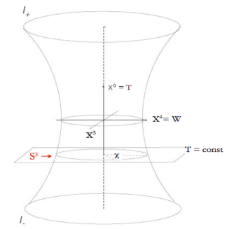
Figure 2: The de Sitter manifold represented as a single sheeted hyperboloid of revolution about the $T$ axis, in which the $X^{1}$, $X^{2}$ coordinates are suppressed. The hypersurfaces at constant $T$ are three-spheres, $\mathbb{S}^{3}$. The three-spheres at $T=\pm\infty$ are denoted by $I_{\pm}$.

The curvature tensor of de Sitter space satisfies

$$R^{ab}_{\ \ cd} = H^{2}\left(\delta^{a}_{\ c}\,\delta^{b}_{\ d}-\delta^{a}_{\ d}\,\delta^{b}_{\ c}\right)\,,$$ (68a)

$$R^{a}_{\ b} = 3H^{2}\,\delta^{a}_{\ b}\,,$$ (68b)

$$R = 12H^{2}\,,$$ (68c)

The Lie algebra $so(4,1)$ is generated by the generators of the Lorentz group in the $4+1$ dimensional flat embedding spacetime (66). In the coordinate (adjoint) representation the $10$ anti-Hermitian generators of this symmetry are

$$L_{\scriptscriptstyle AB}=X_{\scriptscriptstyle A}\frac{\partial}{\partial X^{\scriptscriptstyle B}}-X_{\scriptscriptstyle B}\frac{\partial}{\partial X^{\scriptscriptstyle A}}=-L_{\scriptscriptstyle BA}$$ (69)

These $10$ generators satisfy

$$[L_{\scriptscriptstyle AB},L_{\scriptscriptstyle CD}]=-\eta_{\scriptscriptstyle AC}\,L_{\scriptscriptstyle BD}+\eta_{\scriptscriptstyle BC}\,L_{\scriptscriptstyle AD}-\eta_{\scriptscriptstyle BD}\,L_{\scriptscriptstyle AC}+\eta_{\scriptscriptstyle AD}\,L_{\scriptscriptstyle BC}\,,$$ (70)

the Lie algebra $so(4,1)$. De Sitter space has $10$ Killing vectors corresponding to these $10$ generators.

The hyperbolic coordinates of de Sitter space are defined by

$$T = \frac{1}{H}\,\sinh u\,,$$ (71a)

$$W = \frac{1}{H}\,\cosh u\,\cos\chi\,,$$ (71b)

$$X^{i} = \frac{1}{H}\,\cosh u\,\sin\chi\,\hat{n}^{i}\,,\qquad i=1,2,3\,.$$ (71c)

where

$$\hat{n}=(\sin\theta\,\cos\phi\,,\sin\theta\,\sin\phi\,,\cos\theta)$$ (72)

is the unit vector on $\mathbb{S}^{2}$, and cast the de Sitter line element in the form

$$ds^{2}=\frac{1}{H^{2}}\left[-du^{2}+\cosh^{2}u\,(d\chi^{2}+\sin^{2}\chi\,d\Omega^{2})\right]\,.$$ (73)

The quantity in round parentheses is

$$d\Omega_{3}^{2}\equiv[d(\sin\chi\,\hat{n}^{i})]^{2}+[d(\cos\chi)]^{2}=d\chi^{2}+\sin^{2}\chi\,d\Omega^{2}\,,$$ (74)

the standard round metric on $\mathbb{S}^{3}$. Hence in the geodesically complete coordinates of (71) the de Sitter line element (73) is an hyperboloid of revolution whose constant $u$ sections are three spheres, represented in Fig. 2, which are invariant under the $O(4)$ subgroup of $O(4,1)$. It is sometimes convenient to define the hyperbolic conformal time coordinate $\upsilon$ by $\sec\upsilon=\cosh u$, so that (73) becomes

$$ds^{2}=H^{-2}\sec^{2}\upsilon\left(-d\upsilon^{2}+d\Omega_{3}^{2}\right)\,,$$ (75)

conformal to the Einstein static cylinder with $-\pi/2\leq\upsilon\leq\pi/2$.

In cosmology it is more common to use instead the Friedmann-Lemaître-Robertson-Walker (FLRW) line element with flat $\mathbb{R}^{3}$ spatial sections, viz.

$$ds^{2} = -d\tau^{2}+a^{2}(\tau)\,d\vec{x}\cdot d\vec{x}=-d\tau^{2}+a^{2}(\tau)\,(dx^{2}+dy^{2}+dz^{2})$$ (76)

$$= -d\tau^{2}+a^{2}(\tau)(d\varrho^{2}+\varrho^{2}d\Omega^{2})\,.$$

De Sitter space can be brought in the FLRW form by setting

$$T = \frac{1}{2H}\left(a-\frac{1}{a}\right)+\frac{Ha}{2}\,\varrho^{2}\,,$$ (77a)

$$W = \frac{1}{2H}\left(a+\frac{1}{a}\right)-\frac{Ha}{2}\,\varrho^{2}\,,$$ (77b)

$$X^{i} = a\,\varrho\,\hat{n}^{i}\,,$$ (77c)

with

$$a(\tau) = e^{H\tau}$$ (78a)

$$\varrho = |\vec{x}|=\sqrt{x^{2}+y^{2}+z^{2}}\,.$$ (78b)

From (77) and (78), $T+W\geq 0$ in these coordinates. Hence the flat FLRW coordinates cover only one half of the full de Sitter hyperboloid, with the hypersurfaces of constant RW time $\tau$ slicing the hyperboloid in Fig. 2 at a $45^{\circ}$ angle.

The change of time variable to the conformal time coordinate,

$$\eta=-H^{-1}e^{-H\tau}=-\frac{1}{Ha}\,,\qquad a=-\frac{1}{H\eta}\,,$$ (79)

is also often used to express the de Sitter line element is the conformally flat form

$$ds^{2}=a^{2}\,(-d\eta^{2}+d\vec{x}^{2})=\frac{1}{H^{2}\eta^{2}}\,(-d\eta^{2}+d\vec{x}^{2})\,.$$ (80)

¿From (71) and (77),

$$\cosh u\,\sin\chi=H\varrho\,a = -\frac{\varrho}{\eta}\,,$$ (81a)

$$\sinh u+\cosh u\,\cos\chi=a = -\frac{1}{H\eta}\,,$$ (81b)

which gives the direct relation between hyperbolic coordinates and flat FLRW coordinates.

The de Sitter static coordinates $(t,r,\theta,\phi)$ are defined by

$$T = \frac{1}{H}\,\sqrt{1-H^{2}r^{2}}\,\sinh(Ht)\,,$$ (82a)

$$W = \frac{1}{H}\,\sqrt{1-H^{2}r^{2}}\,\cosh(Ht)\,$$ (82b)

$$X^{i} = r\,\hat{n}^{i}\,.$$ (82c)

They bring the line element (66) into the static, spherically symmetric form (1) with (64), i.e.

$$ds^{2}=-(1-H^{2}r^{2})\,dt^{2}+\frac{dr^{2}}{(1-H^{2}r^{2})}+r^{2}d\Omega^{2}\,.$$ (83)

Just as in the Schwarzschild case (2) these static coordinates cover only part of the analytically fully extended de Sitter manifold (67). From (82), real static $(t,r)$ coordinates cover only the quarter of the de Sitter manifold where $W\geq 0$ and both $W\pm T\geq 0$. This quarter is represented as the rightmost wedge of the Carter-Penrose conformal diagram of de Sitter space in Fig. 3.

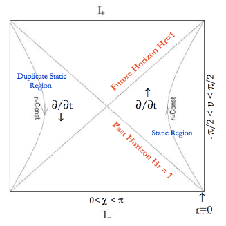
Figure 3: The Carter-Penrose conformal diagram for de Sitter space. Future and past infinity are at $I_{\pm}$. Only the quarter of the diagram labeled as the static region are covered by the static coordinates of (83). The orbits of the static time Killing field $\partial/\partial t$ are shown. The angular coordinates $\theta,\phi$ are again suppressed.

The Regge-Wheeler radial coordinate $r^{*}$ can be defined in the static frame by

$$r^{*} = \frac{1}{2H}\,\ln\left(\frac{1+Hr}{1-Hr}\right)=\frac{1}{H}\,\tanh^{-1}(Hr)\,,$$ (84a)

$$r = \frac{1}{H}\,\tanh(Hr^{*})\,\qquad{\rm so\ that}$$ (84b)

$$dr^{*} = \frac{dr}{1-H^{2}r^{2}}\,,\qquad\sqrt{1-H^{2}r^{2}}={\rm sech}(Hr^{*})\,,$$ (84c)

and

$$ds^{2} = {\rm sech}^{2}(Hr^{*})\,(-dt^{2}+dr^{*\,2})+\frac{1}{H^{2}}\tanh^{2}(Hr^{*})\,d\Omega^{2}$$ (85)

$$= \frac{1}{H^{2}}\,{\rm sech}^{2}(Hr^{*})\,\left[-H^{2}dt^{2}+H^{2}dr^{*\,2}+\sinh^{2}(Hr^{*})\,d\Omega^{2}\right].\qquad$$

Note that the horizon at $r=H^{-1}=r_{{}_{H}}$ is mapped to $r^{*}=\infty$ in these coordinates, and that the spatial part of the line element (85) in square brackets (the “optical” metric) is

$$ds^{2}_{opt}=H^{2}dr^{*\,2}+\sinh^{2}(Hr^{*})\,d\Omega^{2}=4\,\frac{d\vec{\sf y}\cdot d\vec{\sf y}}{(1-{\sf y}^{2})^{2}}$$ (86)

where the second form is obtained by defining

$$\vec{\sf y} \equiv {\sf y}\,\hat{n}\,,$$ (87a)

$${\sf y} \equiv \tanh\left(\frac{Hr^{*}}{2}\right)=\frac{Hr}{1+\sqrt{1-H^{2}r^{2}}}\quad{\rm so\ that}$$ (87b)

$$r = \frac{2}{H}\frac{\sf y}{1+{\sf y}^{2}}\,,\qquad r^{*}=\frac{1}{H}\,\ln\left(\frac{1+{\sf y}}{1-{\sf y}}\right)\,.$$ (87c)

Eq. (86) is a standard form of the line element of three-dimensional Łobachewsky (hyperbolic or Euclidean anti-deSitter) space ${\mathbb{H}}^{3}$. Thus, one expects conformal field theory (CFT) behavior at the horizon boundary, ${\sf y}=1$, $r=r_{{}_{H}}$ . This is reflected also in the wave eq. analogous to (30) in which the corresponding potential $V_{\ell}$ of (100) vanishes at the horizon, which we consider in the next subsection.

Since these various coordinatizations of the de Sitter manifold are quite different globally, and involve singular coordinate transformations at the horizon, much of the discussion of the Schwarzschild geometry have their analogs in de Sitter spacetime. The Carter-Penrose conformal diagram for the analytically extended de Sitter hyperboloid, Fig. 3 is similar to the corresponding diagram in the Schwarzschild case, Fig. 1. In each case the horizon is bifurcate (i.e. has two distinct parts) and the region covered by the static coordinates (83) is duplicated by a second region centered on the antipodal point of $\mathbb{S}^{3}$ where the sense of increasing static time $t$ is reversed. Thus the static Killing vector $K^{a}$ (47) becomes null on either horizon and spacelike in the upper and lower quarter wedges of Fig. 3.

III.3 Quantum Effects in de Sitter Spacetime

Quantum fluctuations and their backreaction effects in de Sitter spacetime were considered in EMfluc ; EMdSp ; EMSt ; EMdSMM ; EMtime . These studies indicate that fluctuations at the horizon scale $r_{{}_{H}}$ are responsible for important backreaction effects on the classical de Sitter expansion that could potentially relax the effective cosmological vacuum energy to zero. The authors of Refs. Wood have performed a perturbative analysis of long wavelength gravitational fluctuations in non de Sitter invariant initial states up to two-loop order. This work indicates the presence of secular terms in the quantum stress tensor of fluctuations about de Sitter space, tending to decrease the effective vacuum energy density, consistent with the earlier considerations in Refs. EMfluc ; EMdSp ; EMSt ; EMdSMM ; EMtime . The authors of Ref. MAB have studied the stress tensor for long wavelength cosmological perturbations in inflationary models as well, and also found a backreaction effect of the right sign to slow inflation. See also Refs. AW , IWald , and a discussion of these various approaches in Ref. NJP .

One of the first indications of non-trivial quantum effects in de Sitter spacetime is particle creation EMdSp . A space or time dependent background field generally creates particles. Schwinger first studied this effect in QED in a series of classic papers Schwinger . The rate of spontaneous decay of the electric field into charged particles is

$$\Gamma=\frac{(eE)^{2}}{c\hbar^{2}\pi^{2}}\exp\left(-\frac{m^{2}c^{3}}{eE\hbar}\right)$$ (88)

in the limit $eE\ll m^{2}c^{3}/\hbar$. From this point of view the exponential de Sitter expansion (76)-(78) provides a time dependent background field which can create particle pairs from the “vacuum,” converting the energy of the classical gravitational background into that of particle modes. The rate of this spontaneous creation of matter in de Sitter space can be calculated in analogy to the Schwinger effect in an electric field, with a similar result for the decay rate per unit volume EMdSp ,

$$\Gamma=\frac{16H^{4}}{\pi^{2}}\exp\left(-\frac{2\pi m}{\hbar H}\right)$$ (89)

for a scalar massive field with arbitrary curvature coupling (i.e. $m^{2}=\mu^{2}+\xi R=\mu^{2}+12\xi H^{2}$).

In the case of a spatially uniform electric field (and no magnetic fields) the Maxwell equation,

$$\frac{\partial\vec{E}}{\partial t}=-\langle\vec{j}\rangle$$ (90)

indicates that the creation of these particle pairs tends (at least initially) to decrease the strength of the electric field. In cosmology the Friedmann equation,

$$\left(\frac{\dot{a}}{a}\right)^{2}=H^{2}=\frac{8\pi G}{3}\,\rho\,,$$ (91)

together with the equation of covariant energy conservation,

$${\dot{\rho}}+3\,H\,(\rho+p)=0,$$ (92)

(with over dots here denoting differentiation with respect to proper time $\tau$) imply that

$${\dot{H}}=-\frac{4\pi G}{c^{2}}\ (\rho+p).$$ (93)

In both cases there is a classical static background that solves the equation trivially, namely $H$ or $\vec{E}$ a constant with zero source terms on the right hand side of (90) or (93). In the case of (93) this is de Sitter spacetime with $\rho_{\Lambda}+p_{\Lambda}=0$. Any creation of matter with $\rho+p>0$ will tend to decrease the strength of the classical background field $H$. The particle creation process has been studied in greater detail in the electric field KlugMot and de Sitter HabMolMot cases, and backreaction effects were also taken into account in the QED case the large $N$ limit KlugMot . In this limit self-interactions between the created charge particles are neglected, but such scatterings are essential to the final decay of the coherent classical field into particles. In the gravitational case it has so far not been feasible to carry out a full dynamical calculation of backreaction and particle scattering which would establish $\rho+p>0$ and final decay of the background value of $H$. Unlike electromagnetism in gravity there are massless particles which couple to the background field, and from (89) these will give the largest effect. However for minimally coupled massless scalar particles and for gravitons themselves, the definition of the “vacuum” state becomes more subtle, so that computing the infrared effects of massless particles and their interactions requires a different approach.

One possible way to define a preferred state of a system is by its symmetries. Since the symmetry group of the maximally analytically extended de Sitter hyperboloid is $O(4,1)$, a maximally $O(4,1)$ symmetric state can be defined, for most field theories, including massive and massless conformally invariant fields, such as the photon. Since under analytic continuation of $T\rightarrow iT$ the de Sitter manifold becomes $\mathbb{S}^{4}$, which is compact, one can define a state by the requirement of maximal $O(5)$ invariance, regularity on $\mathbb{S}^{4}$, whose $n$-point functions are all analytic under the continuation. This is often referred to as the Bunch-Davies (BD) state in the literature BD . Since the Euclidean $\mathbb{S}^{4}$ radius is $r_{{}_{H}}$, the Euclidean Green’s functions are periodic in imaginary time with period $2\pi r_{{}_{H}}/c$. This is again the KMS property of a thermal Green’s function, and hence the BD state defined by this analytic continuation from $\mathbb{S}^{4}$ is a thermal state with temperature GibPer ; GibEin79 ,

$$T_{{}_{H}}=\frac{\hbar H}{2\pi k_{{}_{B}}}\,,$$ (94)

the Hawking temperature of de Sitter space. Hence the BD state in de Sitter space is not a “vacuum” state, but is a state thermally populated with quanta at temperature $T_{{}_{H}}$. In this respect it is rather like the Hartle-Hawking state in the Schwarzschild background. In these fully time symmetric states there is no net particle creation on average and no decay rate. Because of the full $O(4,1)$ symmetry of the BD state, the expectation value of the energy-momentum tensor of any matter fields in this state must itself be of the form of a quantum correction to the cosmological term with $\rho=-p\sim H^{4}$ constant. The BD state usually assumed, tacitly or explicitly in models of inflation. It is interesting that because of infrared divergences the BD state does not exist for massless, minimally coupled scalar fields and gravitons themselves AllFol , which implies that these fields must be in a state with less than the full $O(4,1)$ de Sitter symmetry. Once the de Sitter symmetry is broken, however, it is not clear what the residual symmetry and final state of the system is, or how to go about determining it.

Even the existence of a maximally symmetric state does not guarantee its stability against small fluctuations. For example, it can be shown that in the uniform constant electric field background there are exactly $10$ isometries, the same number as with zero external field Beers . Thus one can construct mathematically a state which respects all these isometries, including a discrete symmetry corresponding to time reversal invariance, and no net pair creation, without necessarily guaranteeing the stability of the vacuum against pair creation in an external electric field. A subtle point, easily overlooked in Schwinger’s elegant effective action method, is that either time asymmetric boundary/initial conditions must be specified in such a decay problem, or it must be shown that the time symmetric state is dynamically unstable to quantum fluctuations, spontaneously breaking the larger isometry group to a smaller subgroup.

One may construct an argument analogous to that in the Schwarzschild case that the de Sitter invariant BD should be quantum mechanically unstable, under fluctuations in its Hawking temperature. Note that the vacuum energy within a spherical volume of radius $r_{{}_{H}}$ is

$$E_{{}_{H}}=\frac{4\pi r_{{}_{H}}^{3}}{3}\,\rho_{\Lambda}=\frac{c^{4}}{2G}\ \frac{1}{H}\,,$$ (95)

which is inversely proportional to (94). Therefore,

$$\frac{dE_{{}_{H}}}{dT_{{}_{H}}}=-\frac{E_{{}_{H}}}{T_{{}_{H}}}=-\frac{\pi c^{3}k_{{}_{B}}}{GH^{2}}<0\,,$$ (96)

and the heat capacity of the region of de Sitter space within one horizon volume is apparently negative. This indicates that if the region can exchange energy with its environment external to the cosmological horizon, the BD thermal state will be unstable to such energy exchanges, analogously to the black hole case. The problem of negative heat capacity is also similar.

It has also been suggested that the Bekenstein-Hawking $1/4$ area formula for the entropy

$$S_{{}_{H}}\stackrel{{\scriptstyle?}}{{=}}k_{{}_{B}}\frac{A_{H}}{4L_{pl}^{2}}=\frac{\pi c^{5}k_{{}_{B}}}{\hbar GH^{2}}$$ (97)

be taken over to the de Sitter case GibHaw . However what degrees of freedom this “entropy” counts are even less clear than in the black hole case. Note also that from (95)

$$dE_{{}_{H}} = d(\rho_{\Lambda}V_{{}_{H}})=d\rho_{\Lambda}\,V_{{}_{H}}+\rho_{\Lambda}\,dV_{{}_{H}}$$ (98)

$$= d\rho_{\Lambda}V_{{}_{H}}-p_{\Lambda}dV_{{}_{H}}$$

$$\neq T_{{}_{H}}dS_{{}_{H}}-p_{\Lambda}dV_{{}_{H}}\,.$$

In fact $T_{{}_{H}}dS_{{}_{H}}$ and $d\rho_{\Lambda}V_{{}_{H}}$ have opposite signs. This implies that $S_{{}_{H}}$ cannot be interpreted as an entropy and/or additional contributions, such as surface terms, are missing from (98).

Like the Schwarzschild case, de Sitter spacetime admits a static Killing field which is timelike in one region of its maximal analytic extension. If one considers any thermal state with a temperature $T$ different from $T_{{}_{H}}$, defined with respect to the static Killing time in one patch of de Sitter space, then the renormalized stress-energy tensor is AndHis

$$\langle T^{a}_{\ b}\rangle_{{}_{R}}\rightarrow\frac{\pi^{2}}{90}\,\frac{k_{{}_{B}}^{4}}{(\hbar c)^{3}}\,(T^{4}-T_{{}_{H}}^{4})\left(1-H^{2}r^{2}\right)^{-2}\,{\rm diag}\,(-3,1,1,1)\,,$$ (99)

as $r\rightarrow r_{{}_{H}}$, analogous to (45) in the Schwarzschild case. Thus any finite deviation of the temperature from the Hawking-de Sitter temperature (94) in the region interior to the horizon will produce a arbitrarily large stress-energy on the horizon. The previous discussion in Sec. II about the dependence of $\langle T^{a}_{\ b}\rangle_{{}_{R}}$ on the gauge invariant but non-local norm of the static Killing vector field, the non-commutivity of the limits $\hbar\rightarrow 0$ and $r\rightarrow r_{{}_{H}}$, and the breakdown of the analytic continuation hypothesis through coordinate or conical singularities apply to the de Sitter case as well.

The wave equation of a quantum field propagating in de Sitter space can also be separated in the static coordinates (83). By following the analogous steps as used in (28)-(32) in the Schwarzschild case, one arrives at the identical form of the radial scattering eq. (30) in terms of the $r^{*}$ coordinate (84), with the scattering potential in de Sitter space given by

$$V_{\ell}\big{|}_{dS}=(1-H^{2}r^{2})\left[\frac{\ell(\ell+1)}{r^{2}}+\mu^{2}+2H^{2}(6\xi-1)\right]$$

$$=H^{2}\left[\ell(\ell+1)\,{\rm csch}^{2}(Hr^{*})+\left(\frac{1}{4}-\nu^{2}\right){\rm sech}^{2}(Hr^{*})\right],$$ (100)

where $-\xi/2$ is the $R\Phi^{2}$ coupling in the scalar field Lagrangian, and

$$\nu\equiv\sqrt{\frac{9}{4}-\frac{\mu^{2}}{H^{2}}-12\xi}\,.$$ (101)

A significant difference of the effective one dimensional scattering problem of spherical waves in the de Sitter case is that the coordinate singularity at the origin $r=0$ is in the physical range, compared to the Schwarzschild case in which the $r^{*}$ coordinate range $(-\infty,\infty)$ covers only the exterior Schwarzschild geometry. Thus in order to avoid a singularity at the origin we must require that the scattering solutions to (30) with (100) satisfy

$$f_{\omega\ell}\big{|}_{dS}\sim r^{\ell(\ell+1)}\qquad{\rm as}\qquad r\rightarrow 0\,,$$ (102)

thereby excluding a possible singular $r^{-\ell}$ behavior for $\ell\geq 1$. This means that in de Sitter space only the particular linear combination of ingoing and outgoing solutions of the corresponding (30) vanishing at the origin should be used in the quantization of the $\Phi$ field and not the general linear combination in (33)-(35) appropriate in the Schwarzschild background. As a corollary this implies that there can be no analog of the Unruh state in de Sitter spacetime, since (102) is equivalent to the requirement of no net flux into or out of the origin at $r=0$ in static de Sitter coordinates (83). Otherwise the quantization of a scalar field in de Sitter space in these coordinates is analogous to the Schwarzschild case, and one can again easily find states regular at the origin which have diverging stress tensors on the horizon, as in (99). The appearance of such states and large stress tensors would necessarily mean large quantum backreaction effects in the vicinity of the horizon $r=r_{{}_{H}}$, and the breakdown of $O(4,1)$ de Sitter symmetry down to $O(3)$, with perhaps a very different global geometry than the analytic continuation implied by extending the coordinates (73) globally. As in the Schwarzschild case, this is ultimately a question of physics, not simply mathematical analytic continuation of coordinates.

The earlier work on the behavior of the graviton propagator in de Sitter space AMJMP ; AlTur ; FIT also indicates the existence of infrared divergent contributions to correlations at large distances. This violates cluster decomposition and makes the definition of a graviton scattering matrix in global de Sitter space problematic. The existence of long distance correlations and infrared divergences is a signal of the breakdown of the global BD state. The relevance of matter self-interactions, first studied in Refs. Mhyr ; Ford has been taken up again recently in Refs. Poly0810 , where the phenomenon of runaway stimulated emission in de Sitter space is explored. This adds to the by now substantial literature on non-trivial quantum infrared behavior in de Sitter space NJP . Since infrared effects are the common feature of all these studies, one might well suppose that there should be some relevant operator(s) in the low energy effective theory of gravity which describes in a general and universal way (i.e. independently of specific matter self-interactions) the quantum effects of matter/radiation fields on the macroscopic scales of both the black hole and cosmological horizons, and which points to a possible resolution of the physics in both cases. This is what a predictive effective field theory (EFT) approach should provide.

IV Effective Field Theory: The Role of Anomalies

The important role of quantum anomalies in the low energy effective field theory approach to the strong interactions is reviewed in this section, and their relevance to the EFT of gravity discussed. The first and best known example of this is the axial anomaly in QED and QCD. Since the two-particle correlations that give rise to non-trivial infrared effects can be seen already in this flat space case, we digress and review that here before returning to the curved spacetime application in gravity.

IV.1 The Axial Anomaly in QED and QCD

Although the triangle axial anomaly in both QED has been known for some time Adler ; BellJack ; Jackcurr , the general behavior of the amplitude off mass shell, its spectral representation, the appearance of a massless pseudoscalar pole in the limit of zero fermion mass, and the infrared aspects of the anomaly generally have received only limited attention DolZak ; Horej . It is this generally less emphasized infrared character of the axial anomaly which will be important for our EFT considerations in gravity, so we begin by reviewing this aspect of the axial anomaly in QED in some detail.

The vector and axial currents in QED are defined by

$$J^{\mu}(x)=\bar{\psi}(x)\gamma^{\mu}\psi(x)\,.$$ (103a)

$$J_{5}^{\mu}(x)=\bar{\psi}(x)\gamma^{\mu}\gamma^{5}\psi(x)\,.$$ (103b)

The Dirac eq.,

$$-i\gamma^{\mu}(\partial_{\mu}-ieA_{\mu})\psi+m\psi=0\,.$$ (104)

implies that the vector current is conserved,

$$\partial_{\mu}J^{\mu}=0\,,$$ (105)

while the axial current apparently obeys

$$\partial_{\mu}J_{5}^{\mu}=2im\,\bar{\psi}\gamma^{5}\psi\qquad{\rm(classically)}.$$ (106)

In the limit of vanishing fermion mass $m\rightarrow 0$, the classical Lagrangian has a $U_{ch}(1)$ global symmetry under $\psi\rightarrow e^{i\alpha\gamma^{5}}\psi$, in addition to $U(1)$ local gauge invariance, and $J_{5}^{\mu}$ is the Noether current corresponding to this chiral symmetry. As is well known, both symmetries cannot be maintained simultaneously at the quantum level. Let us denote by $\langle J_{5}^{\mu}(z)\rangle_{{}_{A}}$ the expectation value of the chiral current in the presence of a background electromagnetic potential $A_{\mu}$. Enforcing $U(1)$ gauge invariance (105) on the full quantum theory leads necessarily to a finite axial current anomaly,

$$\partial_{\mu}\langle J_{5}^{\mu}\rangle_{{}_{A}}\Big{|}_{m=0}=\frac{e^{2}}{16\pi^{2}}\ \epsilon^{\mu\nu\rho\sigma}F_{\mu\nu}F_{\rho\sigma}=\frac{e^{2}}{2\pi^{2}}\,\vec{E}\cdot\vec{B}\,,$$ (107)

in an external electromagnetic field. Varying this expression twice with respect to the external $A$ field we see that anomaly must appear in the amplitude,

$$\Gamma^{\mu\alpha\beta}(p,q)\equiv-i\int d^{4}x\int d^{4}y\,e^{ip\cdot x+iq\cdot y}\ \frac{\delta^{2}\langle J_{5}^{\mu}(0)\rangle_{{}_{A}}}{\delta A_{\alpha}(x)\delta A_{\beta}(y)}\Bigg{|}_{A=0}$$

$$=ie^{2}\int d^{4}x\int d^{4}y\,e^{ip\cdot x+iq\cdot y}\ \langle{\cal T}J_{5}^{\mu}(0)J^{\alpha}(x)J^{\beta}(y)\rangle\big{|}_{A=0}\,.$$ (108)

At the lowest one-loop order it is given by the triangle diagram of Fig. 4, plus the Bose symmetrized diagram with the photon legs interchanged.

Figure 4: The triangle diagram contributing to the axial current anomaly. The four-momentum of integration is $l$.

Elementary power counting indicates that the triangle diagram of Fig. 4 is superficially linearly divergent. The formal reason why (105) and (106) cannot both be maintained at the quantum level is that verifying them requires the ability to shift the loop momentum integration variable $l$ in the triangle amplitude. Because the diagram is linearly divergent, such shifts are inherently ambiguous, and can generate finite extra terms. It turns out that there is no choice for removing the ambiguity which satisfies both the vector and chiral Ward identities simultaneously, and one is forced to choose between them. Thus although the ambiguity results in a well-defined finite term, the axial anomaly has most often been presented as inherently a problem of regularization of an apparently ultraviolet linearly divergent loop integral Adler ; BellJack ; Jackcurr .

There is an alternative derivation of the axial anomaly that emphasizes instead its infrared character. The idea of this approach is to use the tensor structure of the triangle amplitude to extract its well-defined ultraviolet finite parts, which are homogeneous of degree three in the external momenta $p$ and $q$. Then the remaining parts of the full amplitude may be determined by the joint requirements of Lorentz covariance, Bose symmetry under interchange of the two photon legs, and electromagnetic current conservation,

$$p_{\alpha}\Gamma^{\mu\alpha\beta}(p,q)=0=q_{\beta}\Gamma^{\mu\alpha\beta}(p,q)\,,$$ (109)

at the two vector vertices. By this method the full one-loop triangle contribution to $\Gamma^{\mu\alpha\beta}(p,q)$, becomes completely determined in terms of well-defined ultraviolet finite integrals which require no further regularization Rosenb ; Horejb . The divergence of the axial current may then be computed unambiguously, and one obtains (107) in the limit of vanishing fermion mass. It is this latter method which makes clear that the anomaly is a consequence of symmetries of the low energy theory, no matter how its UV behavior is tamed, provided only that the regularization respects these symmetries. There is of course no contradiction between these two points of view, since it is the same Ward identities which are imposed in either method, and in any case in the conformal limit of vanishing fermion mass the infrared and ultraviolet behavior of the triangle amplitude are one and the same.

The details of the calculation by this method may be found in Refs. Rosenb ; Horejb ; GiaMot . One first uses the Poincaré invariance of the vacuum to assert that $\Gamma^{\mu\alpha\beta}(p,q)$ can be expanded in the set of all three-index tensors constructible from the $p$ and $q$, with the correct Lorentz transformation properties. There are exactly eight such tensors, two of which are linear in $p$ or $q$, namely $\varepsilon^{\mu\alpha\beta\lambda}p_{\lambda}$ and $\varepsilon^{\mu\alpha\beta\lambda}q_{\lambda}$, while the remaining six are homogeneous of degree three in the external momenta. However only certain linear combinations of these eight tensors satisfy (109). Define first the two index tensor,

$$\upsilon^{\alpha\beta}(p,q)\equiv\epsilon^{\alpha\beta\rho\sigma}p_{\rho}q_{\sigma}\,,$$ (110)

which satisfies

$$\upsilon^{\alpha\beta}(p,q) = \upsilon^{\beta\alpha}(q,p)\,,$$ (111a)

$$p_{\alpha}\upsilon^{\alpha\beta}(p,q)= 0 =q_{\beta}\upsilon^{\alpha\beta}(p,q)\,.$$ (111b)

Then the six third rank tensors, $\tau_{i}^{\mu\alpha\beta}(p,q)$, $i=1,\dots,6$ which satisfy the conditions (109),

$$p_{\alpha}\tau_{i}^{\mu\alpha\beta}(p,q)=0=\tau_{i}^{\mu\alpha\beta}(p,q)\,q_{\beta}=0\,,\qquad i=1,\dots,6,$$ (112)

are given in Table 1.

$$\begin{array}[]{|@{\hspace{.8cm}}c @{\hspace{.8cm}}|@{\hspace{.8cm}}c @{\hspace{.8cm}}|}\hline\cr\hskip 22.76228pt\lx@intercol\hfil i\hfil\hskip 22.76228pt\vrule\hskip 22.76228pt&\tau_{i}^{\mu\alpha\beta}(p,q)\hfil\hskip 22.76228pt\\ \hline\cr\hline\cr\hskip 22.76228pt\lx@intercol\hfil 1\hfil\hskip 22.76228pt\vrule\hskip 22.76228pt&-p\cdot q\,\epsilon^{\mu\alpha\beta\lambda}p_{\lambda}-p^{\beta}\,\upsilon^{\mu\alpha}(p,q)\hfil\hskip 22.76228pt\\ \hline\cr\hskip 22.76228pt\lx@intercol\hfil 2\hfil\hskip 22.76228pt\vrule\hskip 22.76228pt&p^{2}\epsilon^{\mu\alpha\beta\lambda}q_{\lambda}\,+p^{\alpha}\upsilon^{\mu\beta}(p,q)\hfil\hskip 22.76228pt\\ \hline\cr\hskip 22.76228pt\lx@intercol\hfil 3\hfil\hskip 22.76228pt\vrule\hskip 22.76228pt&p^{\mu}\,\upsilon^{\alpha\beta}(p,q)\hfil\hskip 22.76228pt\\ \hline\cr\hline\cr\hskip 22.76228pt\lx@intercol\hfil 4\hfil\hskip 22.76228pt\vrule\hskip 22.76228pt&p\cdot q\,\epsilon^{\mu\alpha\beta\lambda}q_{\lambda}+q^{\alpha}\,\upsilon^{\mu\beta}(p,q)\hfil\hskip 22.76228pt\\ \hline\cr\hskip 22.76228pt\lx@intercol\hfil 5\hfil\hskip 22.76228pt\vrule\hskip 22.76228pt&-q^{2}\varepsilon^{\mu\alpha\beta\lambda}p_{\lambda}\,-q^{\beta}\upsilon^{\mu\alpha}(p,q)\hfil\hskip 22.76228pt\\ \hline\cr\hskip 22.76228pt\lx@intercol\hfil 6\hfil\hskip 22.76228pt\vrule\hskip 22.76228pt&q^{\mu}\,\upsilon^{\alpha\beta}(p,q)\hfil\hskip 22.76228pt\\ \hline\cr\end{array}$$

Table 1: The $6$ third rank (pseudo)tensors obeying (112)

Hence we may express the amplitude (108) satisfying (109) as a linear combination,

$$\Gamma^{\mu\alpha\beta}(p,q)=\sum_{i=1}^{6}f_{i}\,\tau_{i}^{\mu\alpha\beta}(p,q)\,,$$ (113)

where $f_{i}=f_{i}(k^{2};p^{2},q^{2})$ are dimension $-2$ scalar functions of the three invariants, $p^{2},q^{2}$, and $k^{2}$. Note from Table 1 that the two tensors of dimension one which could potentially have logarithmically divergent scalar coefficient functions occur only in linear combination with dimension three tensors. Hence the coefficient functions $f_{i}$ of these linear combinations obeying (109) are all ultraviolet finite. These finite contributions can be obtained unambiguously from the imaginary part of the triangle graph of Fig. 5, which are finite a priori and then determining the real part from the imaginary part by an unsubtracted, i.e. UV finite dispersion relation. This leads to the finite coefficients given in the literature Rosenb ; Horejb ; GiaMot , viz.

$$f_{1}=f_{4}=\frac{e^{2}}{\pi^{2}}\int_{0}^{1}dx\int_{0}^{1-x}dy\ \frac{xy}{D}\,$$ (114a)

$$f_{2}=\frac{e^{2}}{\pi^{2}}\int_{0}^{1}dx\int_{0}^{1-x}dy\ \frac{x(1-x)}{D}\,,$$ (114b)

$$f_{5}=\frac{e^{2}}{\pi^{2}}\int_{0}^{1}dx\int_{0}^{1-x}dy\ \frac{y(1-y)}{D}\,,$$ (114c)

$$f_{3}=f_{6}=0\,,$$ (114d)

where the denominator of the Feynman parameter integral is

$$D\equiv p^{2}x(1-x)+q^{2}y(1-y)+2p\cdot q\,xy+m^{2}=(p^{2}\,x+q^{2}\,y)(1-x-y)+xy\,k^{2}+m^{2}\,,$$ (115)

strictly positive for $m^{2}>0$, and spacelike momenta, $k^{2},p^{2},q^{2}>0$.

Thus, the full amplitude $\Gamma^{\mu\alpha\beta}(p,q)$ satisfying

1. Lorentz invariance of the vacuum ,

2. Bose symmetry under interchange of photon lines ,

3. vector current conservation (109) ,

4. unsubtracted dispersion relation of real and imaginary parts ,

with the finite imaginary parts determined by the cut triangle diagram of Fig. 5, is given by (113) and (114), without any need of regularization of ultraviolet divergent loop integrals at any step.

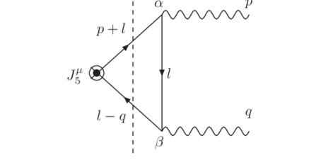
Figure 5: The discontinuous or imaginary part of the triangle diagram of Fig. 4 with respect to $k^{2}$. The propagators which are cut by the dashed line are replaced by their corresponding on-shell delta functions.

Since this amplitude is fully determined by (i)-(iv), its contraction with $k_{\mu}$, and the divergence of the axial vector current is determined as well. There is no further freedom to demand the naive axial Ward identity corresponding to (106). Instead we find

$$k_{\mu}\,\Gamma^{\mu\alpha\beta}(p,q)={\cal A}\,\upsilon^{\alpha\beta}(p,q)\,,$$ (116)

where

$${\cal A}(k^{2};p^{2},q^{2})=2p\cdot q\,f_{1}+p^{2}f_{2}+q^{2}f_{5}$$

$$=\frac{e^{2}}{\pi^{2}}\int_{0}^{1}dx\int_{0}^{1-x}dy\ \frac{D-m^{2}}{D}$$

$$\qquad=\frac{e^{2}}{2\pi^{2}}-\frac{e^{2}}{\pi^{2}}\ m^{2}\,\int_{0}^{1}dx\int_{0}^{1-x}dy\ \frac{1}{D}\,.$$ (117)

The second term proportional to $m^{2}$ is what would be expected from the naive axial vector divergence (106) Horejb . The first term in (117) in which the denominator $D$ is cancelled in the numerator is

$$\frac{e^{2}}{\pi^{2}}\int_{0}^{1}dx\int_{0}^{1-x}dy=\frac{e^{2}}{2\pi^{2}}\,,$$ (118)

and which remains finite and non-zero in the limit $m\rightarrow 0$ is the axial anomaly.

Thus the finite anomalous term is unambiguously determined by our four requirements above, and may be clearly identified even for finite $m$, when the chiral symmetry is broken. This construction of the amplitude from only symmetry principles and its finite parts may be regarded as a proof that the same finite axial anomaly must arise in any regularization of the original triangle amplitude which respects these symmetries and leaves the finite parts unchanged. Explicit calculations in dimensional regularization and Pauli-Villars regularization schemes, which respect these symmetries confirm this Bertl .

Now the important consequence of the anomaly in (117) in the divergence is that when the photons $p^{2}=q^{2}=0$ are on shell, the amplitude $\Gamma^{\mu\alpha\beta}(p,q)$ develops a simple pole at in $k^{2}$ as the electron mass $m\rightarrow 0$. This follows from the first line of (117) which shows that when $p^{2}=q^{2}=0$, $2p\cdot q=k^{2}$ so ${\cal A}$ is explicitly proportional to $k^{2}$. Since $\cal A$ is finite when $m\rightarrow 0$, the amplitude function $f_{1}(k^{2};0,0)$ must develop a pole in $k^{2}$. Indeed by explicit calculation from (114)-(115), we have

$$f_{1}(k^{2};p^{2}=0,q^{2}=0)\big{|}_{m=0}=\frac{e^{2}}{2\pi^{2}}\frac{1}{k^{2}}\,.$$ (119)

The corresponding imaginary part (discontinuity in $k^{2}$) becomes a $\delta(k^{2})$ in the same limit. Moreover, even for arbitrary $p^{2},q^{2},m^{2}\geq 0$, the spectral function obtained from this imaginary part obeys an ultraviolet finite sum rule Horejb ; GiaMot .

The appearance of a massless pseudoscalar pole (119) in the triangle anomaly amplitude in the massless fermion limit suggests that this can be described as the propagator of a pseudoscalar field which couples to the axial current. Indeed it is not difficult to find the field description of the pole. To do so let us note first that the axial current expectation value $\langle J_{5}^{\mu}\rangle_{{}_{A}}$ can be obtained from an extended action principle in which we introduce an axial vector field source, ${\cal B}_{\mu}$ into the Dirac Lagrangian,

$$i\bar{\psi}\gamma^{\mu}\left(\stackrel{{\scriptstyle\leftrightarrow}}{{\partial}}_{\mu}-ieA_{\mu}\right)\psi-m\bar{\psi}\rightarrow i\bar{\psi}\gamma^{\mu}\left(\stackrel{{\scriptstyle\leftrightarrow}}{{\partial}}_{\mu}-ieA_{\mu}-ig\gamma^{5}{\cal B}_{\mu}\right)\psi-m\bar{\psi}\psi$$ (120)

so that the variation of the corresponding action with respect to ${\cal B}_{\mu}$ gives

$$\frac{\delta{\cal S}}{\delta{\cal B}_{\mu}}=g\langle J_{5}^{\mu}\rangle_{{}_{A}}\,.$$ (121)

Henceforth we shall set the axial vector coupling $g=1$. Next let us decompose the axial vector ${\cal B}_{\mu}$ into its transverse and longitudinal parts,

$${\cal B}_{\mu}={\cal B}_{\mu}^{\perp}+\partial_{\mu}{\cal B}$$ (122)

with $\partial^{\mu}{\cal B}_{\mu}^{\perp}=0$ and $\cal B$ a pseudoscalar. Then, by an integration by parts in the action corresponding to (120), we have

$$\partial_{\mu}\langle J_{5}^{\mu}\rangle_{{}_{A}}=-\frac{\delta{\cal S}}{\delta{\cal B}}\,.$$ (123)

Thus the axial anomaly (107) implies that there is a term in the one-loop effective action in a background $A_{\mu}$ and ${\cal B}_{\mu}$ field, linear in $\cal B$ of the form,

$${\cal S}_{eff}=-\frac{e^{2}}{16\pi^{2}}\,\int d^{4}x\,\epsilon^{\mu\nu\rho\sigma}F_{\mu\nu}F_{\rho\sigma}\,{\cal B}\,,$$ (124)

or since $\partial^{\lambda}{\cal B}_{\lambda}=\,\raise 0.5pt\hbox{$\vbox{\hrule\hbox{\vrule height=6.50403pt\kern 6.50403pt\vrule} \hrule}$}\,{\cal B}$,

$${\cal S}_{eff}=-\frac{e^{2}}{16\pi^{2}}\,\int d^{4}x\int d^{4}y\ ,[\epsilon^{\mu\nu\rho\sigma}F_{\mu\nu}F_{\rho\sigma}]_{x}\,\raise 0.5pt\hbox{$\vbox{\hrule\hbox{\vrule height=6.50403pt\kern 6.50403pt\vrule} \hrule}$}\,^{-1}_{xy}\,[\partial^{\lambda}{\cal B}_{\lambda}]_{y}\,,$$ (125)

where $\,\raise 0.5pt\hbox{$\vbox{\hrule\hbox{\vrule height=6.50403pt\kern 6.50403pt\vrule} \hrule}$}\,^{-1}_{xy}$ is the Green’s function for the massless scalar wave operator $\,\raise 0.5pt\hbox{$\vbox{\hrule\hbox{\vrule height=6.50403pt\kern 6.50403pt\vrule} \hrule}$}\,=\partial_{\mu}\partial^{\mu}$. Thus from (121), this non-local action gives SmaiSpal

$$\langle J_{5}^{\mu}\rangle_{{}_{A}}=\frac{e^{2}}{16\pi^{2}}\partial^{\mu}\,\raise 0.5pt\hbox{$\vbox{\hrule\hbox{\vrule height=6.50403pt\kern 6.50403pt\vrule} \hrule}$}\,^{-1}\epsilon^{\alpha\beta\rho\sigma}F_{\alpha\beta}F_{\rho\sigma}\,,$$ (126)

which exhibts the massless scalar pole in the massless limit of (119), and which agrees with the explicit calculation of the physical $\langle 0|J_{5}^{\mu}|p,q\rangle$ triangle amplitude to two photons for $p^{2}=q^{2}=m^{2}=0$. The existence of this pole or $\delta$ function in the two-particle intermediate $e^{+}e^{-}$ intermediate state is the first indication that a phenomenon similar to Cooper pairing in condensed matter systems can exist in relativistic quantum field theory, and this effect is connected to anomalies.

In Ref. GiaMot a local action corresponding to (163) was found by introducing two pseudoscalar fields. The introduction of two fields is necessary if the only term in the effective action with this massless pole is the term (125) which is off-diagonal in $F\tilde{F}$ and $\partial\cdot{\cal B}$. If on the other hand the effective action contains the perfect square,

$$\int d^{4}x\left(\partial^{\lambda}{\cal B}_{\lambda}+\,\raise 0.5pt\hbox{$\vbox{\hrule\hbox{\vrule height=6.50403pt\kern 6.50403pt\vrule} \hrule}$}\,^{-1}F_{\mu\nu}\tilde{F}^{\mu\nu}\right)^{2}$$

then this effective action can be represented by a single pseudoscalar field. The possible existence of the additional terms in massless QED necessary to complete the square is currently under investigation,

Since it contains kinetic terms for the additional pseudoscalar field(s), the effective action of Ref. GiaMot describes additional pseudoscalar degree(s) of freedom. These degrees of freedom are two-particle $0^{-}$ correlated $e^{+}e^{-}$ states, composite bilinears of $\bar{\psi}$ and $\psi$, which appear in anomalous amplitudes as massless poles. In condensed matter physics, or electrodynamics at finite temperature or in polarizable media, where Lorentz invariance is broken, it is a familiar circumstance that there are low energy collective modes of the many body theory, which are not part of the single particle constituent spectrum. This occurs also in vacuo in the two dimensional massless Schwinger model, whose anomaly and longitudinal “photon” can be described by the introduction of an effective scalar field composed of an $e^{+}e^{-}$ pair LSB . In $3+1$ dimensions, relativistic kinematics and symmetries severely limit the possibilities for the appearance of such composite massless scalars, with the triangle anomaly the only known example ColGro . The fact that the $e^{+}e^{-}$ pair becomes collinear in the massless limit shows that this effectively reduces the dimensionality back to $1+1$. In the well studied $1+1$ dimensional case, the commutation relations of fermion bilinear currents $J^{\mu}$ and $J^{\nu}_{5}$, which create the composite $e^{+}e^{-}$ massless state are due to the anomaly AdBertHof . A similar phenomenon occurs in the triangle amplitude in $3+1$ dimensions. The axial anomaly thus implies additional long range correlations and collective degrees of freedom in the many body quantum theory, similar to Cooper pairs in a superconductor, which are not present in the classical or first quantized single particle theory.

In real QED these infrared effects are suppressed by the non-zero physical electron mass $m>0$, and the additional fact that macroscopic chirality violating sources for $J_{5}^{\mu}$ which would be sensitive to the anomaly are difficult to create. In QCD the situation is complicated both by the strong interactions in the infrared and the spontaneous breaking of chiral symmetry. The neutral member of the isotriplet of pseudoscalar Goldstone bosons in the low energy EFT is the $\pi^{0}$, whose decay to two photons, $\pi^{0}\rightarrow 2\gamma$ is correctly given by the triangle amplitude BarFriGM ; Wein . In fact, it was the experimental agreement between the measured decay rate to that predicted by the axial anomaly computed in the UV theory of $3$ colors of fractionally charged quarks that gave one of the strongest early confirmations of QCD. The fact that this amplitude is non-vanishing in the chiral limit, yet cannot be described by a local operator of dimension $4$ or less in the chiral Lagrangian, violates naive decoupling and illustrates how an anomaly couples UV to low energy physics. It is the fact that the anomaly may be computed in the UV theory of QCD but gives rise to a low energy amplitude of meson decay, $\pi^{0}\rightarrow 2\gamma$ that led to the principle of anomaly matching tHooft .

The apparent massless pseudoscalar anomaly pole of (119) in the isosinglet channel in the chiral limit of QCD is even more interesting. The $0^{-}$ state described by this pole in the isosinglet channel mixes with the pseudoscalar axial gluon density ${\cal Q}(x)=G^{a}_{\mu\nu}(x)\tilde{G}^{a\mu\nu}(x)$, and gives rise to a non-vanishing susceptibility of axial gluon densities,

$$\chi(k^{2})=\int d^{4}x\,e^{ik\cdot x}\langle{\cal Q}(x)\,{\cal Q}(0)\rangle\,,$$ (127)

as $k^{2}\rightarrow 0$, despite the fact that $\cal Q$ is a total derivative and therefore one would naively expect $\chi(k^{2})$ to be proportional to $k^{2}$ and vanish in this limit. The fact that the susceptibility $\chi(0)$ is non-vanishing is a direct effect of the massless anomaly pole Ven . The degree of freedom this infrared pole represents combines with a non-dynamical but gauge invariant ${\cal Q}^{2}$ term in the effective action of QCD to yield finally one propagating massive isosinglet psuedoscalar state which can be identified with the $\eta^{\prime}$ meson, solving the $U(1)$ problem in QCD Ven . Thus there is no doubt that the pseudoscalar $0^{-}$ state which appears in the isosinglet anomaly channel in perturbation theory is physical and propagating in the final S-matrix of the theory, but it becomes massive by a topological variant of the Higgs mechanism ATT .

The lesson to be taken away from this QCD example is that anomalies are a unique window which the low energy EFT provides to short distance physics. Two particle correlated pair states appear in anomalous amplitudes, which can be described as propagating massless fields that have consequences for low energy physics. The anomalous Ward identities and the long distance effects they generate must be taken into account by explicitly adding the IR relevant terms they induce in the low energy effective action BarFriGM ; Wein .

IV.2 The $\langle TJJ\rangle$ Triangle Amplitude in QED

In this section we consider the amplitude for the trace anomaly in flat space that most closely corresponds to the triangle amplitude for the axial current anomaly reviewed in the previous section, and give a complete calculation of the full $\langle T^{\mu\nu}J^{\alpha}J^{\beta}\rangle$ amplitude for all values of the mass and the off-shell kinematic invariants. Although the tensor structure of this amplitude is more involved than the axial vector case, the kinematics is essentially the same, and the appearance of the massless pole very much analogous to the axial case.

Classical fields satisfying wave equations with zero mass, which are invariant under conformal transformations of the spacetime metric, $g_{\mu\nu}\rightarrow e^{2\sigma}g_{ab}$ have stress tensors with zero classical trace, $T^{\mu}_{\ \mu}=0$. In quantum theory the stress tensor $T^{\mu}_{\ \nu}$ becomes an operator with fluctuations about its mean value. The mean value itself $\langle T^{\mu}_{\ \nu}\rangle$ is formally UV divergent, due to its zero point fluctuations, as in (59), and requires a careful renormalization procedure. The result of this renormalization consistent with covariant conservation in curved spacetime is that classical conformal invariance cannot be maintained at the quantum level. The trace of the stress tensor is generally non-zero when $\hbar\neq 0$, in non-trivial background fields, provided one preserves the covariant conservation of $T^{\mu}_{\ \nu}$ (a necessary requirement of any theory respecting general coordinate invariance and consistent with the Equivalence Principle) yields an expectation value of the quantum stress tensor with a non-zero trace.

The fundamental quantity of interest for us now is the expectation value of the energy-momentum tensor bilinear in the fermion fields in an external electromagnetic potential $A_{\mu}$,

$$\langle T^{\mu\nu}\rangle_{{}_{A}}=\langle T^{\mu\nu}_{free}\rangle_{{}_{A}}+\langle T^{\mu\nu}_{int}\rangle_{{}_{A}}\,$$ (128)

where

$$T^{\mu\nu}_{free}=-i\bar{\psi}\gamma^{(\mu}\!\!\stackrel{{\scriptstyle\leftrightarrow}}{{\partial}}\!^{\nu)}\psi+g^{\mu\nu}(i\bar{\psi}\gamma^{\lambda}\!\!\stackrel{{\scriptstyle\leftrightarrow}}{{\partial}}\!\!_{\lambda}\psi-m\bar{\psi}\psi)$$ (129a)

$$T^{\mu\nu}_{int}=-\,eJ^{(\mu}A^{\nu)}+eg^{\mu\nu}J^{\lambda}A_{\lambda}\,,$$ (129b)

are the contributions to the stress tensor of the free and interaction terms of the Dirac Lagrangian (120). The notations, $t^{(\mu\nu)}\equiv(t^{\mu\nu}+t^{\nu\mu})/2$ and $\stackrel{{\scriptstyle\leftrightarrow}}{{\partial}}\!\!_{\mu}\equiv(\stackrel{{\scriptstyle\rightarrow}}{{\partial}}\!\!_{\mu}-\stackrel{{\scriptstyle\leftarrow}}{{\partial}}\!\!_{\mu})/2$, for symmetrization and ant-symmetrization have been used. The expectation value $\langle T^{\mu\nu}\rangle_{{}_{A}}$ satisfies the partial conservation equation,

$$\partial_{\nu}\langle T^{\mu\nu}\rangle_{{}_{A}}=eF^{\mu\nu}\langle J_{\nu}\rangle_{{}_{A}}\,,$$ (130)

upon formal use of the Dirac eq. of motion (104). Just as in the chiral case, the relation is formal because of the a priori ill-defined nature of the bilinear product of Dirac field operators at the same spacetime point in (129). Energy-momentum conservation in full QED (i.e. when the electromagnetic field $A_{\mu}$ is also quantized) requires adding to the fermionic $T^{\mu\nu}$ of (129) the electromagnetic Maxwell stress tensor,

$$T^{\mu\nu}_{\ Max}=F^{\mu\lambda}F^{\nu}_{\ \ \lambda}-\frac{1}{4}g^{\mu\nu}F^{\lambda\rho}F_{\lambda\rho}$$ (131)

which satisfies $\partial_{\nu}T^{\mu\nu}_{\ Max}=-F^{\mu\nu}J_{\nu}$. This cancels (130) at the operator level, so that the full stress tensor of QED is conserved upon using Maxwell’s eqs., $\partial_{\nu}F^{\mu\nu}=J^{\mu}$. Since in our present treatment $A_{\mu}$ is an arbitrary external potential, rather than a dynamical field, we consider only the fermionic parts of the stress tensor (129) whose expectation value satisfies (130) instead.

At the classical level, i.e. again formally, upon use of (104), the trace of the fermionic stress tensor obeys

$$T^{\mu\ (cl)}_{\ \mu}\equiv g_{\mu\nu}T^{\mu\nu\,(cl)}=-m\bar{\psi}\psi\qquad{\rm(classically)}\,,$$ (132)

analogous to the classical relation for the axial current (106). From this it would appear that $\langle T^{\mu\nu}\rangle_{{}_{A}}$ will become traceless in the massless limit $m\rightarrow 0$, corresponding to the global dilation symmetry of the classical theory with zero mass. However, as in the case of the classical chiral symmetry, this symmetry under global scale transformations cannot be maintained at the quantum level, without violating the conservation law satisfied by a related current, in this case the partial conservation law (130), implied by general coordinate invariance. Requiring that (130) is preserved at the quantum level necessarily leads to a well-defined anomaly in the trace ChanEll ; AdlColDun ; DrumHath ,

$$\langle T^{\mu}_{\ \mu}\rangle_{{}_{A}}\big{|}_{m=0}=-\frac{e^{2}}{24\pi^{2}}\,F_{\mu\nu}F^{\mu\nu}\,,$$ (133)

analogous to (107). It is the infrared consequences of this modified, anomalous trace identity and the appearance of massless scalar degrees of freedom for vanishing electron mass $m=0$, analogous to those found in the axial case that we will study.

The one-loop triangle amplitude analogous to (108) of the axial anomaly must satisfy vector current conservation,

$$p_{\alpha}\Gamma^{\mu\nu\alpha\beta}(p,q)=q_{\beta}\Gamma^{\mu\nu\alpha\beta}(p,q)=0\,.$$ (134)

and the (partial) conservation law of the fermion stress-tensor (130) gives the Ward identity,

$$k_{\nu}\Gamma^{\mu\nu\alpha\beta}(p,q)=(g^{\mu\alpha}p_{\nu}-\delta^{\alpha}_{\nu}p^{\mu})\Pi^{\beta\nu}(q)+(g^{\mu\beta}q_{\nu}-\delta^{\beta}_{\nu}q^{\mu})\Pi^{\alpha\nu}(p)\,,$$ (135)

or since the polarizarion $\Pi^{\mu\nu}(p)$ is also a correlator of conserved currents,

$$\Pi^{\alpha\beta}(p)=(p^{2}g^{\alpha\beta}-p^{\alpha}p^{\beta})\Pi(p^{2})\,.$$ (136)

we obtain

$$k_{\nu}\,\Gamma^{\mu\nu\alpha\beta}(p,q)=\left(q^{\mu}p^{\alpha}p^{\beta}-q^{\mu}g^{\alpha\beta}p^{2}+g^{\mu\beta}q^{\alpha}p^{2}-g^{\mu\beta}p^{\alpha}p\cdot q\right)\Pi(p^{2})$$

$$\qquad+\left(p^{\mu}q^{\alpha}q^{\beta}-p^{\mu}g^{\alpha\beta}q^{2}+g^{\mu\alpha}p^{\beta}q^{2}-g^{\mu\alpha}q^{\beta}p\cdot q\right)\Pi(q^{2})\,.$$ (137)

These relations are still formal since the one-loop expressions are formally divergent. ​However, analogously to the axial case, the joint requirements of:​​

• Lorentz invariance of the vacuum,

• Bose symmetry, $\Gamma^{\mu\nu\alpha\beta}(p,q)=\Gamma^{\mu\nu\beta\alpha}(q,p)$

• vector current conservation (134),

• unsubtracted dispersion relation of real and imaginary parts, and

• energy-momentum tensor conservation (137),

are sufficient to determine the full amplitude $\Gamma^{\mu\nu\alpha\beta}(p,q)$ in terms of its explicitly finite pieces, and yield a well-defined finite trace anomaly. As in the axial anomaly case conisdered previously, this method of constructing the full $\Gamma^{\mu\nu\alpha\beta}(p,q)$ may be regarded as a proof that the same finite trace anomaly must be obtained in any regularization scheme that respects (i)-(v) above. It is particularly important to recognize that the last condition (v) is necessary to obtain a covariantly conserved stress tensor and avoid any gravitational anomaly (i.e. breaking of general coordinate invariance) from arising at the quantum level. If this fifth condition is not applied, and the naive conformal Ward identity arising from (132) is used instead, there is a gravitational anomaly, general coordinate invariance is broken, but scale invariance is preserved and the $\beta$ function of the electromagnetic or QCD coupling would vanish GiaMot ; ChanEll , in contradiction with experiment L3 .

The tensor analysis in this case is somewhat more involved than in the axial case and is given detail in Ref. GiaMot . Lorentz invariance of the vacuum (i) is again assumed first by expanding the amplitude in terms of all the possible tensors with four indices depending on $p^{\alpha}$, $q^{\beta}$ and the flat spacetime metric $g^{\alpha\beta}=\eta^{\alpha\beta}$. Define the two-index tensors,

$$u^{\alpha\beta}(p,q)\equiv(p\cdot q)g^{\alpha\beta}-q^{\alpha}p^{\beta}\,,$$ (138a)

$$w^{\alpha\beta}(p,q)\equiv p^{2}q^{2}g^{\alpha\beta}+(p\cdot q)p^{\alpha}q^{\beta}-q^{2}p^{\alpha}p^{\beta}-p^{2}q^{\alpha}q^{\beta}\,,$$ (138b)

each of which satisfies the conditions of Bose symmetry,

$$u^{\alpha\beta}(p,q)=u^{\beta\alpha}(q,p)\,,$$ (139a)

$$w^{\alpha\beta}(p,q)=w^{\beta\alpha}(q,p)\,,$$ (139b)

and vector current conservation,

$$p_{\alpha}u^{\alpha\beta}(p,q)=0=q_{\beta}u^{\alpha\beta}(p,q)\,,$$ (140a)

$$p_{\alpha}w^{\alpha\beta}(p,q)=0=q_{\beta}w^{\alpha\beta}(p,q)\,.$$ (140b)

Making use of $u^{\alpha\beta}(p,q)$ and $w^{\alpha\beta}(p,q)$, one finds that there are exactly $13$ linearly independent four-tensors $t_{i}^{\mu\nu\alpha\beta}(p,q)$, $i=1,\dots,13$, which satisfy

$$p_{\alpha}t_{i}^{\mu\nu\alpha\beta}(p,q)=0=q_{\beta}t_{i}^{\mu\nu\alpha\beta}(p,q)\,,\qquad i=1,\dots,13\,.$$ (141)

These $13$ tensors are catalogued in Table 2.

$$\begin{array}[]{|c|c|}\hline\cr i&t_{i}^{\mu\nu\alpha\beta}(p,q)\\ \hline\cr\hline\cr 1&\left(k^{2}g^{\mu\nu}-k^{\mu}k^{\nu}\right)u^{\alpha\beta}(p.q)\\ \hline\cr 2&\left(k^{2}g^{\mu\nu}-k^{\mu}k^{\nu}\right)w^{\alpha\beta}(p.q)\\ \hline\cr 3&\left(p^{2}g^{\mu\nu}-4p^{\mu}p^{\nu}\right)u^{\alpha\beta}(p.q)\\ \hline\cr 4&\left(p^{2}g^{\mu\nu}-4p^{\mu}p^{\nu}\right)w^{\alpha\beta}(p.q)\\ \hline\cr 5&\left(q^{2}g^{\mu\nu}-4q^{\mu}q^{\nu}\right)u^{\alpha\beta}(p.q)\\ \hline\cr 6&\left(q^{2}g^{\mu\nu}-4q^{\mu}q^{\nu}\right)w^{\alpha\beta}(p.q)\\ \hline\cr 7&\left[p\cdot q\,g^{\mu\nu}-2(q^{\mu}p^{\nu}+p^{\mu}q^{\nu})\right]u^{\alpha\beta}(p.q)\\ \hline\cr 8&\left[p\cdot q\,g^{\mu\nu}-2(q^{\mu}p^{\nu}+p^{\mu}q^{\nu})\right]w^{\alpha\beta}(p.q)\\ \hline\cr 9&\left(p\cdot q\,p^{\alpha}-p^{2}q^{\alpha}\right)\big{[}p^{\beta}\left(q^{\mu}p^{\nu}+p^{\mu}q^{\nu}\right)-p\cdot q\,(g^{\beta\nu}p^{\mu}+g^{\beta\mu}p^{\nu})\big{]}\\ \hline\cr 10&\big{(}p\cdot q\,q^{\beta}-q^{2}p^{\beta}\big{)}\,\big{[}q^{\alpha}\left(q^{\mu}p^{\nu}+p^{\mu}q^{\nu}\right)-p\cdot q\,(g^{\alpha\nu}q^{\mu}+g^{\alpha\mu}q^{\nu})\big{]}\\ \hline\cr 11&\left(p\cdot q\,p^{\alpha}-p^{2}q^{\alpha}\right)\big{[}2\,q^{\beta}q^{\mu}q^{\nu}-q^{2}(g^{\beta\nu}q^{\mu}+g^{\beta\mu}q^{\nu})\big{]}\\ \hline\cr 12&\big{(}p\cdot q\,q^{\beta}-q^{2}p^{\beta}\big{)}\,\big{[}2\,p^{\alpha}p^{\mu}p^{\nu}-p^{2}(g^{\alpha\nu}p^{\mu}+g^{\alpha\mu}p^{\nu})\big{]}\\ \hline\cr 13&\big{(}p^{\mu}q^{\nu}+p^{\nu}q^{\mu}\big{)}g^{\alpha\beta}+p\cdot q\,\big{(}g^{\alpha\nu}g^{\beta\mu}+g^{\alpha\mu}g^{\beta\nu}\big{)}-g^{\mu\nu}u^{\alpha\beta}\\ &-\big{(}g^{\beta\nu}p^{\mu}+g^{\beta\mu}p^{\nu}\big{)}q^{\alpha}-\big{(}g^{\alpha\nu}q^{\mu}+g^{\alpha\mu}q^{\nu}\big{)}p^{\beta}\\ \hline\cr\end{array}$$

Table 2: The 13 fourth rank tensors satisfying (141)

Only the first two of the thirteen tensors possess a non-zero trace,

$$g_{\mu\nu}t_{1}^{\mu\nu\alpha\beta}(p,q)=3k^{2}\,u^{\alpha\beta}(p,q)\,,$$ (142a)

$$g_{\mu\nu}t_{2}^{\mu\nu\alpha\beta}(p,q)=3k^{2}\,w^{\alpha\beta}(p,q)\,,$$ (142b)

while the remaining eleven tensors are traceless,

$$g_{\mu\nu}t_{i}^{\mu\nu\alpha\beta}(p,q)=0\,,\qquad i=3,\dots,13\,.$$ (143)

In the limit of zero fermion mass, the entire trace anomaly will reside only in the first amplitude function, $F_{1}(k^{2};p^{2},q^{2})$.

To proceed, one expands $\Gamma^{\mu\nu\alpha\beta}(p,q)$ in terms of these $13$ tesnors with scalar coefficient functions $F_{i}$ of the invariants $k^{2},p^{2},q^{2}$ analogous to (113), and then fixes as many of the $13$ scalar functions $F_{i}$ as possible by examining the finite terms in the formal expressions for the triangle amplitude. This turns out to give enough information to fix $10$ linear combinations of the $13$ scalar functions. The information needed to fix the remaining three functions comes from our fifth and final requirement on the amplitude namely the Ward identity (137). In this way, after some algebra one finds that all the $F_{i}$ are completely determined and hence there is no remaining freedom in the trace part $F_{1}$. The result of this calculation is GiaMot

$$3k^{2}F_{1}=\frac{e^{2}}{2\pi^{2}}\int_{0}^{1}\,dx\int_{0}^{1-x}\,dy\,(1-4xy)\,\frac{(D-m^{2})}{D}$$

$$\qquad=\frac{e^{2}}{6\pi^{2}}-\frac{e^{2}\ m^{2}}{2\pi^{2}}\int_{0}^{1}\,dx\int_{0}^{1-x}\,dy\,\frac{(1-4xy)}{D}\,.$$ (144)

The second term which vanishes in the limit $m\rightarrow 0$ is the non-anomalous part which one would have expected by naive application of the tree level Ward identity (132). The first term where the denominator $D$ appears also in the numerator of the integrand and cancels, giving a well-defined contribution to the trace independent of $m$ is the anomaly. As in the axial case it again implies the existence of a pole in $k^{2}$ for $F_{1}$ in the full amplitude in the massless limit (and when the photons are on-shell: $p^{2}=q^{2}=0$). In the imaginary part of the $\langle TJJ\rangle$ triangle amplitude a $\delta$ function develops in the corresponding spectral density when $p^{2}=q^{2}=0$ and $m\rightarrow 0^{+}$. Otherwise there is again an exact ultraviolet finite sum rule for this spectral density GiaMot , showing that the state persists even away from the conformal on-shell limit.

The kinematics of the state appearing in the imaginary part and spectral function in this limit is essentially $1+1$ dimensional, and can be represented as the two-particle collinear $e^{+}e^{-}$ pair in Fig. 6. This is the only configuration possible for one particle with four-momentum $k^{\mu}$ converting to two particles of zero mass, $p^{2}=q^{2}=0$ as $k^{2}\rightarrow 0$ as well. Although this special collinear kinematics is a set of vanishing measure in the two particle phase space, the $\delta(s)$ in the spectral function and finiteness of the anomaly itself shows that this pair state couples to on shell photons on the one hand, and gravitational metric perturbations on the other hand, with finite amplitude.

Figure 6: The two particle intermediate state of a collinear $e^{+}e^{-}$ pair responsible for the $1/k^{2}$ pole and $\delta$-fn. in the $k^{2}$ discontinuity of the $\langle TJJ\rangle$ triangle amplitude.

The two-particle correlated state of $e^{+}e^{-}$ behaves like an effective massless scalar exchange, and can be so described in an effective field theory approach. Because this effective field theory contains massless fields, it can have long distance, macroscopic effects. Before giving the general form of this effective theory in four dimensional curved space, let us consider the somewhat simpler case of two dimensions.

IV.3 The Trace Anomaly and Quantum Gravity in Two Dimensions

In two dimensional curved space the trace anomaly takes the simple form, BirDav .

$$\langle T^{a}_{\ a}\rangle=\frac{N}{24\pi}\,R\,,\qquad(d=2)$$ (145)

where $N=N_{S}+N_{F}$ is the total number of massless fields, either scalar ($N_{S}$) or (complex) fermionic ($N_{F}$). The fact that the anomalous trace is independent of the quantum state of the matter field(s), and dependent only on the geometry through the local Ricci scalar $R$ suggests that it should be regarded as a geometric effect. However, no local coordinate invariant action exists whose metric variation leads to (145). This is important because it shows immediately that understanding the anomalous contributions to the stress tensor will bring in some non-local physics or boundary conditions on the quantum state at large distance scales.

A non-local action corresponding to (145) can be found by introducing the conformal parameterization of the metric,

$$g_{ab}=e^{2\sigma}\bar{g}_{ab}\,,$$ (146)

and noticing that the scalar curvature densities of the two metrics $g_{ab}$ and $\bar{g}_{ab}$ are related by

$$R\,\sqrt{-g}=\bar{R}\,\sqrt{-\bar{g}}-2\,\sqrt{-\bar{g}}\,\raise 0.5pt\hbox{$\overline{\vbox{\hrule\hbox{\vrule height=6.50403pt\kern 6.50403pt\vrule} \hrule}}$}\,\sigma\,,\qquad(d=2)$$ (147)

a linear relation in $\sigma$ in two (and only two) dimensions. Multiplying (145) by $\sqrt{-g}$, using (147) and noting that $\sqrt{-g}\langle T^{a}_{\ a}\rangle$ defines the conformal variation, $\delta\Gamma^{(2)}/\delta\sigma$ of an effective action $\Gamma^{(2)}$, we conclude that the $\sigma$ dependence of $\Gamma^{(2)}$ can be at most quadratic in $\sigma$. Hence the Wess-Zumino effective action WZ in two dimensions, $\Gamma_{WZ}^{(2)}$ is

$$\Gamma_{WZ}^{(2)}[\bar{g};\sigma]=\frac{N}{24\pi}\int\,d^{2}x\,\sqrt{-\bar{g}}\left(-\sigma\,\raise 0.5pt\hbox{$\overline{\vbox{\hrule\hbox{\vrule height=6.50403pt\kern 6.50403pt\vrule} \hrule}}$}\,\sigma+\bar{R}\,\sigma\right)\,.$$ (148)

Mathematically the fact that this action functional of the base metric $\bar{g}_{ab}$ and the Weyl shift parameter $\sigma$ cannot be reduced to a single local functional of the full metric (146) means that the local Weyl group of conformal transformations has a non-trivial cohomology, and $\Gamma_{WZ}^{(2)}$ is a one-form representative of this cohomology AMMc ; MazMot . This is just a formal mathematical statement of the fact that a effective action that incorporates the trace anomaly in a covariant EFT consistent with the Equivalence Principle must exist but that this $S_{anom}[g]$ is necessarily non-local.

It is straightforward in fact to find a non-local scalar functional $S_{anom}^{(2)}[g]$ such that Polyanom

$$\Gamma_{WZ}^{(2)}[\bar{g};\sigma]=S_{anom}^{(2)}[g=e^{2\sigma}\bar{g}]-S_{anom}^{(2)}[\bar{g}]\,.$$ (149)

By solving (147) formally for $\sigma$, and using the fact that $\sqrt{-g}\,\raise 0.5pt\hbox{$\vbox{\hrule\hbox{\vrule height=6.50403pt\kern 6.50403pt\vrule} \hrule}$}\,=\sqrt{-\bar{g}}\,\raise 0.5pt\hbox{$\overline{\vbox{\hrule\hbox{\vrule height=6.50403pt\kern 6.50403pt\vrule} \hrule}}$}\,$ is conformally invariant in two dimensions, we find that $\Gamma_{WZ}^{(2)}$ can be written as a Weyl shift (149) with

$$S_{anom}^{(2)}[g]=\frac{Q^{2}}{16\pi}\int\,d^{2}x\,\sqrt{-g}\int\,d^{2}x^{\prime}\,\sqrt{-g^{\prime}}\,R(x)\,{\,\raise 0.5pt\hbox{$\vbox{\hrule\hbox{\vrule height=6.50403pt\kern 6.50403pt\vrule} \hrule}$}\,}^{-1}(x,x^{\prime})\,R(x^{\prime})\,,$$ (150)

and ${\,\raise 0.5pt\hbox{$\vbox{\hrule\hbox{\vrule height=6.50403pt\kern 6.50403pt\vrule} \hrule}$}\,}^{-1}(x,x^{\prime})$ denoting the Green’s function inverse of the scalar differential operator          . The parameter $Q^{2}$ is $-N/6$ if only matter fields in a fixed spacetime metric are considered. It becomes $(25-N)/6$ if account is taken of the contributions of the metric fluctuations themselves in addition to those of the $N$ matter fields, thus effectively replacing $N$ by $N-25$ dress . In the general case, the coefficient $Q^{2}$ is arbitrary, related to the matter central charge, and can be treated as simply an additional free parameter of the low energy effective action, to be determined.

The anomalous effective action (150) is a scalar under coordinate transformations and therefore fully covariant and geometric in character, as required by the Equivalence Principle. However since it involves the Green’s function $\,\raise 0.5pt\hbox{$\vbox{\hrule\hbox{\vrule height=6.50403pt\kern 6.50403pt\vrule} \hrule}$}\,^{-1}(x,x^{\prime})$, which requires boundary conditions for its unique specification, it is quite non-local, and dependent upon more than just the local curvature invariants of spacetime. In this important respect it is quite different from the classical terms in the action, and describes rather different physics. In order to expose that physics it is most convenient to recast the non-local and non-single valued functional of the metric, $S_{anom}^{(2)}$ into a local form by introducing auxiliary fields. In the case of (150) a single scalar auxiliary field, $\varphi$ satisfying

$$-\,\raise 0.5pt\hbox{$\vbox{\hrule\hbox{\vrule height=6.50403pt\kern 6.50403pt\vrule} \hrule}$}\,\varphi=R$$ (151)

is sufficient. Then varying

$$S_{anom}^{(2)}[g;\varphi]\equiv\frac{Q^{2}}{16\pi}\int\,d^{2}x\,\sqrt{-g}\,\left(g^{ab}\,\nabla_{a}\varphi\,\nabla_{b}\varphi-2R\,\varphi\right)$$ (152)

with respect to $\varphi$ gives the eq. of motion (151) for the auxiliary field, which when solved formally by $\varphi=-{\,\raise 0.5pt\hbox{$\vbox{\hrule\hbox{\vrule height=6.50403pt\kern 6.50403pt\vrule} \hrule}$}\,}^{-1}R$ and substituted back into $S_{anom}^{(2)}[g;\varphi]$ returns the non-local form of the anomalous action (150), up to a surface term. The non-local information in addition to the local geometry which was previously contained in the specification of the Green’s function ${\,\raise 0.5pt\hbox{$\vbox{\hrule\hbox{\vrule height=6.50403pt\kern 6.50403pt\vrule} \hrule}$}\,}^{-1}(x,x^{\prime})$ now resides in the local auxiliary field $\varphi(x)$, and the freedom to add to it homogeneous solutions of (151).

The variation of (152) with respect to the metric yields a stress-energy tensor,

$$T_{ab}^{(2)}[g;\varphi]\equiv-\frac{2}{\sqrt{-g}}\frac{\delta S_{anom}^{(2)}[g;\varphi]}{\delta g^{ab}}$$

$$=\frac{Q^{2}}{4\pi}\left[-\nabla_{a}\nabla_{b}\varphi+g_{ab}\,\,\raise 0.5pt\hbox{$\vbox{\hrule\hbox{\vrule height=6.50403pt\kern 6.50403pt\vrule} \hrule}$}\,\varphi-\frac{1}{2}(\nabla_{a}\varphi)(\nabla_{b}\varphi)+\frac{1}{4}g_{ab}\,(\nabla_{c}\varphi)(\nabla^{c}\varphi)\right]\!,$$ (153)

which is covariantly conserved, by use of (151) and the vanishing of the Einstein tensor, $G_{ab}=R_{ab}-Rg_{ab}/2=0$ in two (and only two) dimensions. The classical trace of the stress tensor (153) is

$$g^{ab}T_{ab}^{(2)}[g;\varphi]=\frac{Q^{2}}{4\pi}\,\raise 0.5pt\hbox{$\vbox{\hrule\hbox{\vrule height=6.50403pt\kern 6.50403pt\vrule} \hrule}$}\,\varphi=-\frac{Q^{2}}{4\pi}\,R$$ (154)

which reproduces the quantum trace anomaly in a general classical background (with $Q^{2}$ proportional to $\hbar$). Hence (152) is exactly the local auxiliary field form of the effective action which should be added to the action for two dimensional gravity to take the trace anomaly of massless quantum fields into account.

Since the integral of $R$ is a topological invariant in two dimensions, the classical Einstein-Hilbert action contains no propagating degrees of freedom whatsoever in $d=2$, and it is $S_{anom}^{(2)}$ which contains the only kinetic terms of the low energy EFT. In the local auxiliary field form (152), it is clear that $S_{anom}$ describes an additional scalar degree of freedom $\varphi$, not contained in the classical action $S_{cl}^{(2)}$. Once the anomalous term is treated in the effective action on a par with the classical terms, its effects become non-perturbative and do not rely on fluctuations from a given classical background to remain small.

Extensive study of the stress tensor (154) and its correlators, arising from this effective action established that the two dimensional trace anomaly gives rise to a modification or gravitational “dressing” of critical exponents in conformal field theories at second order critical points dress . Since critical exponents in a second order phase transition depend only upon fluctuations at the largest allowed infrared scale, this dressing is clearly an infrared effect, independent of any ultraviolet cutoff. These dressed exponents and shift of the central term from $N-26$ to $N-25$ are evidence of the infrared fluctuations of the additional scalar degree of freedom $\varphi$ which are quite absent in the classical action. The scaling dimensions of correlation functions so obtained are clearly non-perturbative in the sense that they are not obtained by considering perturbatively small fluctuations around flat space, or controlled by a uniform expansion in $\lambda\ll 1$. The appearance of the gravitational dressing exponents and the anomalous effective action (150) itself have been confirmed in the large volume scaling limit of two dimensional simplicial lattice simulations in the dynamical triangulation approach DT ; CatMot . Hence there can be little doubt that the anomalous effective action (152) correctly accounts for the infrared fluctuations of two dimensional geometries.

The importance of this two dimensional example is the lessons it allows us to draw about the role of the quantum trace anomaly in the low energy EFT of gravity, and in particular the new dynamics it contains in the conformal factor of the metric. The effective action generated by the anomaly in two dimensions contains a new scalar degree of freedom, relevant for infrared physics, beyond the purely local classical action. It is noteworthy that the new scalar degree of freedom in (151) is massless, and hence fluctuates at all scales, including the very largest allowed. In two dimensions its propagator ${\,\raise 0.5pt\hbox{$\vbox{\hrule\hbox{\vrule height=6.50403pt\kern 6.50403pt\vrule} \hrule}$}\,}^{-1}(x,x^{\prime})$ is logarithmic, and hence is completely unsuppressed at large distances. This is the precise analog of the massless pole found in flat space triangle amplitudes in four dimensions. In $d=2$ this pole appears already in two-point amplitudes of current correlators in the Schwinger model LSB , and in correlators of the energy momentum tensor of conformal fields AdBertHof . Physically this means that the quantum correlations at large distances require additional long wavelength information such as macroscopic boundary conditions on the quantum state.

The action (152) due to the anomaly is exactly the missing relevant term in the low energy EFT of two dimensional gravity responsible for non-perturbative fluctuations at the largest distance scales. This modification of the classical theory is required by general covariance and quantum theory, and essentially unique within the EFT framework.

IV.4 The General Form of the Trace Anomaly in Four Dimensions

The line of reasoning in $d=2$ dimensions just sketched to find the conformal anomaly and construct the effective action may be followed also in four dimensions. In $d=4$ the trace anomaly takes the somewhat more complicated form,

$$\langle T^{a}_{\ a}\rangle=bF+b^{\prime}\left(E-\frac{2}{3}\,\raise 0.5pt\hbox{$\vbox{\hrule\hbox{\vrule height=6.50403pt\kern 6.50403pt\vrule} \hrule}$}\,R\right)+b^{\prime\prime}\,\raise 0.5pt\hbox{$\vbox{\hrule\hbox{\vrule height=6.50403pt\kern 6.50403pt\vrule} \hrule}$}\,R+\sum_{i}\beta_{i}H_{i}\,,$$ (155)

in a general four dimensional curved spacetime, where we employ the notation,

$$E\equiv^{*}\hskip-5.69046ptR_{abcd}\,^{*}\hskip-2.84544ptR^{abcd}=R_{abcd}R^{abcd}-4R_{ab}R^{ab}+R^{2}\,,\qquad{\rm and}$$ (156a)

$$F\equiv C_{abcd}C^{abcd}=R_{abcd}R^{abcd}-2R_{ab}R^{ab}+\frac{R^{2}}{3}\,.$$ (156b)

with $R_{abcd}$ the Riemann curvature tensor, ${}^{*}\hskip-2.84544ptR_{abcd}=\varepsilon_{abef}R^{ef}_{\ \ cd}/2$ its dual, and $C_{abcd}$ the Weyl conformal tensor. Note that $E$ is the four dimensional Gauss-Bonnet combination whose integral gives the Euler number of the manifold, analogous to the Ricci scalar $R$ in $d=2$. The coefficients $b$, $b^{\prime}$ and $b^{\prime\prime}$ are dimensionless parameters multiplied by $\hbar$. Additional terms denoted by the sum $\sum_{i}\beta_{i}H_{i}$ in (155) may also appear in the general form of the trace anomaly, if the massless conformal field in question couples to additional long range gauge fields. Thus in the case of massless fermions coupled to a background gauge field, the invariant $H=$tr($F_{ab}F^{ab}$) appears in (155) with a coefficient $\beta$ determined by the anomalous dimension of the relevant gauge coupling.

As in $d=2$ the form of (155) and the coefficients $b$ and $b^{\prime}$ are independent of the state in which the expectation value of the stress tensor is computed, nor do they depend on any ultraviolet short distance cutoff. Instead their values are determined only by the number of massless fields BirDav ; anom ,

$$b = \frac{1}{120(4\pi)^{2}}\,(N_{S}+6N_{F}+12N_{V})\,,$$ (157a)

$$b^{\prime} = -\frac{1}{360(4\pi)^{2}}\,(N_{S}+\frac{11}{2}N_{F}+62N_{V})\,,$$ (157b)

with $(N_{S},N_{F},N_{V})$ the number of fields of spin $(0,\frac{1}{2},1)$ respectively and we have taken $\hbar=1$. Notice also that $b>0$ while $b^{\prime}<0$ for all fields of lower spin for which they have been computed. Hence the trace anomaly can lead to stress tensors of either sign. The anomaly terms can be utilized to generate an effective positive cosmological term if none is present initially. Such anomaly driven inflation models Starob require curvatures comparable to the Planck scale, unless the numbers of fields in (157) is extremely large. It is clear that conformally flat cosmological models of this kind, in which the effects of the anomaly can be reduced to a purely local higher derivative stress tensor, are of no relevance to the very small cosmological term (62) we observe in the acceleration of the Hubble expansion today. Instead it is the essentially non-local effects of the anomaly on the horizon scale, much larger than $L_{Pl}$ which should come into play. This requires a covariant action functional analogous to (152) for a proper treatment. This is what we now turn to computing.

Three local fourth order curvature invariants $E,F$ and $\,\raise 0.5pt\hbox{$\vbox{\hrule\hbox{\vrule height=6.50403pt\kern 6.50403pt\vrule} \hrule}$}\,R$ appear in the trace of the stress tensor (155), but only the first two (the $b$ and $b^{\prime}$) terms of (155) cannot be derived from a local effective action of the metric alone. If these terms could be derived from a local gravitational action we would simply make the necessary finite redefinition of the corresponding local counterterms to remove them from the trace, in which case the trace would no longer be non-zero or anomalous. This redefinition of a local counterterm (namely, the $R^{2}$ term in the effective action) is possible only with respect to the third $b^{\prime\prime}$ coefficient in (155), which is therefore regularization dependent and not part of the true anomaly. Only the non-local effective action corresponding to the $b$ and $b^{\prime}$ terms in (155) are independent of the UV regulator and lead to effects that can extend over arbitrarily large, macroscopic distances. The distinction of the two kinds of terms in the effective action is emphasized in the cohomological approach to the trace anomaly MazMot .

To find the WZ effective action corresponding to the $b$ and $b^{\prime}$ terms in (155), introduce as in two dimensions the conformal parameterization (146), and compute

$$\sqrt{-g}\,F=\sqrt{-\bar{g}}\,\bar{F}\,$$ (158a)

$$\sqrt{-g}\,\left(E-\frac{2}{3}\,\raise 0.5pt\hbox{$\vbox{\hrule\hbox{\vrule height=6.50403pt\kern 6.50403pt\vrule} \hrule}$}\,R\right)=\sqrt{-\bar{g}}\,\left(\overline{E}-\frac{2}{3}\,\raise 0.5pt\hbox{$\overline{\vbox{\hrule\hbox{\vrule height=6.50403pt\kern 6.50403pt\vrule} \hrule}}$}\,\overline{R}\right)+4\,\sqrt{-\bar{g}}\,\bar{\Delta}_{4}\,\sigma\,,$$ (158b)

whose $\sigma$ dependence is no more than linear. The fourth order differential operator appearing in this expression is AntMot ; MazMot ; Rie

$$\Delta_{4}\equiv\,\raise 0.5pt\hbox{$\vbox{\hrule\hbox{\vrule height=6.50403pt\kern 6.50403pt\vrule} \hrule}$}\,^{2}+2R^{ab}\nabla_{a}\nabla_{b}-\frac{2}{3}R\,\raise 0.5pt\hbox{$\vbox{\hrule\hbox{\vrule height=6.50403pt\kern 6.50403pt\vrule} \hrule}$}\,+\frac{1}{3}(\nabla^{a}R)\nabla_{a}\,,$$ (159)

which is the unique fourth order scalar operator that is conformally covariant, viz.

$$\sqrt{-g}\,\Delta_{4}=\sqrt{-\bar{g}}\,\bar{\Delta}_{4}\,,$$ (160)

for arbitrary smooth $\sigma(x)$ in four (and only four) dimensions. Thus multiplying (155) by $\sqrt{-g}$ and recognizing that the result is the $\sigma$ variation of an effective action $\Gamma_{WZ}$, we find immediately that this quadratic effective action is

$$\Gamma_{WZ}[\bar{g};\sigma]=b\int\,d^{4}x\,\sqrt{-\bar{g}}\,\bar{F}\,\sigma+b^{\prime}\int\,d^{4}x\,\sqrt{-\bar{g}}\,\left\{\left(\bar{E}-\frac{2}{3}\,\raise 0.5pt\hbox{$\overline{\vbox{\hrule\hbox{\vrule height=6.50403pt\kern 6.50403pt\vrule} \hrule}}$}\,\bar{R}\right)\sigma+2\,\sigma\bar{\Delta}_{4}\sigma\right\},$$ (161)

up to terms independent of $\sigma$. This Wess-Zumino action is a one-form representative of the non-trivial cohomology of the local Weyl group in four dimensions which now contains two distinct cocycles, corresponding to the two independent terms multiplying $b$ and $b^{\prime}$ MazMot . By solving (158b) formally for $\sigma$, using (160), and substituting the result in (161) we obtain

$$\Gamma_{WZ}[\bar{g};\sigma]=S_{anom}[g=e^{2\sigma}\bar{g}]-S_{anom}[\bar{g}],$$ (162)

with the non-local anomalous action

$$S_{anom}[g]=\frac{1}{2}\int d^{4}x\sqrt{g}\int d^{4}x^{\prime}\sqrt{g^{\prime}}\,\left(\frac{E}{2}-\frac{\,\raise 0.5pt\hbox{$\vbox{\hrule\hbox{\vrule height=6.50403pt\kern 6.50403pt\vrule} \hrule}$}\,R}{3}\right)_{x}\,\Delta_{4}^{-1}(x,x^{\prime})\left[bF+b^{\prime}\left(\frac{E}{2}-\frac{\,\raise 0.5pt\hbox{$\vbox{\hrule\hbox{\vrule height=6.50403pt\kern 6.50403pt\vrule} \hrule}$}\,R}{3}\right)\right]_{x^{\prime}}\,,$$ (163)

and $\Delta_{4}^{-1}(x,x^{\prime})$ denotes the formal Green’s function inverse of the fourth order differential operator defined by (159). From the foregoing construction it is clear that if there are additional Weyl invariant terms in the anomaly (155) they should be included in the $S_{anom}$ by making the replacement $bF\rightarrow bF+\sum_{i}\beta_{i}H_{i}$ in the last square bracket of (163). The case of the stress-energy of charged fermions coupled to photons in QED of Sec. IV.2 produces just such an additional term in the anomaly action, the effective action for which is the flat space limit of the general anomaly action.

IV.5 Anomaly Effective Action and Massless Scalar Fields

As detailed in Ref. MotVau we may render the non-local anomaly action (163) into a local form, by the introduction of two scalar auxiliary fields $\varphi$ and $\psi$ which satisfy fourth order differential eqs.,

$$\Delta_{4}\,\varphi=\frac{1}{2}\left(E-\frac{2}{3}\,\raise 0.5pt\hbox{$\vbox{\hrule\hbox{\vrule height=6.50403pt\kern 6.50403pt\vrule} \hrule}$}\,R\right)\,,$$ (164a)

$$\Delta_{4}\,\psi=\frac{1}{2}C_{\alpha\beta\mu\nu}C^{\alpha\beta\mu\nu}+\frac{c}{2b}F_{\alpha\beta}F^{\alpha\beta}\,,$$ (164b)

where we have added the last term in (164b) to take account of the background gauge field. For the case of Dirac fermions, $b=1/320\pi^{2}$, $b^{\prime}=-11/5760\pi^{2}$, and $c=-e^{2}/24\pi^{2}$. The local effective action corresponding to (163) in a general curved space is given by

$$S_{anom}=b^{\prime}S^{(E)}_{anom}+bS^{(F)}_{anom}+\frac{c}{2}\int\,d^{4}x\,\sqrt{-g}\ F_{\alpha\beta}F^{\alpha\beta}\varphi\,,$$ (165)

where

$$S^{(E)}_{anom}\!\!\equiv\!\frac{1}{2}\!\!\int\!d^{4}x\sqrt{-g}\!\left\{\!-\!\left(\,\raise 0.5pt\hbox{$\vbox{\hrule\hbox{\vrule height=6.50403pt\kern 6.50403pt\vrule} \hrule}$}\,\varphi\right)^{2}\!\!+\!2\!\left(\!R^{\mu\nu}\!\!-\!\frac{R}{3}g^{\mu\nu}\!\right)\!\!(\nabla_{\mu}\varphi)\!(\nabla_{\nu}\varphi)\!+\!\left(\!E-\frac{2}{3}\!\,\raise 0.5pt\hbox{$\vbox{\hrule\hbox{\vrule height=6.50403pt\kern 6.50403pt\vrule} \hrule}$}\,\!R\!\right)\!\varphi\!\right\}$$

$$S^{(F)}_{anom}\equiv\,\int\,d^{4}x\,\sqrt{-g}\ \left\{-\left(\,\raise 0.5pt\hbox{$\vbox{\hrule\hbox{\vrule height=6.50403pt\kern 6.50403pt\vrule} \hrule}$}\,\varphi\right)\left(\,\raise 0.5pt\hbox{$\vbox{\hrule\hbox{\vrule height=6.50403pt\kern 6.50403pt\vrule} \hrule}$}\,\psi\right)+2\left(R^{\mu\nu}-\frac{R}{3}g^{\mu\nu}\right)(\nabla_{\mu}\varphi)(\nabla_{\nu}\psi)\right.$$

$$\qquad\qquad\qquad+\left.\frac{1}{2}C_{\alpha\beta\mu\nu}C^{\alpha\beta\mu\nu}\varphi+\frac{1}{2}\left(E-\frac{2}{3}\,\raise 0.5pt\hbox{$\vbox{\hrule\hbox{\vrule height=6.50403pt\kern 6.50403pt\vrule} \hrule}$}\,R\right)\psi\right\}\,.$$ (166)

The free variation of the local action (165)-(166) with respect to $\varphi$ and $\psi$ yields the eqs. of motion (164). Each of these terms when varied with respect to the background metric gives a stress-energy tensor in terms of the auxiliary fields satisfying eqs. (164).

If we are interested in only the first variation of the action with respect to $g_{\mu\nu}$, around flat spacetime, in order to compare to our calculation of the $\langle TJJ\rangle$ amplitude in Sec. IV.2, we may drop all terms in (165) which are second order or higher in the metric deviations from flat space. Since $\delta R$ is first order in variation around flat space, we may assume from (164a) that $\varphi$ is as well. Then the entire $b^{\prime}S^{(E)}$ contribution to (165) is at least second order in this variation from flat space and cannot contribute to $\langle TJJ\rangle$. From (164b) the field $\psi$ has a contribution from $F_{\mu\nu}F^{\mu\nu}$ even in flat space, and a potential second order pole, $\,\raise 0.5pt\hbox{$\vbox{\hrule\hbox{\vrule height=6.50403pt\kern 6.50403pt\vrule} \hrule}$}\,^{-2}\rightarrow k^{-4}$ in its stress tensor. However, retaining only terms in (165) and (166) which contribute at first order in variation of the metric from flat space, we find that the second order pole is partially cancelled, and we obtain the simpler first order pole form,

$$S_{anom}[g,A]\rightarrow-\frac{c}{6}\int d^{4}x\sqrt{-g}\int d^{4}x^{\prime}\sqrt{-g^{\prime}}\,R_{x}\,\,\raise 0.5pt\hbox{$\vbox{\hrule\hbox{\vrule height=6.50403pt\kern 6.50403pt\vrule} \hrule}$}\,^{-1}_{x,x^{\prime}}\,[F_{\alpha\beta}F^{\alpha\beta}]_{x^{\prime}}\,,$$ (167)

which is valid to first order in metric variations around flat space, or

$$S_{anom}[g,A;\varphi,\psi^{\prime}]=\int\,d^{4}x\,\sqrt{-g}\left[-\psi^{\prime}\,\raise 0.5pt\hbox{$\vbox{\hrule\hbox{\vrule height=6.50403pt\kern 6.50403pt\vrule} \hrule}$}\,\,\varphi-\frac{R}{3}\,\psi^{\prime}+\frac{c}{2}F_{\mu\nu}F^{\mu\nu}\varphi\right]\,,$$ (168)

its local equivalent, where

$$\psi^{\prime}\equiv b\,\raise 0.5pt\hbox{$\vbox{\hrule\hbox{\vrule height=6.50403pt\kern 6.50403pt\vrule} \hrule}$}\,\,\psi\,,$$ (169a)

$$\,\raise 0.5pt\hbox{$\vbox{\hrule\hbox{\vrule height=6.50403pt\kern 6.50403pt\vrule} \hrule}$}\,\,\psi^{\prime}=\frac{c}{2}\,F_{\mu\nu}F^{\mu\nu}\,,$$ (169b)

$$\,\raise 0.5pt\hbox{$\vbox{\hrule\hbox{\vrule height=6.50403pt\kern 6.50403pt\vrule} \hrule}$}\,\,\varphi=-\frac{R}{3}\,.$$ (169c)

Then after variation we may set $\varphi=0$ in flat space, and the only terms which remain in the stress tensor derived from (165) are those linear in $\psi^{\prime}$, viz.

$$T^{\mu\nu}[\psi^{\prime}(z)]=\frac{2}{\sqrt{-g}}\frac{\delta S_{anom}}{\delta g_{\mu\nu}(z)}\Bigg{|}_{flat,\varphi=0}=\frac{2}{3}\,(g^{\mu\nu}\,\,\raise 0.5pt\hbox{$\vbox{\hrule\hbox{\vrule height=6.50403pt\kern 6.50403pt\vrule} \hrule}$}\,-\partial^{\mu}\partial^{\nu})\psi^{\prime}(z)\,,$$ (170)

which is independent of $b$ and $b^{\prime}$, and contain only second order differential operators, after the definition (169a). Solving (169b) formally for $\psi^{\prime}$ and substituting in (170), we find

$$T^{\mu\nu}_{anom}(x)=\frac{c}{3}\left(g^{\mu\nu}\,\raise 0.5pt\hbox{$\vbox{\hrule\hbox{\vrule height=6.50403pt\kern 6.50403pt\vrule} \hrule}$}\,-\partial^{\mu}\partial^{\nu}\right)\int\,d^{4}x^{\prime}\,\,\raise 0.5pt\hbox{$\vbox{\hrule\hbox{\vrule height=6.50403pt\kern 6.50403pt\vrule} \hrule}$}\,_{x,x^{\prime}}^{-1}[F_{\alpha\beta}F^{\alpha\beta}]_{x^{\prime}}\,,$$ (171)

a result that may be derived directly from (167) as well.

By varying (171) again with respect to the background gauge potentials, and Fourier transforming, we obtain

$$\Gamma_{anom}^{\mu\nu\alpha\beta}(p,q)=\int\,d^{4}x\,\int\,d^{4}y\,e^{ip\cdot x+iq\cdot y}\,\frac{\delta^{2}T^{\mu\nu}_{anom}(0)}{\delta A_{\alpha}(x)A_{\beta}(y)}$$

$$\qquad=\frac{e^{2}}{18\pi^{2}}\frac{1}{k^{2}}\left(g^{\mu\nu}k^{2}-k^{\mu}k^{\nu}\right)u^{\alpha\beta}(p,q)\,,$$ (172)

which gives the full trace for massless fermions,

$$g_{\mu\nu}T^{\mu\nu}_{anom}=cF_{\alpha\beta}F^{\alpha\beta}=-\frac{e^{2}}{24\pi^{2}}F_{\alpha\beta}F^{\alpha\beta}\,,$$ (173)

in agreement with (155). The tree amplitude of the effective action (168) which reproduces the pole in the trace part of the $\langle TJJ\rangle$ triangle amplitude computed in Sec. IV.2 is illustrated in Fig. 7.

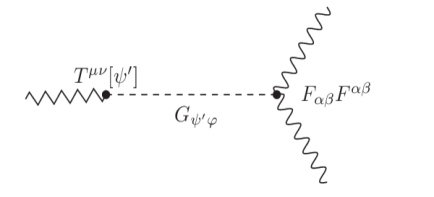
Figure 7: Tree Diagram of the Effective Action (168), which reproduces the trace of the triangle anomaly. The dashed line denotes the propagator $G_{\psi^{\prime}\varphi}=\,\raise 0.5pt\hbox{$\vbox{\hrule\hbox{\vrule height=6.50403pt\kern 6.50403pt\vrule} \hrule}$}\,^{-1}$ of the scalar intermediate state, while the jagged line denotes the gravitational metric field variation $h_{\mu\nu}=\delta g_{\mu\nu}$. Compare to Fig. 6

The massless degrees of freedom $\varphi$ and $\psi^{\prime}$ are a necessary consequence of the trace anomaly, required by imposition of all the other symmetries. In this case these are scalar rather than pseudoscalar degrees of freedom. An important physical difference with the axial case is that the introduction in QED of a chiral current $J_{5}^{\mu}$ and axial vector source ${\cal B}_{\mu}$ corresponding to it appear rather artificial, and difficult to realize in Nature, whereas the trace of the stress tensor obtained by a conformal variation of the effective action is simply a particular metric variation already present in the QED Lagrangian in curved space, required by general coordinate invariance and the Equivalence Principle, without any additional couplings or extraneous fields. Since the stress-energy tensor couples to the universal force of gravity, we should expect that physical processes can excite the scalar $\varphi$ and $\psi^{\prime}$ scalar degrees of freedom required by the trace anomaly with a gravitational coupling strength, which can produce effects of arbitrarily long range.

IV.6 The Scalar Anomaly Pole and Gravitational Scattering Amplitudes

In order to verify the existence of the massless scalar pole in a physical process, consider the simple tree diagram of gravitational exchange between an arbitrary conserved stress-energy source $T^{\prime\,\mu\nu}$ and photons illustrated in Fig. 8.

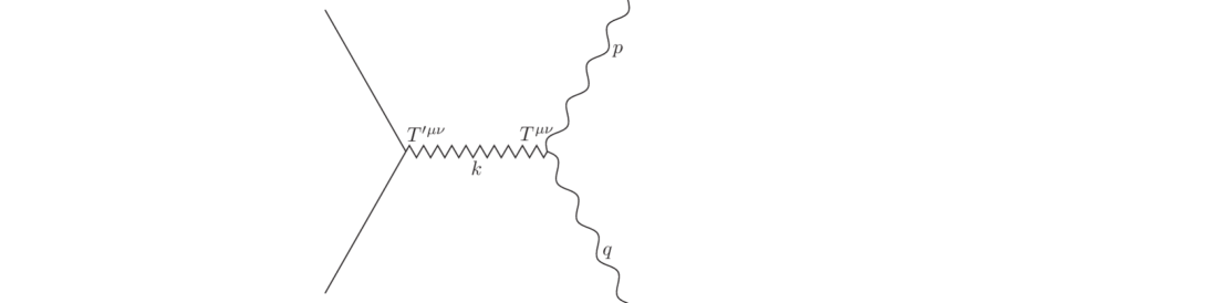
Figure 8: Tree Level Gravitational Scattering Amplitude

This process is described by the scattering amplitude Feyn ,

$${\cal M}=8\pi G\int d^{4}x^{\prime}\int d^{4}x\,\left[T^{\prime\,\mu\nu}(x^{\prime})\,\left(\frac{\hskip 1.42271pt1}{\,\raise 0.5pt\hbox{$\vbox{\hrule\hbox{\vrule height=6.50403pt\kern 6.50403pt\vrule} \hrule}$}\,}\right)_{x^{\prime},x}T_{\mu\nu}(x)-\frac{1}{2}\,T^{\prime\,\mu}_{\ \ \mu}(x^{\prime})\,\left(\frac{\hskip 1.42271pt1}{\,\raise 0.5pt\hbox{$\vbox{\hrule\hbox{\vrule height=6.50403pt\kern 6.50403pt\vrule} \hrule}$}\,}\right)_{x^{\prime},x}T^{\nu}_{\ \nu}(x)\right].$$ (174)

The relative factor of $-\frac{1}{2}$ between the two terms is dictated by the requirement that there be no scalar or ghost state exchanged between the two sources, and is exactly the prediction of General Relativity, linearized about flat space. That only a spin-$2$ propagating degree of freedom is exchanged between the two sources in Fig. 8 can be verified by introducing the following $3+1$ decomposition for each of the conserved stress tensors,

$$T^{00}=T_{00}\,,$$ (175a)

$$T^{0i}=-V^{\perp\,i}-\partial^{i}\frac{1\hskip 2.84544pt}{\nabla^{2}}\,\dot{T}_{00}\,,$$ (175b)

$$T^{ij}=T^{\perp\,ij}+\partial^{i}\frac{1\hskip 2.84544pt}{\nabla^{2}}\,\dot{V}^{\perp\,j}+\partial^{j}\frac{1\hskip 2.84544pt}{\nabla^{2}}\,\dot{V}^{\perp\,i}+\frac{1}{2}\left(g^{ij}-\partial^{i}\frac{1\hskip 2.84544pt}{\nabla^{2}}\,\partial^{j}\right)(T^{\mu}_{\ \mu}+T_{00})$$

$$\qquad\qquad-\frac{1}{2}\left(g^{ij}-3\,\partial^{i}\frac{1\hskip 2.84544pt}{\nabla^{2}}\,\partial^{j}\right)\frac{1\hskip 2.84526pt}{\nabla^{2}}\,\ddot{T}_{00}\,,$$ (175c)

where $\partial_{i}V^{\perp\,i}=0$, $\partial_{i}T^{\perp\,ij}=T^{\perp\,i}_{\ i}=0$, and $\nabla^{-2}$ denotes the static Green’s function of the Laplacian operator, $\nabla^{2}=\partial^{i}\partial_{i}$ in flat space. This parameterization assumes only the conservation of the stress-tensor source(s), i.e. $\partial_{\mu}T^{\mu\nu}=0$, so that there remain six independent components of $T^{\mu\nu}$ which must be specified, and we have chosen these six to be $T_{00},V^{\perp\,i},T^{\perp\,ij}$ and the total trace $T^{\mu}_{\ \mu}$, which is a spacetime scalar. Substituting the decomposition (175) into (174) gives

$${\cal M}=8\pi G\int d^{4}x^{\prime}\int d^{4}x\,\left[T^{\prime\perp}_{ij}\left(\frac{1}{\,\raise 0.5pt\hbox{$\vbox{\hrule\hbox{\vrule height=6.50403pt\kern 6.50403pt\vrule} \hrule}$}\,}\right)_{x^{\prime},x}T^{\perp}_{ij}-2\,V^{\prime\perp}_{i}\left(\frac{1\hskip 2.84544pt}{\nabla^{2}}\right)_{x^{\prime},x}V^{\perp}_{i}\right.$$

$$\left.+\frac{3}{2}\,T^{\prime}_{00}\frac{1\hskip 5.69046pt}{(\nabla^{2})^{2}}_{x^{\prime},x}\,\raise 0.5pt\hbox{$\vbox{\hrule\hbox{\vrule height=6.50403pt\kern 6.50403pt\vrule} \hrule}$}\,\,T_{00}+\frac{1}{2}\,T^{\prime}_{00}\left(\frac{1\hskip 2.84544pt}{\nabla^{2}}\right)_{x^{\prime},x}\,T^{\mu}_{\ \mu}+\frac{1}{2}\,T^{\prime\mu}_{\ \ \mu}\,\left(\frac{1\hskip 2.84544pt}{\nabla^{2}}\right)_{x^{\prime},x}T_{00}\right]\,,$$ (176)

which becomes the five terms

$${\cal M}\rightarrow-8\pi G\left[T^{\prime\perp}_{ij}\frac{1}{k^{2}}\,T^{\perp}_{ij}\,-2\,V^{\prime\perp}_{i}\,\frac{1}{\vec{k}^{2}}\,V^{\perp}_{i}+\frac{3}{2}\,T^{\prime}_{00}\,\frac{k^{2}}{(\vec{k}^{2})^{2}}\,\,T_{00}+\frac{1}{2}T^{\prime}_{00}\,\frac{1}{\vec{k}^{2}}\,T^{\mu}_{\ \mu}+\frac{1}{2}\,T^{\prime\mu}_{\ \ \mu}\,\frac{1}{\vec{k}^{2}}\,T_{00}\right]$$ (177)

in momentum space. These expressions show that only the spatially transverse and tracefree components of the stress tensor, $T^{\perp}_{ij}$ exchange a physical propagating helicity $\pm 2$ graviton in the intermediate state, characterized by a Feynman (or for classical interactions, a retarded) massless propagator $-\,\raise 0.5pt\hbox{$\vbox{\hrule\hbox{\vrule height=6.50403pt\kern 6.50403pt\vrule} \hrule}$}\,^{-1}\rightarrow k^{-2}$ pole in the first term of (176) or (177). All the other four terms in either expression contain only an instantaneous Coulomb-like interaction $-\nabla^{-2}\rightarrow\vec{k}^{-2}$ or $\nabla^{-4}\rightarrow\vec{k}^{-4}$ between the sources, in which no propagating physical particle appears in the intermediate state of the cut diagram. This is the gravitational analog of the decomposition,

$$J^{0}=\rho\,,$$ (178a)

$$J^{i}=J^{\perp\,i}-\partial^{i}\frac{1\hskip 2.84544pt}{\nabla^{2}}\,\dot{\rho}\,,$$ (178b)

of the conserved electromagnetic current and corresponding tree level scattering amplitude,

$$\int\!d^{4}x^{\prime}\!\int\!\!d^{4}x\,J^{\prime\mu}(x^{\prime})\!\left(\frac{1}{\,\raise 0.5pt\hbox{$\vbox{\hrule\hbox{\vrule height=6.50403pt\kern 6.50403pt\vrule} \hrule}$}\,}\right)_{x^{\prime},x}J_{\mu}(x)\rightarrow-J^{\prime\mu}\frac{1}{k^{2}}J_{\mu}=-J^{\prime\perp}_{i}\,\frac{1}{k^{2}}\,J^{\perp}_{i}+\rho^{\prime}\,\frac{1}{\vec{k}^{2}}\,\rho\,,$$ (179)

which shows that only a helicity $\pm 1$ photon is exchanged between the transverse components of the current, the last term in (179) being the instantaneous Coulomb interaction between the charge densities.

We now replace one of the stress tensor sources by the matrix element of the one-loop anomalous amplitude, considering first the trace term with the anomaly pole in $F_{1}$. This corresponds to the diagram in Fig. 9. We find for this term,

$$\langle 0|T_{00}|p,q\rangle_{{}_{1}}=-\vec{k}^{2}F_{1}(k^{2})\,u^{\alpha\beta}(p,q)\tilde{A}_{\alpha}(p)\tilde{A}_{\beta}(q)\,$$ (180a)

$$\langle 0|T^{\mu}_{\ \mu}|p,q\rangle_{{}_{1}}=3k^{2}F_{1}(k^{2})\,u^{\alpha\beta}(p,q)\tilde{A}_{\alpha}(p)\tilde{A}_{\beta}(q)\,$$ (180b)

$$\langle 0|V^{\perp}_{i}|p,q\rangle_{{}_{1}}=\langle 0|T^{\perp}_{ij}|p,q\rangle_{{}_{1}}=0\,.$$ (180c)

Hence the scattering amplitude (177) becomes simply,

$${\cal M}_{1}=4\pi G\,T^{\prime\mu}_{\ \ \mu}\,F_{1}(k^{2})\,u^{\alpha\beta}(p,q)\tilde{A}_{\alpha}(p)\tilde{A}_{\beta}(q)=\frac{4\pi G}{3}\,T^{\prime\mu}_{\ \ \mu}\,\frac{1}{k^{2}}\,\langle 0|T^{\nu}_{\ \nu}|p,q\rangle_{{}_{1}}\,$$ (181)

where (144) has been used for $m=0$. Thus for massless fermions the pole in the anomaly amplitude becomes a scalar pole in the gravitational scattering amplitude, appearing in the intermediate state as a massless scalar exchange between the traces of the energy-momentum tensors on each side. The standard gravitational interaction with the source has produced an effective interaction between the scalar auxiliary field $\psi^{\prime}$ and the trace $T^{\prime\mu}_{\ \ \mu}$ with a well defined gravitational coupling. Thus we may equally well represent the scattering as Fig. 9 involving the fermion triangle, or as the tree level diagram Fig. 10 of the effective theory, with a massless scalar exchange.

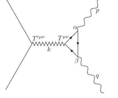
Figure 9: Gravitational Scattering of photons from the source $T^{\prime\mu\nu}$ via the triangle amplitude

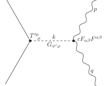
Figure 10: Gravitational scattering of photons from the trace of a source $T^{\prime\mu}_{\ \ \mu}$ via massless scalar exchange in the effective theory of (182).

This tree diagram is generated by the effective action in flat space modified from (168) to

$$S_{eff}[g,A;\varphi,\psi^{\prime}]=\int\,d^{4}x\,\sqrt{-g}\left[-\psi^{\prime}\,\raise 0.5pt\hbox{$\vbox{\hrule\hbox{\vrule height=6.50403pt\kern 6.50403pt\vrule} \hrule}$}\,\,\varphi+\frac{8\pi G}{3}\,T^{\prime\mu}_{\ \ \mu}\,\psi^{\prime}+\frac{c}{2}\,F_{\alpha\beta}F^{\alpha\beta}\varphi\right],$$ (182)

to include the coupling to the trace of the energy-momentum tensor of any matter $T^{\prime\mu}_{\ \ \mu}$ source. Correspondingly the eq. (169c) for $\varphi$ becomes

$$\,\raise 0.5pt\hbox{$\vbox{\hrule\hbox{\vrule height=6.50403pt\kern 6.50403pt\vrule} \hrule}$}\,\varphi=\frac{8\pi G}{3}\,T^{\prime\mu}_{\ \ \mu}\,,$$ (183)

instead of (169c). The eq. of motion for $\psi^{\prime}$ remains (169b). We note that if the source $T^{\prime\mu\nu}$ generates the curvature $R$ by Einstein’s eqs., then $R=-8\pi G\,T^{\prime\mu}_{\ \ \mu}$, so that (182) and (183) are equivalent to (168) and (169c) at leading order in $G$.

We conclude that in the conformal limit of massless electrons, the pole in the trace sector of the $\langle TJJ\rangle$ anomaly amplitude contributes to gravitational scattering amplitudes as would a scalar field coupled to the trace of the energy-momentum tensor of classical sources. The gravitationally coupled intermediate scalar can be understood as arising from collinear $e^{+}e^{-}$ correlated pairs in a total spin $0^{+}$ state in Fig. 6. Although the result appears similar in some respects to a Brans-Dicke scalar JBD , and indeed (183) is identical in form to that of a Brans-Dicke scalar with vanishing Brans-Dicke coupling ($\omega=0$), because of the unusual off-diagonal kinetic term dictated by the structure of the trace anomaly, (182) is certainly not a Brans-Dicke theory. Thus, although (183) tells us that $\varphi$ is sourced by the trace of matter stress tensor with gravitational strength, $\varphi$ cannot react back on matter except through $\psi^{\prime}$ and hence $F_{\alpha\beta}F^{\alpha\beta}$, reproducing (167), from whence it was derived. Each of the two scalar fields each couples to a different source, with an off-diagonal propagator, $G_{\psi^{\prime}\varphi}$. There is no direct coupling of the trace of matter stress tensors $T^{\prime\mu}_{\ \mu}$ to $T^{\nu}_{\ \nu}$ via a scalar exchange as there would be in a classical scalar tensor theory of the Jordan-Brans-Dicke kind. Hence the phenomenology of (182) will be quite different, and the observational limits on a Jordan-Brans-Dicke scalar Will do not apply. Note also that the matrix elements of $F_{\alpha\beta}F^{\alpha\beta}=2(\vec{E}^{2}-\vec{B}^{2})$ vanish for monochromatic photons on shell. Thus to leading order the scattering diagram in Fig. 9 also does not contribute to photon scattering on shell. The contribution of the massless scalar pole to higher order or off shell physical processes and the prospects for detecting its effects experimentally are important and interesting questions currently under investigation.

IV.7 The Effective Action of Low Energy Gravity

With the foregoing detailed consideration of anomalies, massless poles and their long distance effects, we consider finally the EFT of four dimensional macroscopic gravity. This gravitational EFT is determined by the same general principles as in other contexts DGH , namely by an expansion in powers of derivatives of local terms consistent with symmetry. Short distance effects are parameterized by the coefficients of local operators in the effective action, with higher order terms suppressed by inverse powers of an ultraviolet cutoff scale $M_{{}_{UV}}$. The effective theory need not be renormalizable, as indeed Einstein’s theory is not, but is expected nonetheless to be quite insensitive to the details of the underlying microscopic degrees of freedom, because of decoupling DGH . It is the decoupling of short distance degrees of freedom from the macroscopic physics that makes EFT techniques so widely applicable, and which we assume applies also to gravity.

As a covariant metric theory with a symmetry dictated by the Equivalence Principle, General Relativity may be regarded as just such a local EFT, truncated at second order in derivatives of the metric field $g_{ab}(x)$ Dono . When quantum matter is considered, the stress tensor $T^{a}_{\ b}$ becomes an operator. Because the stress tensor has mass dimension four, containing up to quartic divergences, the proper covariant renormalization of this operator requires fourth order terms in derivatives of the metric. However the effects of such higher derivative local terms in the gravitational effective action are suppressed at distance scales $L\gg L_{Pl}$ in the low energy EFT limit. Hence surveying only local curvature terms, it is often tacitly assumed that Einstein’s theory contains all the low energy macroscopic degrees of freedom of gravity, and that General Relativity cannot be modified at macroscopic distance scales, much greater than $L_{Pl}$, without violating general coordinate invariance and/or EFT principles. As we have argued previously in two dimensions, this presumption should be re-examined in the presence of quantum anomalies.

When a classical symmetry is broken by a quantum anomaly, the naive decoupling of short and long distance physics assumed by an expansion in local operators with ascending inverse powers of $M_{{}_{UV}}$ fails. In this situation even the low energy symmetries of the effective theory are changed by the presence of the anomaly, and some remnant of the ultraviolet physics survives in the low energy description. An anomaly can have significant effects in the low energy EFT because it is not suppressed by any large energy cutoff scale, surviving even in the limit $M_{{}_{UV}}\rightarrow\infty$. Any explicit breaking of the symmetry in the classical Lagrangian serves only to mask the effects of the anomaly, but in the right circumstances the effects of the non-local anomaly may still dominate the local terms. The axial anomaly in QCD, discussed in Sec. IV.1 has low energy effects, unsuppressed by the EFT ultraviolet cutoff scale, $M_{{}_{UV}}\sim\Lambda_{QCD}$ in that case. Although the quark masses are non-zero, and chiral symmetry is only approximate in Nature, the chiral anomaly gives the dominant contribution to the low energy decay amplitude of $\pi^{0}\rightarrow 2\gamma$ in the standard model Adler ; BarFriGM , a contribution that is missed entirely by a local EFT expansion in pion fields. Instead the existence of the chiral anomaly requires the explicit addition to the local effective action of a non-local term in four physical dimensions to account for its effects WZ ; DGH . Although when an anomaly is present, naive decoupling between the short and long distance degrees of freedom fails, it does so in a well-defined way, with a coefficient that depends only on the quantum numbers of the underlying microscopic theory.

The low energy effective action for gravity in four dimensions contains first of all, the local terms constructed from the Riemann curvature tensor and its derivatives and contractions up to and including dimension four. This includes the usual Einstein-Hilbert action of General Relativity,

$$S_{EH}[g]=\frac{1}{16\pi G}\int\,d^{4}x\,\sqrt{-g}\,(R-2\Lambda)$$ (184)

as well as the spacetime integrals of the fourth order curvature invariants,

$$S_{local}^{(4)}[g]=\frac{1}{2}\int\,d^{4}x\,\sqrt{-g}\,\left(\alpha C_{abcd}C^{abcd}+\beta R^{2}\right),$$ (185)

with arbitrary dimensionless coefficients $\alpha$ and $\beta$. There are two additional fourth order invariants, namely $E=^{*}\hskip-5.69046ptR_{abcd}\,^{*}\hskip-2.84544ptR^{abcd}$ and $\,\raise 0.5pt\hbox{$\vbox{\hrule\hbox{\vrule height=6.50403pt\kern 6.50403pt\vrule} \hrule}$}\,R$, which could be added to (185) as well, but as they are total derivatives yielding only a surface term and no local variation, we omit them. All the possible local terms in the effective action may be written as the sum,

$$S_{local}[g]=\frac{1}{16\pi G}\int\,d^{4}x\,\sqrt{-g}\,(R-2\Lambda)+S_{local}^{(4)}+\sum_{n=3}^{\infty}S_{local}^{(2n)}\,.$$ (186)

with the terms in the sum with $n\geq 3$ composed of integrals of local curvature invariants with dimension $2n\geq 6$, and suppressed by $M_{{}_{UV}}^{-2n+4}$ at energies much less than $M_{{}_{UV}}$. Here $M_{{}_{UV}}$ is the ultraviolet cutoff scale of the low energy effective theory which we may take to be of order $M_{pl}$. The higher derivative terms with $n\geq 3$ are irrelevant operators in the infrared, scaling with negative powers under global rescalings of the metric, and may be neglected at macroscopic distance scales, at least with respect to the classical scaling dimensions. On the other hand the two terms in the Einstein-Hilbert action $n=0,1$ scale positively, and are clearly relevant in the infrared. The fourth order terms in (185) are neutral under such global rescalings.

The exact quantum effective action also contains non-local terms in general. All possible terms in the effective action (local or not) can be classified according to how they respond to global Weyl rescalings of the metric, i.e. $\sigma=\sigma_{0}=$ const. If the non-local terms are non-invariant under global rescalings, then they scale either positively or negatively under (146). If $m^{-1}$ is some fixed length scale associated with the non-locality, arising for example by the integrating out of fluctuations of fields with mass $m$, then at much larger macroscopic distances ($mL\gg 1$) the non-local terms in the effective action become approximately local. The terms which scale with positive powers of $e^{\sigma_{0}}$ are constrained by general covariance to be of the same form as the $n=0,1$ Einstein-Hilbert terms in $S_{local}$, (184). Terms which scale negatively with $e^{\sigma_{0}}$ become negligibly small as $mL\gg 1$ and are infrared irrelevant at macroscopic distances. This is the expected decoupling of short distance degrees of freedom in an effective field theory description, which are verified in detailed calculations of loops in massive field theories in curved space. The only possibility for contributions to the effective field theory of gravity at macroscopic distances, which are not contained in the local expansion of (186) arise from fluctuations not associated with any finite length scale, i.e. $m=0$. These are the non-local contributions to the low energy EFT which include those associated with the anomaly.

The anomaly effective action is associated with non-trivial cohomology of the Weyl group in the space of metrics. Since $\Gamma_{WZ}$ (161) from which the effective action of the anomaly was derived satisfies WZ consistency, i.e. is closed but not exact under the Weyl group, it is unique up to an arbitrary admixture of local trivial cocycles, which in physical terms are either trivial because they are completely Weyl invariant effective actions obeying

$$S_{inv}[e^{2\sigma}g]=S_{inv}[g]\,,$$ (187)

and drop out of difference (162), or they are purely local terms easily catalogued by ascending powers of the Riemann curvature tensor, its covariant derivatives and contractions in (186). Thus the classification of terms according to their global Weyl scaling properties tells us that the exact effective action of any covariant theory must be of the form MazMot ,

$$S_{exact}[g]=S_{local}[g]+S_{inv}[g]+S_{anom}[g]\,,$$ (188)

with $S_{local}$ given by the expansion (186), $S_{inv}$ the (generally non-local) Weyl invaraint terms satisfying (187), and $S_{anom}$ the anomaly action given by (165)-(166). The higher dimension local terms in (186) are strictly irrelevant in the IR, since they scale to zero with negative powers of $e^{\sigma_{0}}$ and may be neglected for physics far below the Planck scale, while the lower dimension local terms are nothing but the terms of the usual Einstein-Hilbert classical action (184). These classical terms grow as positive powers of $e^{\sigma_{0}}$ under global dilations and are clearly IR relevant terms. Indeed the naive classical scaling of these terms are positive powers ($L^{4}$ and $L^{2}$) under rescaling of distance, and are clearly relevant operators of the low energy description.

The local dimension four terms involving the Weyl tensor squared $C^{2}$ is fully locally Weyl invariant (while that involving $R^{2}$ is invariant only under global Weyl rescalings) and among the many terms that can appear in $S_{inv}$. Because both of these are neutral under global dilations, scaling like $L^{0}$ we expect them to be marginally irrelevant in the IR (as well as in the UV). All the higher dimension local terms in the sum in (186) for $n\geq 3$ scale to zero as $\sigma_{0}\rightarrow\infty$ and are clearly strictly IR irrelevant. However among all the possible terms that can be generated by quantum loops in the exact effective action of gravity, the anomaly effective action is unique in scaling logarithmically under the global Weyl group. Indeed we note that in the form (166) the simple shift of the auxiliary field $\varphi$ by a spacetime constant,

$$\varphi\rightarrow\varphi+2\sigma_{0}$$ (189)

corresponding to a global logarithmic variation of length scales yields the entire dependence of $S_{anom}$ on the global Weyl rescalings (146), viz.

$$S_{anom}[g;\varphi,\psi]\rightarrow S_{anom}[e^{2\sigma_{0}}g;\varphi+2\sigma_{0},\psi]$$

$$\quad=S_{anom}[g;\varphi,\psi]+\sigma_{0}\!\,\int\,d^{4}x\,\sqrt{-g}\left[bF+b^{\prime}\left(E-\frac{2}{3}\,\raise 0.5pt\hbox{$\vbox{\hrule\hbox{\vrule height=6.50403pt\kern 6.50403pt\vrule} \hrule}$}\,R\right)\right],\qquad\quad$$ (190)

owing to the strict invariance of the terms quadratic in the auxiliary fields under (146) and eqs. (158). Hence $S_{anom}$ scales logarithmically ($\sim\log L$) with distance under Weyl rescalings.

Because of this infrared sensitivity to global rescalings, unlike local higher derivative terms in the effective action, which are either neutral or scale with negative powers of $L$, the anomalous terms should not be discarded in the low energy, large distance limit. Ordinarily, i.e. absent anomalies, the Wilson effective action should contain only local infrared relevant terms consistent with symmetry RG . However, like the anomalous effective action generated by the chiral anomaly in QCD, the non-local $S_{anom}$ must be included in the low energy EFT to account for the anomalous Ward identities, even in the zero momentum limit, and indeed logarithmic scaling with distance (190) indicates that $S_{anom}$ is an infrared relevant term. Even if no massless matter fields are assumed, the quantum fluctuations of the metric itself will generate a term of the same form as $S_{anom}$ in the infrared AMMc . The scalar fields of the local form (165)-(166) of $S_{anom}$ describe massless scalar degrees of freedom of low energy gravity, not contained in classical General Relativity. As we have seen, these massless scalars may be understood as correlated two-particle states of the underlying anomalous QFT, and show up as poles in gauge invariant physical scattering amplitudes in the EFT where the original quantum fields appear only in internal quantum loops. Thus the effective action of the anomaly $S_{anom}$ should be retained in the EFT of low energy gravity, which is specified then by the first two strictly relevant local terms of the classical Einstein-Hilbert action (184), and the logarithmic $S_{anom}$, i.e.

$$S_{eff}[g]=S_{{}_{EH}}[g]+S_{anom}[g;\varphi,\psi]$$ (191)

with $S_{anom}$ is given by (163) or in its local form by (165)-(166).

The complete classification of the terms in the exact effective action (188) into just three categories means that all possible infrared relevant terms in the low energy EFT, which are not contained in $S_{local}$ of (186) must fall into $S_{anom}$, i.e. they must correspond to non-trivial co-cycles of the local Weyl group MazMot ; MotVau . The Weyl invariant terms in the exact effective action (187) are by definition insensitive to rescaling of the metric at large distances. Hence the (generally quite non-local) terms in $S_{inv}$ do not give rise to infrared relevant terms in the Wilson effective action for low energy gravity. By this classification of terms (local or non-local) according to their behavior under global Weyl rescalings, the Wilson effective action (191) contains all the infrared relevant terms in low energy gravity for energies much less than $M_{pl}$.

Note also that it would be inconsistent with the semi-classical Einstein eqs. (42) to have as their source a stress tensor which is not covariantly conserved. Thus in a clash of symmetries which a quantum anomaly presents, it is necessary to choose the option that conformal invariance is broken, not general coordinate invariance. The action $S_{anom}$ is invariant under general coordinate transformations and under no conditions (i.e. in the presence of an horizon or not) is there a gravitational anomaly Bertl . This is not a state dependent condition dependent on whether an horizon exists or not, but a condition of consistency of the semi-classical Einstein eqs. (42). Under the defining assumptions of general covariance and the EFT hypothesis of decoupling of physics associated with massive degrees of freedom, any infrared modifications of Einstein’s theory generated by quantum effects is tightly constrained and the effective action (191) becomes essentially unique. The addition of the anomaly term(s) and the scalar degrees of freedom $\varphi$ and $\psi$ they contain to the low energy effective action of gravity amounts to a non-trivial infrared modification of General Relativity, required by the existence of the trace anomaly, fully consistent with both quantum theory and the Equivalence Principle.

V Macroscopic Effects of the Trace Anomaly

Having a fully covariant effective action the most straightforward application is to compute the covariantly conserved stress-energy tensor corresponding to it, and study its effects in particular backgrounds. If the effects are significant it will be necessary then to include the anomalous stress tensor as a source for Einstein’s eqs. to obtain new solutions, but at first one can evauate the stress tensor in certain fixed backgrounds, such as the Schwarzschild black hole geometry discussed in Sec. II and the de Sitter geometry of Sec. III. This will provide the first evidence of the relevance of the anomaly effective action and the scalars $\varphi$ and $\psi$ for macroscopic gravity in the presence of horizons.

After these studies in fixed classical backgrounds one can consider next dynamical effects of the fluctuations associated with the anomaly scalars, their role in cosmology and their relevance to both the problem of gravitational collapse and cosmological dark energy.

V.1 Anomaly Stress Tensor in Schwarzschild Spacetime

From (165) and (166) the stress tensor of the anomalous effective action consists of two independent terms,

$$T_{ab}^{(anom)}\equiv-\frac{2}{\sqrt{-g}}\frac{\delta S_{anom}}{\delta g^{ab}}[g;\varphi,\psi]=b^{\prime}E_{ab}+bF_{ab}$$ (192)

namely

$$E_{ab} = -2\,(\nabla_{(a}\varphi)(\nabla_{b)}\,\raise 0.5pt\hbox{$\vbox{\hrule\hbox{\vrule height=6.50403pt\kern 6.50403pt\vrule} \hrule}$}\,\varphi)+2\,\nabla^{c}\left[(\nabla_{c}\varphi)(\nabla_{a}\nabla_{b}\varphi)\right]-\frac{2}{3}\,\nabla_{a}\nabla_{b}\left[(\nabla_{c}\varphi)(\nabla^{c}\varphi)\right]$$ (193)

$$+\frac{2}{3}\,R_{ab}\,(\nabla_{c}\varphi)(\nabla^{c}\varphi)-4\,R^{c}_{\ (a}(\nabla_{b)}\varphi)(\nabla_{c}\varphi)+\frac{2}{3}\,R\,(\nabla_{a}\varphi)(\nabla_{b}\varphi)$$

$$+\frac{1}{6}\,g_{ab}\,\left\{-3\,(\,\raise 0.5pt\hbox{$\vbox{\hrule\hbox{\vrule height=6.50403pt\kern 6.50403pt\vrule} \hrule}$}\,\varphi)^{2}+\,\raise 0.5pt\hbox{$\vbox{\hrule\hbox{\vrule height=6.50403pt\kern 6.50403pt\vrule} \hrule}$}\,\left[(\nabla_{c}\varphi)(\nabla^{c}\varphi)\right]+2\left(3R^{cd}-Rg^{cd}\right)(\nabla_{c}\varphi)(\nabla_{d}\varphi)\right\}$$

$$-\frac{2}{3}\,\nabla_{a}\nabla_{b}\,\raise 0.5pt\hbox{$\vbox{\hrule\hbox{\vrule height=6.50403pt\kern 6.50403pt\vrule} \hrule}$}\,\varphi-4\,C_{a\ b}^{\ c\ d}\,\nabla_{c}\nabla_{d}\varphi-4\,R_{(a}^{c}\nabla_{b)}\nabla_{c}\varphi+\frac{8}{3}\,R_{ab}\,\,\raise 0.5pt\hbox{$\vbox{\hrule\hbox{\vrule height=6.50403pt\kern 6.50403pt\vrule} \hrule}$}\,\varphi+\frac{4}{3}\,R\,\nabla_{a}\nabla_{b}\varphi$$

$$-\frac{2}{3}\!\left(\nabla_{(a}R\right)\nabla_{b)}\varphi+\frac{1}{3}g_{ab}\left\{2\,\raise 0.5pt\hbox{$\vbox{\hrule\hbox{\vrule height=6.50403pt\kern 6.50403pt\vrule} \hrule}$}\,^{2}\varphi+6R^{cd}\,\nabla_{c}\nabla_{d}\varphi-4R\,\raise 0.5pt\hbox{$\vbox{\hrule\hbox{\vrule height=6.50403pt\kern 6.50403pt\vrule} \hrule}$}\,\varphi+(\nabla^{c}R)\nabla_{c}\varphi\right\}$$

and

$$F_{ab}\!=\!-2(\nabla_{(a}\varphi)(\nabla_{b)}\!\,\raise 0.5pt\hbox{$\vbox{\hrule\hbox{\vrule height=6.50403pt\kern 6.50403pt\vrule} \hrule}$}\,\psi)\!-\!2(\nabla_{(a}\psi)(\nabla_{b)}\!\,\raise 0.5pt\hbox{$\vbox{\hrule\hbox{\vrule height=6.50403pt\kern 6.50403pt\vrule} \hrule}$}\,\varphi)\!+\!2\nabla^{c}\!\left[(\nabla_{c}\varphi)(\nabla_{a}\!\nabla_{b}\psi)\!+\!(\nabla_{c}\psi)(\nabla_{a}\!\nabla_{b}\varphi)\right]$$

$$-\frac{4}{3}\nabla_{a}\nabla_{b}\left[(\nabla_{c}\varphi)(\nabla^{c}\psi)\right]+\frac{4}{3}R_{ab}(\nabla_{c}\varphi)(\nabla^{c}\psi)-4R^{c}_{\ (a}\!\left[(\nabla_{b)}\varphi)(\nabla_{c}\psi)\!+\!(\nabla_{b)}\psi)(\nabla_{c}\varphi)\right]$$

$$\hskip 28.45274pt+\frac{4}{3}R\,(\nabla_{(a}\varphi)(\nabla_{b)}\psi)+\frac{1}{3}g_{ab}\Big{\{}-3(\,\raise 0.5pt\hbox{$\vbox{\hrule\hbox{\vrule height=6.50403pt\kern 6.50403pt\vrule} \hrule}$}\,\varphi)(\,\raise 0.5pt\hbox{$\vbox{\hrule\hbox{\vrule height=6.50403pt\kern 6.50403pt\vrule} \hrule}$}\,\psi)+\,\raise 0.5pt\hbox{$\vbox{\hrule\hbox{\vrule height=6.50403pt\kern 6.50403pt\vrule} \hrule}$}\,\left[(\nabla_{c}\varphi)(\nabla^{c}\psi)\right]$$

$$\hskip 8.5359pt\left.+2\left(3R^{cd}-Rg^{cd}\right)(\nabla_{c}\varphi)(\nabla_{d}\psi)\right\}-4\,\nabla_{c}\nabla_{d}\left(C_{(a\ b)}^{\ \ c\ \ d}\varphi\right)-2\,C_{a\ b}^{\ c\ d}R^{cd}\varphi$$

$$-\frac{2}{3}\,\nabla_{a}\nabla_{b}\,\raise 0.5pt\hbox{$\vbox{\hrule\hbox{\vrule height=6.50403pt\kern 6.50403pt\vrule} \hrule}$}\,\psi-4\,C_{a\ b}^{\ c\ d}\,\nabla_{c}\nabla_{d}\psi-4\,R_{(a}^{c}(\nabla_{b)}\nabla_{c}\psi)+\frac{8}{3}\,R_{ab}\,\,\raise 0.5pt\hbox{$\vbox{\hrule\hbox{\vrule height=6.50403pt\kern 6.50403pt\vrule} \hrule}$}\,\psi+\frac{4}{3}\,R\,\nabla_{a}\nabla_{b}\psi$$

$$-\frac{2}{3}\!\left(\nabla_{(a}R\right)\nabla_{b)}\psi+\frac{1}{3}g_{ab}\left\{\!2\,\raise 0.5pt\hbox{$\vbox{\hrule\hbox{\vrule height=6.50403pt\kern 6.50403pt\vrule} \hrule}$}\,^{2}\psi+6R^{cd}\,\nabla_{c}\nabla_{d}\psi-4R\,\raise 0.5pt\hbox{$\vbox{\hrule\hbox{\vrule height=6.50403pt\kern 6.50403pt\vrule} \hrule}$}\,\psi+(\nabla^{c}R)(\nabla_{c}\psi)\!\right\}.$$ (194)

Each of these two tensors are individually conserved and they have the local traces,

$$E^{a}_{\ a} = 2\Delta_{4}\varphi=E-\frac{2}{3}\,\raise 0.5pt\hbox{$\vbox{\hrule\hbox{\vrule height=6.50403pt\kern 6.50403pt\vrule} \hrule}$}\,R\,,$$ (195a)

$$F^{a}_{\ a} = 2\Delta_{4}\psi=F=C_{abcd}C^{abcd}\,,$$ (195b)

corresponding to the two terms respectively in the trace anomaly in four dimensions in (155) (with $\beta_{i}=0$).

In the four dimensional Schwarzschild geometry the full contraction of the Riemann tensor is given by (6), and since $R_{ab}=0$ the invariants $F\big{|}_{{}_{S}}=E\big{|}_{{}_{S}}={48\,M^{2}}/{r^{6}}$. (where we temporarily set $GM=M$ to simplify the expressions below). A particular solution of either of the inhomogeneous Eqs. (164) is given then by $\bar{\varphi}(r)$, with

$$\frac{d\bar{\varphi}}{dr}\Big{|}_{{}_{S}}=-\frac{4M}{3r^{2}f}\ln\left(\frac{r}{2M}\right)-\frac{1}{2M}\left(1+\frac{4M}{r}\right)$$ (196)

and $f(r)=1-\frac{2M}{r}$, The general solution of (164) for $\varphi=\varphi(r)$ away from the singular points $r=(0,2M,\infty)$ is easily found and may be expressed in the form

$$\frac{d\varphi}{dr}\Big{|}_{{}_{S}}=\frac{d\bar{\varphi}}{dr}\Big{|}_{{}_{S}}+\frac{2Mc_{{}_{H}}}{r^{2}f}+\frac{q-2}{4M^{2}r^{2}f}\!\int_{2M}^{r}\!drr^{2}\ln f+\frac{c_{\infty}}{2M}\left(\!\frac{r}{2M}+1+\frac{2M}{r}\!\right)$$

$$=\frac{q-2}{6M}\left(\frac{r}{2M}+1+\frac{2M}{r}\right)\ln f-\frac{q}{6r}\left[\frac{4M}{r-2M}\ln\left(\frac{r}{2M}\right)+\frac{r}{2M}+3\right]$$

$$\qquad-\frac{1}{3M}-\frac{1}{r}+\frac{2Mc_{{}_{H}}}{r(r-2M)}+\frac{c_{\infty}}{2M}\,\left(\frac{r}{2M}+1+\frac{2M}{r}\right)$$ (197)

in terms of the three dimensionless constants of integration, $c_{{}_{H}}$, $c_{\infty}$, and $q$. This expression has the limits,

$$\frac{d\varphi}{dr}\Big{|}_{{}_{S}}\!\!\rightarrow\!\frac{c_{{}_{H}}}{r-2M}+\frac{q-2}{2M}\ln\left(\frac{r}{2M}-1\right)-\frac{1}{2M}\!\left(3c_{\infty}-c_{{}_{H}}-q-\frac{5}{3}\right)+\dots,\qquad r\rightarrow 2M;$$ (198a)

$$\frac{d\varphi}{dr}\Big{|}_{{}_{S}}\!\rightarrow\!\frac{c_{\infty}r}{4M^{2}}+\frac{2c_{\infty}-q}{4M}+\frac{c_{\infty}}{r}-\frac{2M}{3r^{2}}\,q\,\ln\left(\frac{r}{2M}\right)+\frac{2M}{r^{2}}\left[c_{{}_{H}}-\frac{7}{18}(q-2)\right]+\dots,\quad r\rightarrow\infty.$$ (198b)

Hence $c_{{}_{H}}$ controls the leading behavior as $r$ approaches the horizon, while $c_{\infty}$ controls the leading behavior as $r\rightarrow\infty$, which is the same as in flat space. The leading behavior at the horizon is determined by the homogeneous solution to (164), $c_{{}_{H}}\ln f=c_{{}_{H}}\ln(-K^{a}K_{a})^{\frac{1}{2}}$ where $K=\partial_{t}$ is the timelike Killing field of the Schwarzschild geometry for $r>2M$. Because of these singular behaviors in (198b), (197) is clearly a solution of (195) in the distributional sense, i.e. containing possible $\delta$ functions or derivatives thereof at the origin, at the horizon and at infinity.

To the general spherically symmetric static solution (197) we may add also a term linear in $t$, i.e. we replace $\varphi(r)$ by

$$\varphi(r,t)=\varphi(r)+\frac{p}{2M}\,t\,.$$ (199)

Linear time dependence in the auxiliary fields is the only allowed time dependence that leads to a time-independent stress-energy. The conformal transformation to flat space near the horizon corresponds to the particular choice $c_{{}_{H}}=\pm p=1$, leaving the subdominant terms in (198a) parameterized by $q$ and $c_{\infty}$ undetermined.

Since the equation for the second auxiliary field $\psi$ is identical to that for $\varphi$, its solution for $\psi=\psi(r,t)$ is of the same form as (197) and (199) with four new integration constants, $d_{{}_{H}},d_{\infty}$, $q^{\prime}$ and $p^{\prime}$ replacing $c_{{}_{H}},c_{\infty}$, $q$, and $p$ in $\varphi(r,t)$. Adding terms with any higher powers of $t$ or more complicated $t$ dependence produces a time dependent stress-energy tensor. Inspection of the stress tensor terms in (192) also shows that it does not depend on either a constant $\varphi_{0}$ or $\psi_{0}$ but only the derivatives of both auxiliary fields in Ricci flat metrics such as Schwarzschild spacetime. For that reason we do not need an additional integration constant for either of the fourth order differential equations (164).

With the general spherically symmetric solution for $\varphi(r,t)$ and $\psi(r,t)$, we can proceed to compute the stress-energy tensor (192) in a stationary, spherically symmetric quantum state. For example the Boulware state is characterized as that state which approaches the flat space vacuum as rapidly as possible as $r\rightarrow\infty$ Boul . In the flat space limit this means that the allowed $r^{2}$ and $r$ behavior in the auxiliary fields ($r$ and constant behavior in their first derivatives) must be set to zero. Inspection of the asymptotic form (198b) shows that this is achieved by requiring

$$c_{\infty}=d_{\infty} = 0\qquad{\rm and}$$ (200a)

$$q=q^{\prime} = 0\,.\qquad{\rm(Boulware)}$$ (200b)

If we set $p=p^{\prime}=0$ as well, in order to have a static ansatz for the Boulware state, then the remaining two constants $c_{{}_{H}}$ and $d_{{}_{H}}$ are free parameters of the auxiliary fields, which lead to a stress-energy which diverges as $r\rightarrow 2M$ on the horizon. Matching the leading divergence of the stress-energy in the Boulware state (41) by adjusting $c_{{}_{H}}$ and $d_{{}_{H}}$ appropriately, one then has a one parameter fit to the numerical data of JenMcOtt . The results of this fit of (192) with $c_{{}_{H}}$ and $d_{{}_{H}}$ treated as free parameters are illustrated in Figs. 11 to 13, for all three non-zero components of the stress tensor expectation value of a massless, conformally coupled scalar field in the Boulware state. The (approximate) best fit values plotted were obtained with $c_{{}_{H}}=-\frac{7}{20}$ and $d_{{}_{H}}=\frac{55}{84}$.

Figure 11: The expectation value $\langle T_{t}^{\ t}\rangle$ of a conformal scalar field in the Boulware state in Schwarzschild spacetime, as a function of $s=\frac{r-2M}{M}$ in units of $\pi^{2}T_{H}^{4}/90$. The solid curve is Eq. (192)-(194) with (196), (197), (200) and $c_{{}_{H}}=-\frac{7}{20},d_{{}_{H}}=\frac{55}{84}$. The dashed curve is the analytic approximation of BroOtt , and the points are the numerical results of JenMcOtt .

Figure 12: The radial pressure $\langle T_{r}^{\ r}\rangle$ of a conformal scalar field in the Boulware state in Schwarzschild spacetime. The axes and solid and dashed curves and points are as in Fig. 11. Note the better agreement of the anomaly stress tensor (solid curve) with the numerical results of JenMcOtt , compared to the analytic approximation of BroOtt .

Figure 13: The tangential pressure $\langle T_{\theta}^{\ \theta}\rangle$ of a conformal scalar field in the Boulware state in Schwarzschild spacetime. The axes and solid and dashed curves and points are as in Fig. 11.

For comparison purposes, we have plotted also the analytic approximation of Page, Brown, and Ottewill BroOtt ; Pag82 ; BrOtP (dashed curves in Figs. 11 to 13). We observe that the two parameter fit with the anomalous stress tensor in terms of the auxiliary $\varphi$ and $\psi$ fields is more accurate than the approximation of refs. BroOtt ; Pag82 ; BrOtP for the Boulware state.

The next important point to emphasize is that the stress-energy diverges on the horizon in an entire family of states for generic values of the eight auxiliary field parameters $(c_{{}_{H}},q,c_{\infty},p;d_{{}_{H}},q^{\prime},d_{\infty},p^{\prime})$, in addition to the Boulware state. Hence in the general allowed parameter space of spherically symmetric macroscopic states, horizon divergences of the stress-energy are quite generic, and not resticted to the Boulware state. On the other hand, the condition that the stress-energy on the horizon be finite gives four conditions on these eight parameters, in order to cancel the four possible divergences $s^{-2},s^{-1},\ln^{2}s,\ln s$. The simplest possibility with the minimal number of conditions on the auxiliary field parameters is via

$$(2b+b^{\prime})c_{{}_{H}}^{2}+p(2bp^{\prime}+b^{\prime}p)=0\qquad(s^{-2})$$ (201a)

$$(b+b^{\prime})c_{{}_{H}}=bd_{{}_{H}}\qquad\qquad(s^{-1})$$ (201b)

$$\qquad q=q^{\prime}=2\qquad\quad(\ln^{2}s\ \ {\rm and}\ \ \ln s)\,.$$ (201c)

It is clear that these finiteness conditions on the horizon are incompatible with the conditions for fall off at infinity (200), in their values of $q$ and $q^{\prime}$. Thus the effective action and behavior of the anomaly scalar fields and stress tensor illustrate at a glance the general topological obstruction discussed in Sec. II for vacuum behavior of $\langle T^{a}_{\ b}\rangle_{{}_{R}}$ at both the horizon and infinity simultaneously. With conditions (200) the anomaly scalar fields give a very weak Casimir-like long-range interaction between massive bodies, that falls off very rapidly with distance (at least as fast as $r^{-7}$).

By taking different values of the parameters $(c_{{}_{H}},q,c_{\infty},p;d_{{}_{H}},q^{\prime},d_{\infty},p^{\prime})$ of the homogeneous solutions to (164), corresponding to different states of the underlying quantum theory, it is possible to approximate the stress tensor of the Hartle-Hawking and Unruh states as well MotVau ; BFS . In states which are regular on the horizon there is no particular reason to neglect the Weyl invariant terms $S_{inv}$ in the exact effective action, and the stress-energy tensor it produces would be expected to be comparable in magnitude to that from $S_{anom}$. In this case of bounded stress tensors, the contributions from both $S_{anom}$ and $S_{inv}$ are both of order $M^{-4}$ and negligibly small on macroscopic scales in any case. However in states such as the previous Boulware example, the diverging behavior of the stress tensor near the horizon is captured accurately by the terms in (192) arising from the anomaly, which have the same generically diverging behaviors as the quantum field theory expectation value $\langle T^{a}_{\ b}\rangle_{{}_{R}}$. This general behavior has been found in the Reissner-Nordstrøm case of electrically charged black holes as well AndMotVau . We find no a priori justification for excluding generic states with stress-energy tensors that grow without bound as the horizon is approached. In any such states the backreaction of the stress-energy on the geometry will be substantial in this region and lead to large backreaction effects near the horizon.

V.2 Anomaly Stress Tensor in de Sitter Spacetime

In conformally flat spacetimes with $g_{ab}=e^{2\sigma}\eta_{ab}$, one can choose $\varphi=2\sigma$ and $\psi=0$ to obtain the stress tensor of the state conformally transformed from the Minkowski vacuum. In this state $F_{ab}$ vanishes, and $\varphi$ can be eliminated completely in terms of the Ricci tensor with the result MazMot ; BroCas ,

$$E_{ab}=\frac{2}{9}\nabla_{a}\nabla_{b}R+2R_{a}^{\ c}R_{bc}-\frac{14}{9}RR_{ab}+g_{ab}\left(-\frac{2}{9}\,\raise 0.5pt\hbox{$\vbox{\hrule\hbox{\vrule height=6.50403pt\kern 6.50403pt\vrule} \hrule}$}\,R-R_{cd}R^{cd}+\frac{5}{9}R^{2}\right)\,.$$ (202)

Thus all non-local dependence on boundary conditions of the auxiliary fields $\varphi$ and $\psi$ drops out in conformally flat spacetimes for the state conformally mapped from the Minkowski vacuum. In the special case of maximally $O(4,1)$ symmetric de Sitter spacetime, $R_{ab}=3H^{2}g_{ab}$ with $R=12H^{2}$ a constant,

$$E_{ab}\Big{|}_{dS}=6H^{4}\,g_{ab}\,.$$ (203)

Hence we obtain immediately the expectation value of the stress tensor of a massless conformal field of any spin in the Bunch-Davies (BD) state in de Sitter spacetime,

$$T_{ab}\Big{|}_{BD,dS}=6b^{\prime}H^{4}g_{ab}=-\frac{H^{4}}{960\pi^{2}}\,g_{ab}\,(N_{s}+11N_{f}+62N_{v})\,,$$ (204)

which is determined completely by the trace anomaly.

States in de Sitter space which are not maximally $O(4,1)$ symmetric are easily studied by choosing diiferent solutions of (164) for $\varphi$ and $\psi$. For example, if de Sitter spacetime is expressed in the spatially flat coordinates (76) and $\varphi=\varphi(\tau)$, we obtain from (192) the stress-energy in spatially homogeneous, isotropic states. Since in de Sitter spacetime the $\Delta_{4}$ operator factorizes,

$$\Delta_{4}\Big{|}_{dS}\varphi=\left(\,\raise 0.5pt\hbox{$\vbox{\hrule\hbox{\vrule height=6.50403pt\kern 6.50403pt\vrule} \hrule}$}\,-2H^{2}\right)(\,\raise 0.5pt\hbox{$\vbox{\hrule\hbox{\vrule height=6.50403pt\kern 6.50403pt\vrule} \hrule}$}\,\varphi)=12H^{4}\,.$$ (205)

it is straightforward to show that the general solution to this equation with $\varphi=\varphi(\tau)$ is

$$\varphi(\tau)=2H\tau+c_{0}+c_{-1}e^{-H\tau}+c_{-2}e^{-2H\tau}+c_{-3}e^{-3H\tau}\,.$$ (206)

When the full solution for $\varphi(\tau)$ of (206) is substituted into (193) we obtain additional terms in the stress tensor which are not de Sitter invariant, but which fall off at large $\tau$, as $e^{-4H\tau}$. The stress tensor of this time behavior is traceless and corresponds to the redshift of massless modes with the equation of state, $p=\rho/3$.

States of lower symmetry in de Sitter spacetime may be found by considering static coordinates (83), in terms of which the operator $\Delta_{4}$ again separates. Inserting the ansatz $\varphi=\varphi(r)$ in (205), the general $O(3)$ spherically symmetric solution regular at the origin is easily found:

$$\varphi(r)\big{|}_{dS}=\ln\left(1-H^{2}r^{2}\right)+c_{0}+\frac{q}{2}\ln\left(\frac{1-Hr}{1+Hr}\right)+\frac{2c_{{}_{H}}-2-q}{2Hr}\ln\left(\frac{1-Hr}{1+Hr}\right)\,.$$ (207)

A possible homogeneous solution proportional to $1/r$ has been discarded, since it is singular at the origin. An arbitrary linear time dependence $2Hpt$ could also be added to $\varphi(r)$, i.e. $\varphi(r)\rightarrow\varphi(r,t)=\varphi(r)+2Hpt$. The particular solution,

$$\varphi_{{}_{BD}}(r,t)=\ln\left(1-H^{2}r^{2}\right)+2Ht=2H\tau\,.$$ (208)

is simply the previous solution for the Bunch-Davies state we found in the homogeneous flat coordinates (76).

In the general $O(3)$ symmetric state centered about the origin of the coordinates $r=0$, the stress tensor is generally dependent on $r$. In fact, it generally diverges as the observer horizon $r=H^{-1}$ is approached, much as in the Schwarzschild case considered previously. From (207) we observe that

$$\varphi(r)\big{|}_{dS}\rightarrow\left[c_{{}_{H}}+\left(c_{{}_{H}}-1-\frac{q}{2}\right)(1-Hr)+\dots\right]\ln\left(\frac{1-Hr}{2}\right)+\ {\cal O}(1-Hr)\,,$$ (209)

as $Hr\rightarrow 1$, so that the integration constant $c_{{}_{H}}$ controls the most singular behavior at the observer horizon $r=H^{-1}$.

The second auxiliary field $\psi$ satisfies the homogeneous equation,

$$\Delta_{4}\psi=0\,,$$ (210)

which has the general spherically symmetric solution linear in $t$,

$$\psi(r,t)\big{|}_{dS}=d_{0}+2Hp^{\prime}t+\frac{q^{\prime}}{2}\ln\left(\frac{1-Hr}{1+Hr}\right)+\frac{2d_{{}_{H}}-q^{\prime}}{2Hr}\ln\left(\frac{1-Hr}{1+Hr}\right)\,.$$ (211)

Note that the constant $d_{{}_{H}}$ enters this expression differently than $c_{{}_{H}}$ enters the corresponding Eq. (207), due to the inhomogeneous term in (205), which is absent from the $\psi$ equation. Since the anomalous stress tensor is independent of $c_{0}$ and $d_{0}$, it depends on the six parameters $(c_{{}_{H}},d_{{}_{H}},q,q^{\prime},p,p^{\prime})$ in the general stationary $O(3)$ invariant state. The simplest way to insure no $r^{-2}$ or $r^{-1}$ singularity of the stress tensor at the origin is to choose $q=q^{\prime}=0$. With $q=q^{\prime}=0$ there are no sources or sinks at the origin and the zero flux condition,

$$T^{r}_{\ t}=-\frac{4H^{2}}{r^{2}}\,\left(bpq^{\prime}+bp^{\prime}q+b^{\prime}pq\right)=0$$ (212)

is satisfied automatically, for any $p$ and $p^{\prime}$. Because of the subleading logarithmic behavior (209) of $\varphi$ on the observer horizon at $r=H^{-1}$, there will $\ln^{2}(1-Hr)$ and $\ln(1-Hr)$ divergences in the other components of the stress tensor (192) in general. These divergences are removed when $q=q^{\prime}=0$ and $c_{{}_{H}}=1$. All the divergences of the stress-energy at both the origin and the observer horizon are cancelled if the four conditions,

$$2b\left(d_{{}_{H}}+pp^{\prime}\right)=b^{\prime}\left(1-p^{2}\right)$$ (213a)

$$c_{H}=1\qquad{\rm and}$$ (213b)

$$q=q^{\prime}=0$$ (213c)

are satisfied. These are satisfied by the Bunch-Davies state with $p=\pm 1$ and $d_{{}_{H}}=p^{\prime}=0$. In fact, with conditions (213) the tensor $F_{ab}$ of (194) vanishes identically, the $\psi$ field drops out entirely, and the full anomalous stress tensor is given by (193), which takes the Bunch-Davies form (204).

If the first two of the four conditions (213) are relaxed, then the stress-energy remains finite at the origin, but becomes divergent at $r=H^{-1}$. This is the generic case. It includes in particular the analog of the static Boulware vacuum Boul in de Sitter space. There is no analog of the Unruh state Unr in de Sitter spacetime, since by continuity a flux through the future or past observer horizon at $r=H^{-1}$ would require a source or sink of flux at the origin $r=0$, a possibility we have excluded by (212) above.

The important conclusion from these studies of the stress tensor (192) obtained from the anomaly effective action is that rather than being a pathology of a single state the divergent behavior of the stress tensor on the horizon is generic. The general spherically symmetric solutions of the linear scalar field eqs. (164) are easy found, which allows an overview of a variety of quantum states in the underlying field theory which would normally require a laborious effort to study individually, and for each spin field separately. This overview of possible states shows that at least four conditions (201) on the set of eight parameters is necessary to eliminate divergences on the future horizon of a Schwarzschild black hole, and a similar set of conditions (213) are necessary to remove divergences on the de Sitter horizon. This suggests that in the generic state of the gravitational collapse problem the backreaction effects will be large, and alter significantly the classical picture of a black hole horizon, which is the source of the paradoxes discussed in Sec. II, and that the black hole and cosmological horizon singularities may be related.

V.3 Conformal Phase of 4D Gravity and Infrared Running of $\Lambda$

In order to understand the dynamical effects of the kinetic terms in the anomaly effective action, one can consider simplest case of the quantization of the conformal factor in the Wess-Zumino action (161) in the case that the fiducial metric is flat, i.e. $g_{ab}=e^{2\sigma}\eta_{ab}$. Then the Wess Zumino effective action (161) simplifies to

$$\Gamma_{WZ}[\eta;\sigma]=-\frac{Q^{2}}{16\pi^{2}}\int d^{4}x\ (\,\raise 0.5pt\hbox{$\vbox{\hrule\hbox{\vrule height=6.50403pt\kern 6.50403pt\vrule} \hrule}$}\,\sigma)^{2}\,,$$ (214)

where

$$Q^{2}\equiv-32\pi^{2}b^{\prime}\,.$$ (215)

This action quadratic in $\sigma$ is the action of a free scalar field, albeit with a kinetic term that is fourth order in derivatives. The propagator for this kinetic term is $(p^{2})^{-2}$ in momentum space, which is a logarithm in position space,

$$G_{\sigma}(x,x^{\prime})=-\frac{1}{2Q^{2}}\,\ln\left[\mu^{2}(x-x^{\prime})^{2}\right]\,,$$ (216)

the same behavior as that for a massless field in two dimensions. Of course this is no accident but rather a direct consequence of the association with the anomaly of a conformally invariant differential operator,           in two dimensions and $\Delta_{4}$ in four dimensions, a pattern which continues in all higher even dimensions. Because of this logarithmic propagator a similar sort of infrared fluctuations, conformal fixed point and dressing exponents as those obtained in two dimensional gravity AntMot .

The classical Einstein-Hilbert action for a conformally flat metric $g_{ab}=e^{2\sigma}\eta_{ab}$ is

$$\frac{1}{8\pi G}\ \int d^{4}x\ \left[3e^{2\sigma}(\partial_{a}\sigma)^{2}-\Lambda e^{4\sigma}\right]\,,$$ (217)

which has derivative and exponential self-interactions in $\sigma$. It is remarkable that these complicated interactions can be treated systematically using the the fourth order kinetic term of (214). In fact, these interaction terms are renormalizable and their anomalous scaling dimensions due to the fluctuations of $\sigma$ can be computed in closed form AntMot ; Odint ; AMMd . Direct calculation of the conformal weight of the Einstein curvature term shows that it acquires an anomalous dimension $\beta_{2}$ given by the quadratic relation,

$$\beta_{2}=2+\frac{\beta_{2}^{2}}{2Q^{2}}\,.$$ (218)

In the limit $Q^{2}\rightarrow\infty$ the fluctuations of $\sigma$ are suppressed and we recover the classical scale dimension of the coupling $G^{-1}$ with mass dimension $2$. Likewise the cosmological term in (217) corresponding to the four volume acquires an anomalous dimension given by

$$\beta_{0}=4+\frac{\beta_{0}^{2}}{2Q^{2}}\,.$$ (219)

Again as $Q^{2}\rightarrow\infty$ the effect of the fluctuations of the conformal factor are suppressed and we recover the classical scale dimension of $\Lambda/G$, namely four. The solution of the quadratic relations (218) and (219) determine the scaling dimensions of these couplings at the conformal fixed point at other values of $Q^{2}$. This can be extended to local operators of any non-negative integer mass dimension $p$, with associated couplings of mass dimension $4-p$, by

$$\beta_{p}=4-p+\frac{\beta_{p}^{2}}{2Q^{2}}\,.$$ (220)

In order to obtain the classical scale dimension $4-p$ in the limit $Q^{2}\rightarrow\infty$ the sign of the square root is determined so that

$$\beta_{p}=Q^{2}\left[1-\sqrt{1-\frac{(8-2p)}{Q^{2}}}\right]\,,$$ (221)

valid for $Q^{2}\geq 8-2p$ for all $p\geq 0$, and thus $Q^{2}\geq 8$. These scaling dimensions were computed both by covariant and canonical operator methods. In the canonical method we also showed that the anomalous action for the conformal factor does not have unphysical ghost or tachyon modes in its spectrum of physical states AMM .

In the framework of statistical mechanics and critical phenomena the quadratic action (214) describes a Gaussian conformal fixed point, where there are no scales and conformal invariance is exact. The positive corrections of order $1/Q^{2}$ (for $Q^{2}>0$) in (218) and (219) show that this fixed point is stable in the infrared, that is, both couplings $G^{-1}$ and $\Lambda/G$ flow to zero at very large distances. Because both of these couplings are separately dimensionful, at a conformal fixed point one should properly speak only of the dimensionless combination $\hbar G\Lambda/c^{3}=\lambda$. By normalizing to a fixed four volume $V=\int d^{4}x$ one can show that the finite volume renormalization of $\lambda$ is controlled by the anomalous dimension,

$$2\delta-1\equiv 2\,\frac{\beta_{2}}{\beta_{0}}-1=\frac{\sqrt{1-\frac{8}{Q^{2}}}-\sqrt{1-\frac{4}{Q^{2}}}}{1+\sqrt{1-\frac{4}{Q^{2}}}}\leq 0\,.$$ (222)

This is the anomalous dimension that enters the infrared renormalization group volume scaling relation AMMc ,

$$V\frac{d}{dV}\lambda=4\,(2\delta-1)\,\lambda\,.$$ (223)

The anomalous scaling dimension (222) is negative for all $Q^{2}\geq 8$, starting at $1-\sqrt{2}=-0.414$ at $Q^{2}=8$ and approaching zero as $-1/Q^{2}$ as $Q^{2}\rightarrow\infty$. This implies that the dimensionless cosmological term $\lambda$ has an infrared fixed point at zero as $V\rightarrow\infty$. Thus the cosmological term is dynamically driven to zero as $V\rightarrow\infty$ by infrared fluctuations of the conformal part of the metric described by (214).

We emphasize that no fine tuning is involved here and no free parameters enter except $Q^{2}$, which is determined by the trace anomaly coefficient $b^{\prime}$ by (215). Once $Q^{2}$ is assumed to be positive, then $2\delta-1$ is negative, and $\lambda$ is driven to zero at large distances by the conformal fluctuations of the metric, with no additional assumptions.

The result (223) does rely on the use of (214) or its curved space generalization (163) as the free kinetic term in the effective action for gravity, treating the usual Einstein-Hilbert terms as interactions or marginal deformations of the conformal fixed point. This conformal fixed point represents a new phase of gravity, non-perturbative in any expansion about flat space. In this phase conformal invariance is restored and the mechanism of screening $\lambda$ due to quantum effects proposed in AntMot is realized.

Identifying the fluctuations responsible for driving $\lambda$ to zero within a framework based on quantum field theory and the Equivalence Principle, free of ad hoc assumptions or fine tuning is an important first step towards a full solution of the cosmological constant problem. However, this is not yet a complete or testable cosmological model. Near the conformal fixed point the inverse Newtonian constant $G^{-1}$ is also driven to zero when compared to some fixed mass scale $m$ AMMd . This is clearly different from the situation we observe in our local neighborhood. Under what conditions can (163) play a decisive role in realistic cosmological models? How would the conformal fixed point behavior of the scaling relations such as (223) be detectable by cosmological observations?

VI Cosmological Consequences of the Anomaly Effective Action

Absent a full cosmological model, the simplest possibility is to consider the essentially kinematic effects of conformal invariance in cosmology and predictions for observables such as the Cosmic Microwave Background (CMB), without specifying the dynamics or spacetime history of the universe which gave rise to that conformal invariance. Later in this section we take a first step to a cosmological model by considering the semi-classical linear response of quantum fluctuations generated by the anomaly terms in the effective action around de Sitter space.

VI.1 Conformal Invariance in de Sitter Space

To illustrate how conformal invariance on flat spatial sections of FLRW cosmology can be a natural result of a de Sitter phase in the evolution of the universe, consider the $O(4,1)$ de Sitter symmetry group and its ten Killing vectors, $\xi_{a}^{(\alpha)}$. In coordinates (76). the Killing eq.,

$$\nabla_{a}\xi_{b}^{(\alpha)}+\nabla_{b}\xi_{a}^{(\alpha)}=0\,,\qquad\alpha=1,\dots,10\,,$$ (224)

becomes

$$\partial_{\tau}\xi_{\tau}^{(\alpha)}=0\,,$$ (225a)

$$\partial_{\tau}\xi_{i}^{(\alpha)}+\partial_{i}\xi_{\tau}^{(\alpha)}-2H\xi_{i}^{(\alpha)}=0\,,$$ (225b)

$$\partial_{i}\xi_{j}^{(\alpha)}+\partial_{j}\xi_{i}^{(\alpha)}-2Ha^{2}\delta_{ij}\xi_{\tau}^{(\alpha)}=0\,.$$ (225c)

For $\xi_{\tau}=0$ we have the three translations, $\alpha=T_{j}$,

$$\xi_{\tau}^{(T_{j})}=0\,,\qquad\xi_{i}^{(T_{j})}=a^{2}\delta_{\ i}^{j}\,,\qquad j=1,2,3\,,$$ (226)

and the three rotations, $\alpha=R_{\ell}$,

$$\xi_{\tau}^{(R_{\ell})}=0\,,\qquad\xi_{i}^{(R_{\ell})}=a^{2}\epsilon_{i\ell m}x^{m}\,,\qquad\ell=1,2,3\,.$$ (227)

This accounts for $6$ of the $10$ de Sitter isometries which are self-evident in the flat FLRW coordinates with $\xi_{\tau}=0$. The $4$ additional solutions of (225) have $\xi_{\tau}\neq 0$. They are the three special conformal transformations of $\mathbb{R}^{3}$, $\alpha=C_{n}$,

$$\xi_{\tau}^{(C_{n})}=-2Hx^{n},\quad\xi_{i}^{(C_{n})}=H^{2}a^{2}(\delta_{\ i}^{n}\delta_{jk}x^{j}x^{k}-2\delta_{ij}x^{j}x^{n})-\delta_{\ i}^{n},\quad n=1,2,3,$$ (228)

and the dilation, $\alpha=D$,

$$\xi_{\tau}^{(D)}=1\,,\qquad\xi_{i}^{(D)}=Ha^{2}\,\delta_{ij}x^{j}\,.$$ (229)

This last dilational Killing vector is the infinitesimal form of the finite dilational symmetry,

$$\vec{x}\rightarrow\lambda\vec{x}\,,$$ (230a)

$$\eta\rightarrow\lambda\eta\,$$ (230b)

$$a(\tau)\rightarrow\lambda^{-1}a(\tau)\,,$$ (230c)

$$\tau\rightarrow\tau-H^{-1}\ln\lambda$$ (230d)

of de Sitter space. The existence of this symmetry explains why Fourier modes of different $|\vec{k}|$ leave the de Sitter horizon at a shifted FLRW time $\tau$, so in an eternal de Sitter space, in which there is no preferred $\tau$, one expects a scale invariant spectrum.

The existence of the three conformal modes of $\mathbb{R}^{3}$ (228) implies in addition that any $O(4,1)$ de Sitter invariant correlation function must decompose into representations of the conformal group of three dimensional flat space. Fundamentally this is because the de Sitter group $O(4,1)$ is the conformal group of flat Euclidean $\mathbb{R}^{3}$, as eqs. (225)-(229) shows explicitly. Moreover, because of the exponential expansion in de Sitter space, the decomposition into representations of the conformal group become simple at distances large compared to the horizon scale $1/H$.

If we consider a massive scalar field in the Bunch-Davies state in de Sitter space (with $m^{2}=\mu^{2}+\xi R=\mu^{2}+12\xi H^{2}$), its propagator function $G(z(x,x^{\prime});m^{2})$ satisfies

$$\left(-\,\raise 0.5pt\hbox{$\vbox{\hrule\hbox{\vrule height=6.50403pt\kern 6.50403pt\vrule} \hrule}$}\,+m^{2}\right)G(z(x,x^{\prime});m^{2})=$$

$$-H^{2}\left[z(1-z)\frac{d^{2}}{dz^{2}}+2(1-2z)\frac{d}{dz}-\frac{m^{2}}{H^{2}}\right]G(z;m^{2})=\delta^{4}(x,x^{\prime}),\qquad\quad$$ (231)

where $z(x,x^{\prime})$ is the de Sitter invariant distance function given by

$$1-z(x,x^{\prime})=\frac{1}{4\eta\eta^{\prime}}\,\left[-(\eta-\eta^{\prime})^{2}+(\vec{x}-\vec{x}^{\prime})^{2}\right]$$

$$\qquad=\frac{H^{2}}{4}a(\eta)a(\eta^{\prime})\,\left[-(\eta-\eta^{\prime})^{2}+(\vec{x}-\vec{x}^{\prime})^{2}\right],$$ (232)

in the conformally flat coordinates of (80). Since for $x\neq x^{\prime}$, (231) is a standard form of the hypergeometric eq., it has the solution,

$$G(z;m^{2})=\frac{H^{2}}{16\pi^{2}}\,\Gamma(\alpha)\Gamma(\beta)\,F(\alpha,\beta;2;z)$$ (233)

in terms of the hypergeometric function ${}_{2}F_{1}=F$, with parameters

$$\alpha=\frac{3}{2}+\nu\,,$$ (234a)

$$\beta=\frac{3}{2}-\nu\,.$$ (234b)

where $\nu$ is defined by (101). The particular solution (233) and its normalization is dictated by the requirement that $(-\,\raise 0.5pt\hbox{$\vbox{\hrule\hbox{\vrule height=6.50403pt\kern 6.50403pt\vrule} \hrule}$}\,+m^{2})G(x,x^{\prime})$ yield a delta function of unit magnitude at $x=x^{\prime}$ in (231) and possess no other singularities.

To explicitly see the conformal behavior in the massive case consider (233) in the limit $a(\tau),a(\tau^{\prime})\gg 1$, that is, after many e-foldings of the exponential de Sitter expansion astph . From (232) in this limit,

$$1-z(x,x^{\prime})\rightarrow\frac{H^{2}}{4}a(\tau)a(\tau^{\prime})\,(\vec{x}-\vec{x}^{\prime})^{2}\rightarrow\infty$$ (235)

for fixed $\vec{x},\vec{x}^{\prime}$. Using the asymptotic form of the hypergeometric function in (233) for $z\rightarrow-\infty$, we obtain astph

$$G(z(x,x^{\prime});M^{2})\rightarrow A_{+}\,|\vec{x}-\vec{x}^{\prime}|^{-3+2\nu}+A_{-}\,|\vec{x}-\vec{x}^{\prime}|^{-3-2\nu}$$ (236)

a sum of simple power law scaling behaviors in the distance $|\vec{x}-\vec{x}^{\prime}|$, with coefficients

$$A_{\pm}(\tau,\tau^{\prime})=\frac{1}{2H\pi^{2}}\left(\frac{H}{2}\right)^{\pm 2\nu}\frac{\Gamma(\frac{3}{2}\mp\nu)\Gamma(\pm 2\nu)}{\Gamma(\frac{1}{2}\pm\nu)}\exp\left[\left(-\frac{3}{2}\pm\nu\right)H(\tau+\tau^{\prime})\right]\,.$$ (237)

Thus even massive non-conformal fields in de Sitter space exhibit conformal power law scaling behavior on the flat $\mathbb{R}^{3}$ spatial sections after sufficiently long exponential expansion in a de Sitter inflationary phase. The corrections to (236) are integer power law terms which are a Taylor series in $z^{-1}\ll 1$ given by (235). Moreover if $m^{2}<9H^{2}/4$ then only the leading power law term $|\vec{x}-\vec{x}^{\prime}|^{-3+2\nu}$ survives in the limit. This would identify the CFT scaling exponent to be $3/2-\nu$ if the fluctuations responsible for the CMB were generated in the late time de Sitter expansion by a field of mass $m$ such that $\nu$ defined in (101) is real. The conformal behavior of de Sitter invariant correlation functions is an example of a kind of dS/CFT correspondence MazMot , and the result of the mathematical isomophism between the conformal group of the flat $\mathbb{R}^{3}$ sections and the four-dimensional de Sitter group $SO(4,1)$ expressed by the solutions of the Killing equation.

Note that in this picture the fluctuations of a massless, minimally coupled scalar field with $m=0$ or gravitons themselves have $\nu=3/2$ and $\Delta=\nu-3/2=0$, as should be expected for the fluctuations of a dimensionless variable such as the metric tensor, and a nearly conformally invariant spectrum is generated on the FLRW flat spatial sections. This presumes that the de Sitter isometry group is broken in a specific way, to a standard spatially homogeneous, isotropic FLRW cosmology. In slow roll inflation this breaking of de Sitter invariance is achieved by the addition of a scalar field, the inflaton, with a nearly flat potential MukFelBra ; LidL . The fluctuations of this field generate fluctuations in its stress tensor which act as a source for scalar metric fluctuations through Einstein’s eqs. as the system rolls slowly down the potential and out of de Sitter space everywhere in space uniformly, maintaining overall spatial homogeneity and isotropy and the form (76) of the FLRW line element. Since gravity is treated purely classically, in the limit of a strictly constant inflaton potential or in the absence of any inflaton field at all there would be no coupling of the scalar inflaton modes to the metric and hence the amplitude of the CMB power spectrum would vanish. For this reason also in this picture the non-Gaussian bi-spectrum is expected to have a very small amplitude, higher order in the slow roll parameters BKMRio .

Now the effective action of the trace anomaly has the potential to modify this picture in at least two fundamental ways. First, the scalar degrees of freedom $\varphi$ and $\psi$ are present in the effective action and will generate scalar fluctuations in a de Sitter epoch, independently of any inflaton field or potential. Thus, the deviations from a strict Harrison-Zel’dovich spectrum and primordial non-Gaussianities need not be controlled by any small slow roll parameters. Second, as discussed in Sec. V.3 the anomaly effective action gives rise to dynamical dark energy, and the possibility of a departure from global FLRW kinematics usually assumed in cosmological models.

VI.2 Conformal Invariance and the CMB

Let us consider first the consequences of conformal invariance on flat FLRW sections, independently of any detailed model. Our studies of fluctuations in de Sitter space suggest that the fluctuations responsible for the screening of $\lambda$ take place at the horizon scale. In that case then the microwave photons in the CMB reaching us from their surface of last scattering should retain some imprint of the effects of these fluctuations. It then becomes natural to extend the classical notion of scale invariant cosmological perturbations, pioneered by Harrison and Zel’dovich HZ to full conformal invariance. In that case the classical spectral index of the perturbations should receive corrections due to the anomalous scaling dimensions at the conformal phase sky . In addition to the spectrum, the statistics of the CMB should reflect the non-Gaussian correlations characteristic of conformal invariance.

Scale invariance was introduced into physics in early attempts to describe the apparently universal behavior observed in turbulence and second order phase transitions, which are independent of the particular short distance dynamical details of the system. The gradual refinement and development of this simple idea of universality led to the modern theory of critical phenomena, one of whose hallmarks is well-defined logarithmic deviations from naive scaling relations RG . A second general feature of the theory is the specification of higher point correlation functions of fluctuations according to the requirements of conformal invariance at the critical point pol .

In the language of critical phenomena, the observation of Harrison and Zel’dovich that the primordial density fluctuations should be characterized by a spectral index $n=1$ is equivalent to the statement that the observable giving rise to these fluctuations has engineering or naive scaling dimension $p=2$. This is because the density fluctuations $\delta\rho$ are related to the metric fluctuations by Einstein’s equations, $\delta R\sim G\delta\rho$, which is second order in derivatives of the metric. Hence, the two-point spatial correlations $\langle\delta\rho(x)\delta\rho(y)\rangle\sim\langle\delta R(x)\delta R(y)\rangle$ should behave like $|x-y|^{-4}$, or $|k|^{1}$ in Fourier space, according to simple dimensional analysis.

One of the principal lessons of the modern theory of critical phenomena is that the transformation properties of observables under conformal transformations at the fixed point is not given by naive dimesnional analysis. Rather one should expect to find well-defined logarithmic deviations from naive scaling, corresponding to a (generally non-integer) dimension $\Delta$. The deviation from naive scaling is the “anomalous” dimension of the observable due to critical fluctuations, which may be quantum or statistical in origin. Once $\Delta$ is fixed for a given observable, the requirement of conformal invariance determines the form of its two- and three-point correlation functions up to an arbitrary amplitude, without reliance on any particular dynamical model.

Consider first the two-point function of any observable ${\cal O}_{\Delta}$ with dimension $\Delta$. Conformal invariance requires RG ; pol

$$\langle{\cal O}_{\Delta}(x_{1}){\cal O}_{\Delta}(x_{2})\rangle\sim|x_{1}-x_{2}|^{-2\Delta}$$ (238)

at equal times in three dimensional flat spatial coordinates. In Fourier space this gives

$$G_{2}(k)\equiv\langle\tilde{\cal O}_{\Delta}(k)\tilde{\cal O}_{\Delta}(-k)\rangle\sim|k|^{2\Delta-3}\,.$$ (239)

Thus, we define the spectral index of this observable by

$$n\equiv 2\Delta-3\ .$$ (240)

In the case that the observable is the primordial density fluctuation $\delta\rho$, and in the classical limit where its anomalous dimension vanishes, $\Delta\rightarrow 2$, we recover the Harrison-Zel’dovich spectral index of $n=1$.

In order to convert the power spectrum of primordial density fluctuations to the spectrum of fluctuations in the CMB at large angular separations we follow the standard treatment peeb relating the temperature deviation to the Newtonian gravitational potential $\varphi$ at the last scattering surface, $\frac{\delta T}{T}\sim\delta\varphi$, which is related to the density perturbation in turn by

$$\nabla^{2}\delta\varphi=4\pi G\,\delta\rho\ .$$ (241)

Hence, in Fourier space,

$$\frac{\delta T}{T}\sim\delta\varphi\sim\frac{1}{k^{2}}\frac{\delta\rho}{\rho}\ ,$$ (242)

and the two-point function of CMB temperature fluctuations is determined by the conformal dimension $\Delta$ to be

$$C_{2}(\theta)\equiv\left\langle\frac{\delta T}{T}(\hat{r}_{1})\frac{\delta T}{T}(\hat{r}_{2})\right\rangle\sim$$

$$\int d^{3}k\left(\frac{1}{k^{2}}\right)^{2}G_{2}(k)e^{ik\cdot r_{12}}\sim\Gamma(2-\Delta)(r_{12}^{2})^{2-\Delta}\ ,$$ (243)

where $r_{12}\equiv(\hat{r}_{1}-\hat{r}_{2})r$ is the vector difference between the two positions from which the CMB photons originate. They are at equal distance $r$ from the observer by the assumption that the photons were emitted at the last scattering surface at equal cosmic time. Since $r_{12}^{2}=2(1-\cos\theta)r^{2}$, we find then

$$C_{2}(\theta)\sim\Gamma(2-\Delta)(1-\cos\theta)^{2-\Delta}$$ (244)

for arbitrary scaling dimension $\Delta$.

Expanding the function $C_{2}(\theta)$ in multipole moments,

$$C_{2}(\theta)=\frac{1}{4\pi}\sum_{\ell}(2\ell+1)c_{\ell}^{(2)}(\Delta)P_{\ell}(\cos\theta)\ ,$$ (245)

$$c_{\ell}^{(2)}(\Delta)\sim\Gamma(2-\Delta)\sin\left[\pi(2-\Delta)\right]\frac{\Gamma(\ell-2+\Delta)}{\Gamma(\ell+4-\Delta)}\ ,$$ (246)

shows that the pole singularity at $\Delta=2$ appears only in the $\ell=0$ monopole moment. This singularity is just the reflection of the fact that the Laplacian in (241) cannot be inverted on constant functions, which should be excluded. Since the CMB anisotropy is defined by removing the isotropic monopole moment (as well as the dipole moment), the $\ell=0$ term does not appear in the sum, and the higher moments of the anisotropic two-point correlation function are well-defined for $\Delta$ near $2$. Normalizing to the quadrupole moment $c_{2}^{(2)}(\Delta)$, we find

$$c_{\ell}^{(2)}(\Delta)=c_{2}^{(2)}(\Delta)\frac{\Gamma(6-\Delta)}{\Gamma(\Delta)}\frac{\Gamma(\ell-2+\Delta)}{\Gamma(\ell+4-\Delta)}\ ,$$ (247)

which is a standard result peeb . Indeed, if $\Delta$ is replaced by $p=2$ we obtain $\ell(\ell+1)c_{\ell}^{(2)}(p)=6c_{2}^{(2)}(p)$, which is the well-known predicted behavior of the lower moments ($\ell\leq 30$) of the CMB anisotropy where the Sachs-Wolfe effect should dominate.

Turning now from the two-point function of CMB fluctuations to higher point correlators, we find a second characteristic prediction of conformal invariance, namely non-Gaussian statistics for the CMB. The first correlator sensitive to this departure from gaussian statistics is the three-point function of the observable ${\cal O}_{\Delta}$, which takes the form pol

$$\langle{\cal O}_{\Delta}(x_{1}){\cal O}_{\Delta}(x_{2}){\cal O}_{\Delta}(x_{3})\rangle\sim|x_{1}-x_{2}|^{-\Delta}|x_{2}-x_{3}|^{-\Delta}|x_{3}-x_{1}|^{-\Delta}\ ,$$ (248)

or in Fourier space,

$$G_{3}(k_{1},k_{2})\sim\int d^{3}p\ |p|^{\Delta-3}\,|p+k_{1}|^{\Delta-3}\,|p-k_{2}|^{\Delta-3}\ \sim\ \frac{\Gamma\left(3-\textstyle{\frac{3\Delta}{2}}\right)}{\left[\Gamma\left(\frac{3-\Delta}{2}\right)\right]^{3}}\,\times$$

$$\int_{0}^{1}\!du\int_{0}^{1}\!dv\,\frac{\left[u(1-u)v\right]^{\frac{1-\Delta}{2}}(1-v)^{-1+\frac{\Delta}{2}}}{\left[u(1\!-\!u)(1\!-\!v)k_{{}_{1}}^{2}+v(1\!-\!u)k_{{}_{2}}^{2}+uv(k_{{}_{1}}\!+k_{{}_{2}})^{2}\right]^{3-\frac{3\Delta}{2}}}\,.\!\!$$ (249)

This three-point function of primordial density fluctuations gives rise to three-point correlations in the CMB by reasoning precisely analogous as that leading from Eqns. (239) to (243). That is,

$$C_{3}(\theta_{12},\theta_{23},\theta_{31})\equiv\left\langle\frac{\delta T}{T}(\hat{r}_{1})\frac{\delta T}{T}(\hat{r}_{2})\frac{\delta T}{T}(\hat{r}_{3})\right\rangle$$

$$\qquad\sim\int\frac{d^{3}k_{1}\,d^{3}k_{2}}{k_{1}^{2}\,k_{2}^{2}\,(k_{1}+k_{2})^{2}}\ G_{3}(k_{1},k_{2})\,e^{ik_{1}\cdot r_{13}}e^{ik_{2}\cdot r_{23}}$$ (250)

where $r_{ij}\equiv({\hat{r}}_{i}-{\hat{r}_{j}})r$ and $r_{ij}^{2}=2(1-\cos\theta_{ij})r^{2}$.

In the general case of three different angles, this expression for the non-Gaussian three-point correlation function (250) is quite complicated, although it can be rewritten in parametric form analogous to (249) to facilitate numerical evaluation. In the special case of equal angles $\theta_{ij}=\theta$, it follows from its global scaling behavior that the three-point correlator is

$$C_{3}(\theta)\sim(1-\cos\theta)^{\frac{3}{2}(2-\Delta)}\ .$$ (251)

Expanding the function $C_{3}(\theta)$ in multiple moments as in (245) with coefficients $c_{\ell}^{(3)}$, and normalizing to the quadrupole moment, we find

$$c_{\ell}^{(3)}(\Delta)=c_{2}^{(3)}(\Delta)\frac{\Gamma(4+\frac{3}{2}(2-\Delta))}{\Gamma(2-\frac{3}{2}(2-\Delta))}\frac{\Gamma(\ell-\frac{3}{2}(2-\Delta))}{\Gamma(\ell+2+\frac{3}{2}(2-\Delta))}\ .$$ (252)

In the limit $\Delta\rightarrow 2$, we obtain $\ell(\ell+1)c_{\ell}^{(3)}=6c_{2}^{(3)}$, which is the same result as for the moments $c_{\ell}^{(2)}$ of the two-point correlator but with a different quadrupole amplitude. The value of this quadrupole normalization $c_{2}^{(3)}(\Delta)$ cannot be determined by conformal symmetry considerations alone, and requires more detailed dynamical information about the origin of conformal invariance in the spectrum.

For higher point correlations, conformal invariance does not determine the total angular dependence. Already the four-point function takes the form,

$$\langle{\cal O}_{\Delta}(x_{1}){\cal O}_{\Delta}(x_{2}){\cal O}_{\Delta}(x_{3}){\cal O}_{\Delta}(x_{4})\rangle\sim\frac{A_{4}}{{\prod_{i<j}r_{ij}^{2\Delta/3}}}\ ,$$ (253)

where the amplitude $A_{4}$ is an arbitrary function of the two cross-ratios, $r_{13}^{2}r_{24}^{2}/r_{12}^{2}r_{34}^{2}$ and $r_{14}^{2}r_{23}^{2}/r_{12}^{2}r_{34}^{2}$. Analogous expressions hold for higher $p$-point functions. However in the equilateral case $\theta_{ij}=\theta$, the coefficient amplitudes $A_{p}$ become constants and the angular dependence is again completely determined, with the result,

$$C_{p}(\theta)\sim(1-\cos\theta)^{\frac{p}{2}(2-\Delta)}\,.$$ (254)

The expansion in multiple moments yields coefficients $c_{\ell}^{(p)}$ of the same form as in Eqn. (252) with $3/2$ replaced by $p/2$. In the limit $\Delta=2$, we obtain the universal $\ell$-dependence $\ell(\ell+1)c_{\ell}^{(p)}=6c_{2}^{(p)}$.

Again it bears emphasizing that these results depend upon the hypothesis of conformal invariance on the flat spatial sections of FLRW geometries, but otherwise makes no dynamical assumptions, such as in scalar field inflaton models. Because of the possibilities of large backreaction on the horizon in de Sitter space, this assumption of global spatial homogeneity and isotropy implied by the FLRW line element (76) may not in fact be realized. We study these horizon backreaction effects to linear order in the fluctuations next.

VI.3 Linear Response in de Sitter Space

The first step to a cosmological model based on the effective action (191) going beyond the essentially purely kinematic considerations of the previous subsection is to study the dynamical effects of (191) in de Sitter space. This one can do by performing a linear response analysis of perturbations about de Sitter space with the anomaly scalars $\varphi$ and $\psi$, in place of any ad hoc inflaton field.

Because of the $O(4,1)$ maximal symmetry, with $10$ Killing generators (225), the maximally symmetric Bunch-Davies (BD) state in de Sitter spacetime is the natural one about which to consider perturbations. This is the state usually considered in cosmological perturbation theory. The linear response approach requires a self-consistent solution of equations (42), around which we perturb the metric and stress tensor together. In the BD state $O(4,1)$ de Sitter symmetry implies that $\langle T^{a}_{\ b}\rangle$ is also proportional to $\delta^{a}_{\ b}$, which therefore guarantees that de Sitter space is a self-consistent solution of the semi-classical eqs. (42). The self-consistent value of the scalar curvature $R$, including the quantum contribution from $\langle T^{a}_{\ b}\rangle$ is determined by the trace of (42), i.e.

$$-R+4\Lambda=8\pi Gb^{\prime}E=\frac{4\pi Gb^{\prime}}{3}\,R^{2}\qquad{\rm or}\qquad$$ (255a)

$$\qquad\frac{R}{12}=H^{2}=\frac{\Lambda}{3}\left(1-\frac{16\pi Gb^{\prime}\Lambda}{3}+\dots\right)\,,$$ (255b)

in an expansion around the classical de Sitter solution with $G\Lambda|b^{\prime}|\ll 1$. Thus, in this limit the stress tensor source of the semi-classical Einstein’s equations (42) in the BD state (204) gives a small finite correction to the classical cosmological term in the self-consistent de Sitter solution. The trace of (204) is exactly $b^{\prime}E=b^{\prime}R^{2}/6$ used in determining the self-consistent scalar curvature including the quantum BD corrections in (255). The solutions for the anomaly scalar fields,

$$\bar{\varphi}=2\ln a=2H\tau\,,$$ (256a)

$$\bar{\psi}=0\,,$$ (256b)

correspond exactly to the BD state, and it is consistent to expand the semi-classical Einstein eqs. (42) around de Sitter space using the effective action and stress tensor of the anomaly scalar fields with background values (256).

With the self-consistent BD de Sitter solution (204), (255), and (256), one may consider the linear response variation of the semi-classical Einstein eqs. (42) AndMolMot ; DSAnom

$$\delta\left\{R^{a}_{\ b}-\frac{R}{2}\delta^{a}_{\ b}+\Lambda\delta^{a}_{\ b}\right\}=8\pi G\,\delta\langle T^{a}_{\ b}\rangle_{{}_{R}}\,,$$ (257)

with the source the anomaly generated stress tensor (192). Considering the general form of the exact quantum effective action (188), its variation includes three kinds of terms, corresponding to the local terms up to fourth order in derivatives of the metric, Weyl invariant non-local terms, and those terms coming from the anomaly generated effective action (165)-(166). Parameterizing the local fourth order geometric terms in (185) with finite coefficients $\alpha_{{}_{R}}$ and $\beta_{{}_{R}}$, (257) with (188) gives then

$$\delta R^{a}_{\ b}-\frac{\delta R}{2}\,\delta^{a}_{\ b}=8\pi G\ \delta\left[(T^{a}_{\ b})^{loc}+(T^{a}_{\ b})^{inv}+(T^{a}_{\ b})^{anom}\right]$$

$$=8\pi G\left[-\alpha_{{}_{R}}\,\delta A^{a}_{\ b}-\beta_{{}_{R}}\,\delta B^{a}_{\ b}+(T^{a}_{\ b})^{inv}+b^{\prime}\,\delta E^{a}_{\ b}+b\,\delta F^{a}_{\ b}\right],$$ (258)

where all terms to linear order in $\delta g_{ab}=h_{ab}$ and in the variations of the auxiliary fields,

$$\delta\varphi\equiv\varphi-\bar{\varphi}\equiv\phi$$ (259a)

$$\delta\psi\equiv\psi-\bar{\psi}=\psi\,,$$ (259b)

are to be retained. All indices are raised and lowered by the background de Sitter metric $g_{ab}$ at linear order in the perturbations. Since $(T^{a}_{\ b})^{inv}$ is the variation of a Weyl invariant action, it has zero trace.

Since the terms coming from the fourth order local invariants $C_{abcd}C^{abcd}$ and $R^{2}$, namely $\delta A^{a}_{\ b}$ and $\delta B^{a}_{\ b}$ are higher order in derivatives than the Einstein-Hilbert terms, they are important only in the extreme ultraviolet regime at energies of order $M_{Pl}$, where in any case one should not trust the semi-classical effective theory. These local terms were explicitly analyzed in Ref. DSAnom and do not affect any physics on the cosmological horizon scale $H\ll M_{Pl}$. In particular, from the trace of (258) one obtains the purely local eq.,

$$\left[\left(3\beta_{{}_{R}}+\frac{b}{3}\right)\,\raise 0.5pt\hbox{$\vbox{\hrule\hbox{\vrule height=6.50403pt\kern 6.50403pt\vrule} \hrule}$}\,+\left(\frac{1}{16\pi G}+2b^{\prime}H^{2}\right)\right]\delta R=0\,.$$ (260)

Because of the $G^{-1}=M_{Pl}^{2}$ term, the only non-trivial solutions of (260) are on Plank scale, and outside the range of applicability of the EFT approach. Hence we restrict attention to only the remaining solutions of (258) and (260) that satisfy

$$\delta R=0\,.$$ (261)

Notice that by so doing we are excluding the trace anomaly driven inflationary solutions studied by Starobinsky Starob .

In general the non-local Weyl invariant terms in the exact quantum effective action $S_{inv}$ are difficult to calculate and are not known. However in the case of conformally invariant matter/radiation fields in the conformaly flat de Sitter geometry, it is possible to keep track of these non-local terms, and calculate the linearized stress tensor they provide $\delta(T^{a}_{\ b})^{inv}$ completely from the corresponding quantity in the conformally related flat space HorWal ; Starob81 . By keeping track of these terms in the de Sitter linear response analysis, we will then be able to provide a non-trivial check on our general argument based on the classification of terms in (188) according to their response under global Weyl transformations that these terms play no role in the infrared, and the Wilson effective action for low energy gravity consists of the classical Einstein-Hilbert and anomaly terms only in (191).

The last two terms in the last line of (258) arise from the anomaly action and give rise to new physical effects in cosmology. The variation of the stress tensors $E^{a}_{\ b}$ and $F^{a}_{\ b}$ depend on both the variations of the metric and the variations of the auxiliary fields. The variation of the auxiliary field equations (164) gives

$$\delta(\,\raise 0.5pt\hbox{$\vbox{\hrule\hbox{\vrule height=6.50403pt\kern 6.50403pt\vrule} \hrule}$}\,^{2}\varphi)-\frac{R}{6}\,\delta(\,\raise 0.5pt\hbox{$\vbox{\hrule\hbox{\vrule height=6.50403pt\kern 6.50403pt\vrule} \hrule}$}\,\varphi)=\left(-\,\raise 0.5pt\hbox{$\vbox{\hrule\hbox{\vrule height=6.50403pt\kern 6.50403pt\vrule} \hrule}$}\,+2H^{2}\right)\delta(-\,\raise 0.5pt\hbox{$\vbox{\hrule\hbox{\vrule height=6.50403pt\kern 6.50403pt\vrule} \hrule}$}\,\varphi)=-2(\nabla_{a}\nabla^{b}\bar{\varphi})\delta R^{a}_{\ b},$$ (262a)

$$\delta(\,\raise 0.5pt\hbox{$\vbox{\hrule\hbox{\vrule height=6.50403pt\kern 6.50403pt\vrule} \hrule}$}\,^{2}\psi)-\frac{R}{6}\,\delta(\,\raise 0.5pt\hbox{$\vbox{\hrule\hbox{\vrule height=6.50403pt\kern 6.50403pt\vrule} \hrule}$}\,\psi)=\left(-\,\raise 0.5pt\hbox{$\vbox{\hrule\hbox{\vrule height=6.50403pt\kern 6.50403pt\vrule} \hrule}$}\,+2H^{2}\right)(-\,\raise 0.5pt\hbox{$\vbox{\hrule\hbox{\vrule height=6.50403pt\kern 6.50403pt\vrule} \hrule}$}\,)\psi=0\,.$$ (262b)

The first of these two equations shows that at linear order there is mixing between the fluctuations of the anomaly scalar field $\varphi$ and the metric perturbation $\delta g_{ab}=h_{ab}$ around de Sitter space. This mixing is algebraically simplest to study by making a suitable gauge choice, although of course the results in the end must be gauge invariant. Here we present only the results of the gauge invariant analysis DSAnom .

The metric perturbations which are scalar with respect to the background three-metric $g_{ij}=a^{2}\eta_{ij}$ can be parameterized in terms of four functions, $({\cal A,B,C,E})$ in the form Bard ; Stew ,

$$h_{tt} = -2{\cal A}$$ (263a)

$$h_{tj} = a\partial_{j}{\cal B}\rightarrow iak_{j}{\cal B}$$ (263b)

$$h_{ij} = 2a^{2}\left[\eta_{ij}\,{\cal C}+\left(\frac{\eta_{ij}}{3}\,k^{2}-k_{i}k_{j}\right){\cal E}\right]\,\,.$$ (263c)

in momentum space. As is well known, only two linear combinations of these four functions are gauge invariant (for $\vec{k}\neq 0$). The two gauge invariant metric perturbation variables may be taken to be

$$\Upsilon_{{}_{\!\!\cal A}}\equiv{\cal A}+\partial_{\tau}(a{\cal B})-\partial_{\tau}(a^{2}\partial_{\tau}{\cal E})\,,$$ (264a)

$$\Upsilon_{{}_{\!\cal C}}\equiv{\cal C}-\frac{\nabla^{2}}{3\,}\,{\cal E}+(\partial_{\tau}a){\cal B}-a(\partial_{\tau}a)\partial_{\tau}\cal E\,,$$ (264b)

which correspond to the gauge invariant Bardeen-Stewart potentials denoted by $\Phi_{A}$ and $\Phi_{C}$ in Refs. Bard ; Stew . For $\vec{k}=0$ there is only one gauge invariant metric combination, namely $\partial_{\tau}\Upsilon_{{}_{\!\cal C}}-H\Upsilon_{{}_{\!\!\cal A}}$.

The variation for $\delta R$ can be written in the form

$$\delta R=-\,\raise 0.5pt\hbox{$\vbox{\hrule\hbox{\vrule height=6.50403pt\kern 6.50403pt\vrule} \hrule}$}\,h+\nabla_{a}\nabla_{b}h^{ab}-R^{ab}h_{ab}$$

$$=6(\partial^{2}_{\tau}\Upsilon_{{}_{\!\cal C}}-H\partial_{\tau}\Upsilon_{{}_{\!\!\cal A}})+24H(\partial_{\tau}\Upsilon_{{}_{\!\cal C}}-H\Upsilon_{{}_{\!\!\cal A}})-\frac{2\,}{a^{2}}\nabla^{2}\,\Upsilon_{{}_{\!\!\cal A}}-\frac{4\,}{a^{2}}\nabla^{2}\,\Upsilon_{{}_{\!\cal C}}\,,$$ (265)

where $\nabla^{2}$ is the Laplacian on the flat $\mathbb{R}^{3}$ FLRW sections. Hence condition (261), $\delta R=0$, is gauge invariant, and equivalent to

$$\left(\frac{\partial}{\partial\tau}+4H\right)\left(\frac{\partial\Upsilon_{{}_{\!\cal C}}}{\partial\tau}-H\Upsilon_{{}_{\!\!\cal A}}\right)-\frac{\nabla^{2}}{3a^{2}}\Upsilon_{{}_{\!\!\cal A}}-\frac{2\nabla^{2}}{3\,a^{2}}\Upsilon_{{}_{\!\cal C}}=0\,,$$ (266)

which provides one constraint between the two gauge invariant potentials $\Upsilon_{{}_{\!\!\cal A}}$ and $\Upsilon_{{}_{\!\cal C}}$. This means that there remains only one gauge invariant metric function to be determined by linear response in this scalar sector. As proven in DSAnom the information about this remaining metric degree of freedom is contained completely in the $\tau\tau$ component of the linear response equations (258). Thus, recalling the condition (261), one can define the gauge invariant quantity

$$q\equiv-\frac{2a^{2}}{H^{2}}\delta G^{\tau}_{\ \tau}=-\frac{2a^{2}}{H^{2}}\delta R^{\tau}_{\ \tau}=\frac{12a^{2}}{H}\left(\frac{\partial\Upsilon_{{}_{\!\cal C}}}{\partial\tau}-H\Upsilon_{{}_{\!\!\cal A}}\right)-\frac{4}{H^{2}}\,\nabla^{2}\,\Upsilon_{{}_{\!\cal C}}\,,$$ (267)

which appears in the $\tau\tau$ component of the linear response eq. (258), and which contains the only remaining gauge invariant information in the sector of scalar metric perturbations (263) after condition (261) has been imposed.

It is easily checked and verified in Ref. DSAnom that the quantity

$$\Phi\equiv\phi+2(\partial_{\tau}a){\cal B}-2a(\partial_{\tau}a)(\partial_{\tau}{\cal E})$$ (268)

is gauge invariant. This is similar to the gauge invariant variable that can be constructed from the scalar field in scalar inflaton models of slow roll inflation MukFelBra . The second anomaly scalar field $\psi$ is already gauge invariant. Defining also the explicitly gauge invariant quantities,

$$u\equiv{\cal D}_{0}\,\Phi+\frac{6}{H}\,\frac{\partial\Upsilon_{{}_{\!\cal C}}}{\partial\tau}-\frac{2}{H}\,\frac{\partial\Upsilon_{{}_{\!\!\cal A}}}{\partial\tau}-8\,\Upsilon_{{}_{\!\!\cal A}}\,.$$ (269)

and

$$v\equiv{\cal D}_{0}\,\psi=\frac{1}{H^{2}}\left(\frac{\partial^{2}}{\partial\tau^{2}}+H\frac{\partial}{\partial\tau}-\frac{\nabla^{2}}{a^{2}}\right)\psi\,,$$ (270)

where the differential operator ${\cal D}_{n}$ is defined for arbitrary integer $n$ by

$${\cal D}_{n}\equiv\frac{1}{H^{2}}\left(\frac{\partial^{2}}{\partial\tau^{2}}+(2n+1)H\frac{\partial}{\partial\tau}+n(n+1)H^{2}-\frac{\nabla^{2}}{a^{2}}\right)\,,$$ (271)

one finds that the linear response equations around de Sitter space can be written in terms of the gauge invariant variables $u$, $v$, $\delta R$, and $q$. With the condition $\delta R=0$ imposed, the equations for $u$ and $v$ are found from (262) and become simply

$${\cal D}_{2}\,u=\frac{1}{H^{2}}\left(\frac{\partial^{2}}{\partial\tau^{2}}+5H\frac{\partial}{\partial\tau}+6H^{2}-\frac{\nabla^{2}}{a^{2}}\right)u = 0\,,$$ (272a)

$${\cal D}_{2}\,v=\frac{1}{H^{2}}\left(\frac{\partial^{2}}{\partial\tau^{2}}+5H\frac{\partial}{\partial\tau}+6H^{2}-\frac{\nabla^{2}}{a^{2}}\right)v = 0\,,$$ (272b)

while that for $q$ is the somewhat more complicated, because of the non-local Weyl invariant terms in $\delta(T^{a}_{\ b})^{inv}$. For the case of a conformal matter/radiation field in de Sitter space these terms can be computed exactly HorWal ; Starob81 , with the result DSAnom

$$\left(1-\bar{\beta}_{{}_{R}}-\frac{5\varepsilon}{3}\right)q=\varepsilon H\tau\,({\cal D}_{1}q)-\bar{\alpha}_{{}_{R}}\,({\cal D}_{1}q)+\varepsilon^{\prime}\frac{k^{2}}{H^{2}}u-\frac{\varepsilon}{3}\frac{k^{2}}{H^{2}}v$$

$$\qquad\qquad-\frac{\varepsilon}{2a^{2}}\int_{\eta_{0}}^{\eta}\,d\eta^{\prime}\,K(\eta-\eta^{\prime};k;\mu)[a^{2}\,({\cal D}_{1}q)]_{\eta^{\prime}}\,,$$ (273)

in Fourier space where $-\nabla^{2}\rightarrow k^{2}$, and $[a^{2}\,({\cal D}_{1}q)]$ in the integrand is evaluated at $\eta^{\prime}$. The $u$ and $v$ terms coming from the stress tensor of the anomaly and obeying the eqs. (272) are particular realizations of the possible state dependent terms mentioned in Ref. BirDav . The last term in (273) is the non-local Weyl invariant term from $\delta(T^{a}_{\ b})^{inv}$ that involves the kernel $K$ is defined in conformal time $\eta$ by

$$K(\eta-\eta^{\prime};k;\mu)\equiv\int_{-\infty}^{\infty}\frac{d\omega}{2\pi}\,e^{-i\omega(\eta-\eta^{\prime})}\,\ln\left[\frac{-\omega^{2}+k^{2}-i\epsilon\,{\rm sgn}\,\omega}{\mu^{2}}\right]\,.$$ (274)

It depends on an arbitrary renormlization scale $\mu$, and derives from the Weyl invariant term $S_{inv}$ in the exact quantum one-loop action around de Sitter space. The small (order $\hbar$) $\bar{\alpha}_{{}_{R}},\varepsilon,\varepsilon^{\prime}$ parameters are defined by

$$\bar{\alpha}_{{}_{R}}\equiv 16\pi GH^{2}\alpha_{{}_{R}}\,,$$ (275a)

$$\bar{\beta}_{{}_{R}}\equiv 192\pi GH^{2}\beta_{{}_{R}}\,$$ (275b)

$$\varepsilon\equiv 32\pi GH^{2}b\,,$$ (275c)

$$\varepsilon^{\prime}\equiv -\frac{32\pi}{3}GH^{2}b^{\prime}\,.$$ (275d)

Let us make some observations about the exact linear response eqs. (272)-(273) for conformal quantum fields about de Sitter space. First it is important to point out that although the anomaly scalar eqs. (164) are fourth order in time derivatives, in fact only the gauge invariant quantities $u$ and $v$ satisfying the second order eqs. (272) couple to the linearized Einstein eq. (273) to linear order. In other words, half of the solutions of the fourth order eqs. (258) are annihilated by the operator ${\cal D}_{0}$ in (269)-(270) and decouple entirely. Only the other half of the solutions with non-zero $(u,v)$ satisfying (272) couple to the physical metric perturbations. This seems to be the analog of the elimination of the ghost degrees of freedom of the fourth order action $\Gamma_{WZ}$ of (161) by the diffeomorphism constraints found previously in its quantization on $\mathbb{R}\otimes\mathbb{S}^{3}$ AMM .

Secondly, although the variations of the fourth order invaraints in $S_{local}$ are fourth order in time derivatives, they also appear in (273) only with the second order differential operator (271) on the gauge invariant quantity $q$. This is a consequence of the fact that the classical Einstein eqs. contain no dynamical metric perturbations in the scalar sector (263) at all, and would be completely constrained (i.e. $q=0$) if it were not for the quantum corrections on the right side of (273) which vanish in the limit $\hbar\rightarrow 0$. When $\hbar\neq 0$, the character of the eqs. changes discontinuously in that there are new non-trivial gauge invariant solutions of the second order equations (272)-(273).

Next we showed in Ref. DSAnom that most of the complications of the exact linear response eq. (273) are irrelevant for macroscopic physics. First, because all the dimensionless parameters defined in (275) are very small compared to unity for $H<<M_{Pl}$, the corrections in the parentheses on the left side of (273) may be neglected. Then we analyzed the general homogeneous solutions of (272) and (273), i.e. with $u=v=0$ but including the effect of the non-local term involving $K$. If $u=v=0$ the non-trivial homogeneous solutions of (273) involve oscillations on the Planck scale $M_{Pl}$, and hence lie outside the range of applicability of the effective action of low energy gravity. Hence all these homogeneous solutions of (273) may be consistently neglected in the low energy theory for $k\ll M_{Pl}$, just as the non-trivial solutions of (260) with $\delta R\neq 0$ lie outside the range of applicability of the semi-classical effective theory and should be discarded as unreliable. With the homogeneous solutions of (273) thereby discarded for the same reason, the only non-trivial solutions remaining are the inhomogeneous ones for which either $u\neq 0$ or $v\neq 0$ (or both). For these solutions all the terms on the right side of (273) linear in $q$ are suppressed by powers of $H/M_{Pl}\ll 1$ or $k_{phys}/M_{Pl}=k/aM_{Pl}\ll 1$ compared to the $u,v$ terms.

Thus, as far as the predictions valid for macroscopic gravity are concerned with physical wavelengths of perturbations much greater than the Planck length, one may replace the complicated, non-local exact (273) by the much simpler and fully determined

$$\delta R^{\tau}_{\ \tau}=-\frac{H^{2}}{2a^{2}}\,q=-\frac{\nabla^{2}}{2a^{2}}\left(-\varepsilon^{\prime}u+\frac{\varepsilon}{3}v\right)=-\frac{16\pi GH^{2}}{3}\,\frac{\nabla^{2}}{a^{2}}\,(b^{\prime}u+bv)\,,$$ (276)

so that $\delta R^{\tau}_{\ \tau}\neq 0$ if and only if driven by the non-trivial solutions of the additional degrees of freedom provided by the anomaly scalar field equations (272). Hence we have verified explicitly by this analysis of the full linear response of conformal matter/radiation field fluctuations around de Sitter space that the $S^{(4)}_{local}$ and $S_{inv}$ terms in the exact quantum effective action do not influence low energy or macroscopic physics, consistent with the general classification and Weyl scaling arguments of Sec. IV. Instead we could have started with only the low energy effective action (191) and obtained (276) much more directly, which is correct at scales $k_{phys}\ll M_{Pl}$. Conversely, without inclusion of the anomaly generated terms one would miss entirely the physics associated with the degrees of freedom $u$ and $v$ and the solutions (272) in the scalar sector of cosmological perturbation theory not present in the purely classical theory for which $\delta R^{\tau}_{\ \tau}=0$ in this scalar sector.

The general solution of (272) for either $u$ or $v$ in FLWR coordinates is easily found in Fourier space, namely

$$u_{\pm}=v_{\pm}=\frac{1}{a^{2}}\,\exp\left(\pm\frac{ik}{Ha}\right)e^{i\vec{k}\cdot\vec{x}}=H^{2}\eta^{2}\,e^{\mp ik\eta+i\vec{k}\cdot\vec{x}}\,.$$ (277)

Thus, the auxiliary fields of the anomaly action yield the non-trivial gauge invariant solutions (276) with (277) for the linearized Ricci tensor perturbations $\delta R^{\tau}_{\ \tau}=-\delta R^{i}_{\ i}$ in the scalar sector, which clearly are not present in the purely classical Einstein theory without the anomaly action. Since with (261)

$$\delta R^{\tau}_{\ \tau}=\delta R^{i}_{\ i}=-6H\left(\frac{\partial\Upsilon_{{}_{\!\cal C}}}{\partial\tau}-H\Upsilon_{{}_{\!\!\cal A}}\right)+\frac{2\nabla^{2}}{a^{2}}\Upsilon_{{}_{\!\cal C}}\,,$$ (278)

using the solution for $\delta R^{\tau}_{\ \tau}$ (276) in (278), differentiating and substituting in (266), one can solve for $\Upsilon_{{}_{\!\cal C}}$, to obtain

$$-\frac{\nabla^{2}}{a^{2}}\Upsilon_{{}_{\!\cal C}}=8\pi GH^{2}\left(H\frac{\partial}{\partial\tau}+4H^{2}+\frac{\nabla^{2}}{3a^{2}}\right)(b^{\prime}u+bv)\,,$$ (279)

where we have canceled a common factor of $\nabla^{2}$ from both sides (valid for $\vec{k}\neq 0$). This can be rewritten as

$$-\nabla^{2}\Upsilon_{{}_{\!\cal C}}=8\pi GH^{2}\left(H\frac{\partial}{\partial\tau}+2H^{2}+\frac{\nabla^{2}}{3a^{2}}\right)\left[a^{2}(b^{\prime}u+bv)\right]\,.$$ (280)

Since from (277),

$$a^{2}(b^{\prime}u+bv)=\left(c_{+}e^{-ik\eta}+c_{-}e^{-ik\eta}\right)e^{i\vec{k}\cdot\vec{x}}\,,$$ (281)

with $c_{\pm}$ constants (depending on $b,b^{\prime}$), at late times $\eta\rightarrow 0$,

$$-\nabla^{2}\Upsilon_{{}_{\!\cal C}}\rightarrow 16\pi GH^{4}\,(c_{+}+c_{-})\,e^{i\vec{k}\cdot\vec{x}}\quad{\rm as}\quad\tau\rightarrow\infty\,.$$ (282)

Thus the Bardeen-Stewart potential $\Upsilon_{{}_{\!\cal C}}$ describing the gauge invariant linearized perturbations of the de Sitter geometry, generated by the stress tensor of the conformal anomaly in the scalar sector remains non-vanishing at late times for every $\vec{k}$ (while $\Upsilon_{{}_{\!\!\cal A}}$ and $\delta R^{\tau}_{\ \tau}$ falls off with $a^{-2}$).

Being solutions of (272) which itself is independent of the Planck scale, these new solutions due to the effective action of the anomaly vary instead on arbitrary scales determined by the wavevector $\vec{k}$, and are therefore genuine modes of the semi-classical effective theory. This is a non-trivial result since these modes appear in the tracefree sector of the semi-classical Einstein equations, with $\delta R=0$, and hence cannot be deduced directly from the local form of the trace anomaly itself, but only with the help of the covariant action functional (163) and the additional scalar degrees of freedom which the local form of this action implies. These additional modes, which couple to the scalar sector of metric perturbations in a gauge invariant way are due to a quantum effect because the auxiliary scalar fields from which they arise are part of the one-loop effective action for conformally invariant quantum fields, rather than a classical action for an ad hoc scalar inflaton field usually considered in inflationary models MukFelBra ; LidL . This demonstrates the relevance of the anomaly action for describing physical infrared fluctuations in the effective semi-classical theory of gravity, on macroscopic or cosmological scales unrelated to the Planck scale.

The Newtonian gravitational constant $G$ and the Planck scale enter Eq. (276) only through the small coupling parameters $\varepsilon$ and $\varepsilon^{\prime}$ between the anomaly scalar fields and the perturbation of the geometry $\delta R^{\tau}_{\ \tau}$, which are defined in (275). Thus in the limit of either flat space, or arbitrarily weak coupling $GH^{2}\rightarrow 0$ the modes due to the anomaly scalars decouple from the metric perturbations at linear order. As in the case of the gravitational scattering of Sec. IV this explains why the anomaly scalars are so weakly coupled and difficult to detect directly in the flat space limit.

The effective action (191) expanded to quadratic order about the self-consistent de Sitter solution (255) in terms of the gauge invariant variables $u$, $v$, $\Upsilon_{A}$, and $\Upsilon_{C}$ is

$$S_{eff}^{(2)}\big{|}_{dS}=S_{G}+b^{\prime}\int d^{3}\vec{x}\,d\tau\,a^{3}\,\left[-\frac{H^{4}{u}^{2}}{2}+\frac{H^{2}u\,\delta R}{3}\right]\qquad\qquad\qquad\quad$$

$$+b\!\int\!d^{3}\vec{x}\,d\tau\,a^{3}\!\left\{\!-H^{4}uv+\frac{H^{2}v\,\delta R}{3}+\frac{4\ln a}{3\,a^{4}}\left[\vec{\nabla}^{2}(\Upsilon_{A}-\Upsilon_{C})\right]^{2}\right\}$$ (283)

where

$$S_{G}=\frac{1}{8\pi G}\int d^{3}\vec{x}\,d\tau\,a^{3}\left[-3\,\left(\frac{\partial\Upsilon_{C}}{\partial\tau}\right)^{2}+6\,H\,\Upsilon_{A}\,\frac{\partial\Upsilon_{C}}{\partial\tau}\right.\qquad\qquad$$

$$\qquad\qquad\quad\left.+\frac{2}{\,a^{2}}\ (\vec{\nabla}\Upsilon_{A})\cdot(\vec{\nabla}\Upsilon_{C})+\frac{(\vec{\nabla}\Upsilon_{C})^{2}}{a^{2}}-3H^{2}\,\Upsilon^{2}_{A}\right]$$ (284)

is the Einstein-Hilbert part of the action, and $\delta\!R$ is given by (261). Varying (283) with respect to $\Phi,\psi,\Upsilon_{A}$ and $\Upsilon_{C}$, and setting $\delta\!R=0$ yields the low energy form of the gauge invariant linear response equations (272) and (276). The $\delta R$ terms in (283) cannot be set to zero until after the variations of $S_{dS}^{(2)}$ are performed since they generate the coupling between the $u,v$ and metric variables $\Upsilon_{A},\Upsilon_{C}$. Note that the variations of (283) must be performed with respect to the original set of gauge invariant variables $\Phi,\psi,\Upsilon_{A},\Upsilon_{C}$, in order to obtain eqs. (269)-(272) and (276). The linearized equations for the anomaly scalar fields so obtained are equivalent to (262), when it is recognized that

$$\Delta_{4}\psi=(-\,\raise 0.5pt\hbox{$\vbox{\hrule\hbox{\vrule height=6.50403pt\kern 6.50403pt\vrule} \hrule}$}\,+2H^{2})(-\,\raise 0.5pt\hbox{$\vbox{\hrule\hbox{\vrule height=6.50403pt\kern 6.50403pt\vrule} \hrule}$}\,)\psi=H^{4}{\cal D}_{2}({\cal D}_{0}\psi)\,,$$ (285)

i.e. that the fourth order conformal differential operator $\Delta_{4}$ associated with the Euler-Gauss-Bonnet invariant of the trace anomaly factorizes into two second order differential operators in two different ways in de Sitter space. As a practical matter this means that any solution of the fourth order eq. (210), for which ${\cal D}_{0}\psi\neq 0$, automatically is a solution of (272) for $u$ or $v$. The disappearance from the action (283) of any solution of the scalar field eqs. (258) that is in the kernel of ${\cal D}_{0}$ is again noteworthy.

VI.4 Cosmological Horizon Modes

The solutions (276)-(277) corresponds to a linearized stress tensor perturbation of the form

$$\delta\langle T^{\tau\tau}\rangle_{{}_{R}}=\frac{H^{2}\,q}{16\pi Ga^{2}}\propto\,\frac{H^{2}k^{2}}{a^{4}}\,e^{\mp ik\eta+i\vec{k}\cdot\vec{x}}\,,$$ (286)

Thus each mode of fixed $\vec{k}$ redshifts like $a^{-4}$, as a mode of a classical conformal radiation field.

Not apparent from this form of this stress tensor perturbation for a given $\vec{k}$ mode in FLRW coordinates is their possible relevance to the vacuum polarization effects near the horizon discussed in previous sections. To address this we need the other components of the stress tensor perturbation, and the behavior in the static coordinates of de Sitter space (83).

The other components of the stress tensor perturbation (286) in FLRW coordinates can be found by a general tensor decomposition for scalar perturbations analogous to Eqs. (263) for the metric. That is, the general perturbation of the stress tensor $\delta\langle T^{ab}\rangle_{{}_{R}}$ in the scalar sector can be expressed in terms of $\delta\langle T^{\tau\tau}\rangle_{{}_{R}}$ plus three additional functions. These three functions are determined by the conditions of covariant conservation,

$$\nabla_{b}\,\delta\langle T^{ab}\rangle_{{}_{R}}=0\,$$ (287)

for $a=\tau$ and $a=i$ (two conditions), plus the tracefree condition,

$$\delta\langle T^{a}_{\ a}\rangle_{{}_{R}}=0\,,$$ (288)

imposed as a result of the $\delta R=0$ condition. Choosing the arbitrary proportionality constant in (286) to be unity, a straightforward calculation using these conditions and the Christoffel coefficients in the flat FLRW coordinates gives DSAnom

$$\delta\langle T^{\tau\tau}\rangle_{{}_{R}}=H^{2}\frac{k^{2}}{a^{4}}\,e^{\mp ik\eta+i\vec{k}\cdot\vec{x}}=-\frac{H^{2}}{a^{4}}\,\vec{\nabla}^{2}\,e^{\mp ik\eta+i\vec{k}\cdot\vec{x}}\,,$$ (289a)

$$\delta\langle T^{\tau i}\rangle_{{}_{R}}=\pm H^{2}\,\frac{k^{i}k}{a^{5}}\,e^{\mp ik\eta+i\vec{k}\cdot\vec{x}}=\frac{H^{2}}{a^{4}}\,\frac{\partial^{2}}{\partial x^{i}\partial\tau}\,e^{\mp ik\eta+i\vec{k}\cdot\vec{x}}\,,$$ (289b)

$$\delta\langle T^{ij}\rangle_{{}_{R}}=H^{2}\,\frac{k^{i}k^{j}}{a^{6}}\,e^{\mp ik\eta+i\vec{k}\cdot\vec{x}}=-\frac{H^{2}}{a^{6}}\,\frac{\partial^{2}}{\partial x^{i}\partial x^{j}}\,e^{\mp ik\eta+i\vec{k}\cdot\vec{x}}\,,\qquad$$ (289c)

for the other components of the stress tensor variation for these modes in the flat FLRW coordinates of de Sitter space. If one averages this form over the spatial direction of $\vec{k}$, a spatially homogeneous, isotropic stress tensor is obtained with pressure $p=\rho/3$. In FLRW coordinates this averaging describes incoherent or mixed state thermal perturbations of the stress tensor which are just those of massless radiation.

Next we use (77) and (82) to read off the coordinate transformation from FLRW flat coordinates $\tau$ and $\varrho=|\vec{x}|$ to static $t$ and $r$ coordinates, given by

$$r=a\,|\vec{x}|\equiv a\varrho=\varrho\,e^{H\tau}\,,$$ (290a)

$$t=\tau-\frac{1}{2H}\ln\left(1-H^{2}\varrho^{2}e^{2H\tau}\right)\,.$$ (290b)

The inverse transformations are

$$\varrho\equiv|\vec{x}|=\frac{r\,e^{-Ht}}{\sqrt{1-H^{2}r^{2}}}\,,$$ (291a)

$$\tau=t+\frac{1}{2H}\ln(1-H^{2}r^{2})\,.$$ (291b)

The Jacobian matrix of this $2\times 2$ transformation of bases is

$$\frac{\partial(t,r)}{\partial(\tau,\varrho)}\equiv\left(\begin{array}[]{cc}\frac{\partial t}{\partial\tau}&\frac{\partial t}{\partial\varrho}\\ \frac{\partial r}{\partial\tau}&\frac{\partial r}{\partial\varrho}\end{array}\right)=\left(\begin{array}[]{cc}\frac{1}{1-H^{2}r^{2}}&\frac{Hr^{2}}{\varrho(1-H^{2}r^{2})}\\ Hr&r/\varrho\end{array}\right)$$ (292)

Using these relations, one may express the action of the differential operators in Eq. (272) in terms of the static coordinates (83) instead. Since

$$-\frac{\vec{\nabla}^{2}}{a^{2}}=\frac{1}{a^{2}}\left[-\frac{1}{\varrho^{2}}\frac{\partial}{\partial\varrho}\left(\varrho^{2}\frac{\partial}{\partial\varrho}\right)+\frac{L^{2}}{\varrho^{2}}\right]\,,$$ (293)

where $-L^{2}$ is the scalar Laplacian on the sphere $\mathbb{S}^{2}$, a straightforward calculation using (292) shows that

$$-\frac{\vec{\nabla}^{2}}{a^{2}}\,v=-\frac{1}{(1-H^{2}r^{2})^{2}}\left[H^{2}r^{2}\frac{\partial^{2}}{\partial t^{2}}+H(3-H^{2}r^{2})\frac{\partial}{\partial t}\right]v$$

$$\qquad-\frac{2Hr}{1-H^{2}r^{2}}\frac{\partial^{2}v}{\partial t\partial r}-\frac{1}{r^{2}}\frac{\partial}{\partial r}\left(r^{2}\frac{\partial v}{\partial r}\right)+\frac{L^{2}}{r^{2}}\,v\,,$$ (294)

while

$$H^{2}v=\left(\frac{\partial^{2}}{\partial\tau^{2}}+H\frac{\partial}{\partial\tau}-\frac{\vec{\nabla}^{2}}{a^{2}}\right)\psi=H^{2}{\cal D}_{0}\psi$$

$$=\frac{1}{1-H^{2}r^{2}}\!\left(\frac{\partial^{2}\psi}{\partial t^{2}}-2H\frac{\partial\psi}{\partial t}\right)\!-(1-H^{2}r^{2})\frac{1}{r^{2}}\frac{\partial}{\partial r}\!\left(r^{2}\frac{\partial\psi}{\partial r}\right)\!+\frac{L^{2}}{r^{2}}\psi,$$ (295)

and

$${\cal D}_{2}v=0=\left(\frac{\partial^{2}}{\partial\tau^{2}}+5H\frac{\partial}{\partial\tau}+6H^{2}-\frac{\vec{\nabla}^{2}}{a^{2}}\right)v\qquad\qquad$$

$$\qquad=\frac{1}{1-H^{2}r^{2}}\!\left(\frac{\partial^{2}v}{\partial t^{2}}+2H\frac{\partial v}{\partial t}\right)-(1-H^{2}r^{2})\frac{\partial^{2}v}{\partial r^{2}}$$

$$\qquad\qquad\quad+2\left(3H^{2}r-\frac{1}{r}\right)\frac{\partial v}{\partial r}+6H^{2}v+\frac{L^{2}}{r^{2}}v\,,$$ (296)

thus converting these differential operators from flat FLRW to de Sitter static coordinates (83).

In (207) and (211) the general solutions of the homogeneous eq. (210) as functions of the static $r$ in de Sitter space are given. Of the four,

$$\frac{1}{Hr}\ln\left(\frac{1-Hr}{1+Hr}\right)\,,\quad\ln\left(\frac{1-Hr}{1+Hr}\right)\,,\quad 1\,,\quad\frac{1}{r}\,.$$ (297)

the second and third solutions are solutions of the second order eq. for a minimally coupled scalar field, i.e. they satisfy $\,\raise 0.5pt\hbox{$\vbox{\hrule\hbox{\vrule height=6.50403pt\kern 6.50403pt\vrule} \hrule}$}\,\psi=0$, while the first and last solution satisfy the second order eq, for a conformally coupled scalar field, i.e. they satisfy $(-\,\raise 0.5pt\hbox{$\vbox{\hrule\hbox{\vrule height=6.50403pt\kern 6.50403pt\vrule} \hrule}$}\,+2H^{2})\psi=0$. The fourth solution $1/r$ is singular at the origin and so was not considered in Sec. V. In any case this solution and the constant solution in (297) give vanishing contribution to $v$ in (295) while the first and second solutions give for $v$,

$$\frac{4}{1-H^{2}r^{2}}\,,\quad\frac{4}{Hr}\,\frac{1+H^{2}r^{2}}{1-H^{2}r^{2}}\,,$$ (298)

respectively. The second gives a singular contribution to $v$ and the stress tensor at $r=0$, so we consider only the first solution. Note that if we allow also for a term linear in $t$ in the list (297) of homogeneous solutions to (210), then from (295) it would also produce the identical form for $v$ as the first member of (298). Thus the general spherically symmetric static solution to the homogeneous eq. (210), which because of (285) is also a solution of (296), which is non-singular at the origin is

$$\frac{2}{3}(b^{\prime}u+bv)\propto\frac{1}{1-H^{2}r^{2}}\,.$$ (299)

Choosing the arbitrary normalization constant of proportionality to be unity, then from (276), (294) and (299), we obtain

$$\delta\langle T^{\tau\tau}\rangle_{{}_{R}}=-H^{2}\frac{\nabla^{2}}{a^{2}}\left(\frac{1}{1-H^{2}r^{2}}\right)=-\frac{H^{4}}{(1-H^{2}r^{2})^{2}}\left(\frac{3}{2}+\frac{2H^{2}r^{2}}{1-H^{2}r^{2}}\right).$$ (300)

This shows that a linear superposition of solutions (277) of the linear response equations in static coordinates can lead to gauge invariant perturbations which diverge on the de Sitter horizon.

To see what stress tensor (300) corresponds to in the static $(t,r)$ coordinates, we use the form of the other components in (289) in FLRW coordinates, (292), and the transformation relation for tensors,

$$T^{tt}=\left(\frac{\partial t}{\partial\tau}\right)^{2}T^{\tau\tau}+2\left(\frac{\partial t}{\partial\tau}\right)\left(\frac{\partial t}{\partial x^{i}}\right)T^{\tau i}+\left(\frac{\partial t}{\partial x^{i}}\right)\left(\frac{\partial t}{\partial x^{j}}\right)T^{ij}\,,$$ (301)

with (292), (294), to obtain

$$\delta\langle T^{t}_{\ t}\rangle_{{}_{R}}=-(1-H^{2}r^{2})\,\delta\langle T^{tt}\rangle_{{}_{R}}=\frac{6\,H^{4}}{(1-H^{2}r^{2})^{2}}\,.$$ (302)

Here use has also been made of the identities,

$$\frac{\partial t}{\partial x^{i}}=\frac{\partial t}{\partial\varrho}\frac{\partial\varrho}{\partial x^{i}}=\frac{\partial t}{\partial\varrho}\frac{x_{i}}{\varrho}\,,$$ (303)

and

$$\frac{\partial}{\partial\tau}=\frac{\partial r}{\partial\tau}\frac{\partial}{\partial r}+\frac{\partial t}{\partial\tau}\frac{\partial}{\partial t}=Hr\,\frac{d}{dr}\,,$$ (304a)

$$x_{i}\partial^{i}=x^{i}\partial_{i}=\varrho\frac{\partial}{\partial\varrho}=\varrho\left(\frac{\partial r}{\partial\varrho}\frac{\partial}{\partial r}+\frac{\partial t}{\partial\varrho}\frac{\partial}{\partial t}\right)=r\frac{d}{dr}$$ (304b)

$$x_{i}x_{j}\partial^{i}\partial^{j}=(x^{i}\partial_{i})(x^{j}\partial_{j})-x^{i}\partial_{i}=r\frac{d}{dr}\left(r\frac{d}{dr}\right)-r\frac{d}{dr}\qquad$$ (304c)

valid when operating on functions of $r$ only. Likewise we find

$$\delta\langle T^{r}_{\ r}\rangle_{{}_{R}}=\delta\langle T^{\theta}_{\ \theta}\rangle_{{}_{R}}=\delta\langle T^{\phi}_{\ \phi}\rangle_{{}_{R}}=-\frac{2\,H^{4}}{(1-H^{2}r^{2})^{2}}=-\frac{1}{3}\delta\langle T^{t}_{\ t}\rangle_{{}_{R}}\,,$$ (305)

corresponding to a perfect fluid with $p=\rho/3$, but now in static coordinates. As we know from the conservation eq. (56) in static coordinates, and (99), this eq. of state leads to a quadratic divergence in the metric factor $(1-H^{2}r^{2})^{-2}$ as $r\rightarrow r_{{}_{H}}$. This is the exact analog of the large blueshift factor discussed previously for the Schwarzschild case, (41). Because of the buildup of the effects of the anomaly scalar fields on the cosmological horizon in de Sitter space, they may be called cosmological horizon modes.

The form of the stress tensor (302), (305) is the form of a finite temperature fluctuation away from the Hawking-de Sitter temperature $T_{{}_{H}}=H/2\pi$ of the Bunch-Davies state in static coordinates AndHis . Since the equation the solutions (297) satisfy is the same as (210), it follows that there exist linear combinations of the solutions (277) found in Sec. VI.3 which give (299) and the diverging behavior of the linearized stress tensor on the horizon, corresponding to this global fluctuation in temperature over the volume enclosed by the de Sitter horizon. Since the solution $\psi=pt$ also generates a solution of (272) for $v$ of the same form as the first member of (298), we can expect that perturbations of the quantum state described by a non-zero time derivative (in static time coordinates) within one causal horizon volume at some initial time $t=0$ will give rise to very large stress tensors of the form of (302) and (305) on tha horizon of that causal region at later times.

Note that in static coordinates the stress tensor $p=\rho/3$ does not involve averaging over directions of $\vec{k}$, but a particular coherent linear superposition over modes (277) with different $\vec{k}$ in order to obtain a particular isotropic but spatially inhomogeneous solution of (299). This selects a preferred origin and corresponding horizon in static coordinates (83). The fluctuations in Hawking-de Sitter temperature thus preserve an $O(3)$ subgroup of the de Sitter isometry group $O(4,1)$. Clearly the origin chosen at $r=0$ is completely arbitrary, and a particular $O(3)$ subgroup is chosen at random by the perturbation. This is similar to a bubble nucleation process in a homogeneous thermal ensemble: no origin for the bubble nucleation center is preferred over any other, but some definite particular origin around which the bubble nucleates is selected by the fluctuations. In other words, the de Sitter group $O(4,1)$ is spontaneously broken to $O(3)$ by any random fluctuation of temperature away from its Hawking-de Sitter value, centered on some arbitrary but definite point of de Sitter space at an initial time $t=0$.

The free energy functional relevant to this spontaneous symmetry breaking of de Sitter symmetry is the quadratic effective action (283), in which the last $\ln a$ term acts as a the negative of a potential term (for $b>0$ and $\ln a>0$) favoring a non-zero and spatially inhomogeneous $\nabla^{2}(\Upsilon_{{}_{\!\!\cal A}}-\Upsilon_{{}_{\!\cal C}})$ perturbation away from de Sitter space. The $-b^{\prime}u^{2}$ term behaves similarly (for $b^{\prime}<0$). In FLRW coordinates the action is time dependent. However, in static coordinates the volume measure is time independent and it is clear that a solution for $u$ of the form (299) makes the Euclidean continued action under $t\rightarrow it$ arbitrarily negative from its divergent behavior (299) at the horizon. Thus perturbations of this kind should be energetically favored, and destabilize global de Sitter space in favor of a finite patch up to the horizon, centered on a fixed origin. To understand what becomes of the near horizon region clearly requires going beyond the linearized expansion around the de Sitter background.

Referring back to the full anomalous effective action (191)-(166), one observes that the $C_{\alpha\beta\mu\nu}C^{\alpha\beta\mu\nu}\varphi$ term acts as a negative potential term in general as well, favoring the breaking of Weyl invariance unless $\varphi$ vanishes, which is impossible in de Sitter space because of the non-vanishing source term for $\varphi$ in (164). Note also that the Euler-Gauss-Bonnet source term $E$ is non-vanishing for any solution of the vacuum Einstein’s eqs. with $\Lambda\neq 0$. Only $\Lambda_{eff}=0$ (and $\,\raise 0.5pt\hbox{$\vbox{\hrule\hbox{\vrule height=6.50403pt\kern 6.50403pt\vrule} \hrule}$}\,R=0$) can give a vanishing source for $\varphi$, and eliminate the $C^{2}\varphi$ term in the effective action. Thus the effective action of the trace anomaly provides a possible way to distinguish vacua with different values of the vacuum energy in gravity, and in the absence of any boundary terms, selecting $\Lambda_{eff}=0$.

To follow the diverging behavior (302), (305) all the way to the horizon one would clearly require a linear combination of the solutions (277) with large Fourier components. However once $8\pi G$ times the perturbed stress tensor in (302) becomes of the same order as the classical background Ricci tensor $H^{2}$, the linear response theory breaks down and non-linear backreaction effects must be taken into account. The perturbation becomes of the same order as the background at $r=r_{{}_{H}}-\Delta r$ near the horizon, where

$$\Delta r\sim L_{Pl}\,,$$ (306)

or because of the line element (83), at the proper distance from the horizon of

$$\ell\sim\sqrt{r_{{}_{H}}L_{Pl}}\gg L_{Pl}\,.$$ (307)

This correspond to a maximum $k_{phys}\sim 1/\ell\ll M_{Pl}$, where the semi-classical description may still be trusted. At the distance (307) from the horizon, the state dependent contribution to the stress-energy tensor becomes comparable to the classical de Sitter background curvature, the linear approximation breaks down, and non-linear backreaction effects may be expected.

VII Gravitational Condensate Stars

The paradoxes of black hole physics and the possibility of large backreaction effects on the Schwarzschild horizon were discussed in Sec. II. The problem of dark energy and corresponding possible large backreaction effects on the de Sitter horizon were discussed in Secs. III and VI. A considerable technical machinery and intuition associated with quantum effects near horizons has been elaborated. The effective action of the trace anomaly contains massless degrees of freedom which can become significant and potentially lead to large backreaction effects on the classical geometry close to horizons. In addition the fluctuations of the massless scalar degrees of freedom associated with the conformal factor of the metric described by the anomaly action allow the vacuum energy to become dynamical in which case it may vary in both space and time, unlike in the classical Einstein theory.

To bring all these ideas and results together it is attractive to consider the possibility of a resolution of both the black hole and cosmological dark energy problems at one stroke, by matching an interior de Sitter geometry with one positive value of the vacuum energy to an exterior Schwarzschild geometry with another smaller value of the vacuum energy (which we can take to be zero). The matching should take place in a small but finite region at the position of the common de Sitter and Schwarzschild boundary $r_{{}_{H}}\simeq r_{{}_{S}}$. A spherically symmetric vacuum “bubble” of this kind was suggested several years ago, and called a gravitational condensate star or gravastar gstar ; PNAS ; QFEXT03 . Similar ideas in which the black hole event horizon is replaced by a quantum critical surface were proposed in Refs. CHLS01 ; Lau .

In the gravastar model, we replace the effective action and the stress tensor it generates by an easier to treat effective fluid description, and reconsider the Einstein eqs. with a perfect fluid source as a simplified model of the quantum effects to be described finally in the full EFT. In an effective mean field treatment for a perfect fluid at rest in the coordinates (1), any static, spherically symmetric collapsed object must satisfy the Einstein eqs. (54), together with the conservation eq. (56) which ensures that the other components of the Einstein eqs. are satisfied. In the general spherically symmetric situation the tangential pressure, $p_{\perp}\equiv T^{\theta}_{\ \theta}=T^{\phi}_{\ \phi}$ is not necessarily equal to the radial normal pressure $p=T^{r}_{\ r}$. However, the simplest possibility which illustrates the main idea is to take $p_{\perp}=p$, (except possibly at the boundaries between layers). In that case, we have three first order eqs. for four unknown functions of $r$, viz. $f,h,\rho$, and $p$. The system becomes closed when an eq. of state for the fluid, relating $p$ and $\rho$ is specified. If we define the mass function $m(r)$ by

$$h(r)=1-\frac{2Gm(r)}{r}\,,$$ (308)

so that (54a) becomes

$$\frac{dm}{dr}=4\pi r^{2}\rho\,,$$ (309)

and eliminate $f$ between (54b) and (56), we obtain

$$\frac{dp}{dr}=-\frac{G(\rho+p)(m+4\pi r^{3}p)}{r(r-2Gm)}\,,$$ (310)

which is the TOV equation of hydrostatic equilibrium TOV .

Because of the considerations of the previous sections, we allow for three different regions with the three different eqs. of state,

$$\begin{array}[]{clcl}{\rm I.}&{\rm Interior:}&0\leq r<r_{1}\,,&\rho=-p\,,\\ {\rm II.}&{\rm Thin\ Shell:}&r_{1}<r<r_{2}\,,&\rho=+p\,,\\ {\rm III.}&{\rm Exterior:}&r_{2}<r\,,&\rho=p=0\,.\end{array}$$ (311)

In the interior region $\rho=-p$ is a constant from (56). This is an effective cosmological “constant” in the interior. Let us call the constant $\rho_{{}_{V}}=3H_{0}^{2}/8\pi G$. If we require that the origin is free of any mass singularity then the interior is determined to be a region of de Sitter spacetime in static coordinates, i.e.

$${\rm I.}\qquad f(r)=C\,h(r)=C\,(1-H_{0}^{2}\,r^{2})\,,\quad 0\leq r\leq r_{1}\,,$$ (312)

where $C$ is an arbitrary constant, corresponding to the freedom to redefine the interior time coordinate.

The unique solution in the exterior vacuum region which approaches flat spacetime as $r\rightarrow\infty$ is a region of Schwarzschild spacetime (2), viz.

$${\rm III.}\qquad f(r)=h(r)=1-\frac{2GM}{r}\,,\qquad r_{2}\leq r\,.$$ (313)

The integration constant $M$ is the total mass of the object.

The only non-vacuum region is region II. Let us define the dimensionless variable $w$ in this section by $w\equiv 8\pi Gr^{2}p$, so that eqs. (54)-(56) with $\rho=p$ may be recast in the form,

$$\frac{dr}{r}=\ \frac{dh}{1-w-h}\,,$$ (314)

$$\frac{dh}{h}=-\frac{1-w-h}{1+w-3h}\,\frac{dw}{w}\,,$$ (315)

together with $pf\propto wf/r^{2}$ a constant. Eq. (314) is equivalent to the definition of the (rescaled) Tolman mass function by $h=1-2m(r)/r$ and $dm(r)=4\pi G\,\rho r^{2}\,dr=w\,dr/2$ within the shell. Eq. (315) can be solved only numerically in general. However, it is possible to obtain an analytic solution in the thin shell limit, $0<h\ll 1$, for in this limit we can set $h$ to zero on the right side of (315) to leading order, and integrate it immediately to obtain

$$h\equiv 1-\frac{2Gm}{r}\simeq\epsilon\ \frac{(1+w)^{2}}{w\ }\ll 1\,,$$ (316)

in region II, where $\epsilon$ is an integration constant. Because of the condition $h\ll 1$, we require $\epsilon\ll 1$, with $w$ of order unity. Making use of eqs. (314)-(315) and (316) we have

$$\frac{dr}{r}\simeq-\epsilon\,dw\,\frac{(1+w)}{w^{2}}\,.$$ (317)

Because of the approximation $\epsilon\ll 1$, the radius $r$ hardly changes within region II, and $dr$ is of order $\epsilon\,dw$. The final unknown function $f$ is given by $f=(r/r_{1})^{2}(w_{1}/w)f(r_{1})\simeq(w_{1}/w)f(r_{1})$ for small $\epsilon$, showing that $f$ is also of order $\epsilon$ everywhere within region II and its boundaries.

At each of the two interfaces at $r=r_{1}$ and $r=r_{2}$ the induced three dimensional metric must be continuous. Hence $r$ and $f(r)$ are continuous at the interfaces, and

$$f(r_{2})\simeq\frac{w_{1}}{w_{2}}f(r_{1})=\frac{Cw_{1}}{w_{2}}(1-H_{0}^{2}r_{1}^{2})=1-\frac{2GM}{r_{2}}\,.$$ (318)

To leading order in $\epsilon\ll 1$ this relation implies that

$$r_{1}\simeq\frac{1}{H_{0}}\simeq 2GM\simeq r_{2}\,.$$ (319)

Thus the interfaces describing the phase boundaries at $r_{1}$ and $r_{2}$ are very close to the classical event horizons of the interior de Sitter and exterior Schwarzschild geometries, while the full solution has no horizon at all.

The significance of $0<\epsilon\ll 1$ is that both $f$ and $h$ are of order $\epsilon$ in region II, but are nowhere vanishing. Hence there is no event horizon, and $t$ is a global time. A photon experiences a very large, ${\cal O}(\epsilon^{-\frac{1}{2}})$ but finite blue shift in falling into the shell from infinity. The proper thickness of the shell between these interface boundaries is

$$\ell=\int_{r_{1}}^{r_{2}}\,dr\,h^{-\frac{1}{2}}\simeq r_{{}_{S}}\epsilon^{\frac{1}{2}}\int_{w_{2}}^{w_{1}}dw\,w^{-\frac{3}{2}}\sim\epsilon^{\frac{1}{2}}r_{{}_{S}}\,,$$ (320)

and very small for $\epsilon\rightarrow 0$. Because of (319) the constant vacuum energy density in the interior is just the total mass $M$ divided by the volume, i.e. $\rho_{{}_{V}}\simeq 3M/4\pi r_{{}_{S}}^{3}$, to leading order in $\epsilon$. The energy within the shell itself,

$$E_{\rm II}=4\pi\int_{r_{1}}^{r_{2}}\rho\,r^{2}dr\simeq\epsilon M\int_{w_{2}}^{w_{1}}\frac{dw}{w}\,(1+w)\sim\epsilon M$$ (321)

is extremely small.

We can estimate the size of $\epsilon$ and $\ell$ by consideration of the expectation value of the quantum stress tensor in the static exterior Schwarzschild spacetime. In the static vacuum state corresponding to no incoming or outgoing quanta at large distances from the object, i.e. the Boulware vacuum Boul , the stress tensor near $r=r_{{}_{S}}$ is the negative of the stress tensor of massless radiation at the blue shifted temperature, $T_{loc}=T_{{}_{H}}/\sqrt{f(r)}$ and diverges as $T_{loc}^{4}\sim f^{-2}(r)$ as $r\rightarrow r_{{}_{S}}$. The location of the outer interface occurs at an $r$ where this local stress-energy $\propto M^{-4}\epsilon^{-2}$, becomes large enough to affect the classical Schwarzschild curvature $\sim M^{-2}$, i.e. when

$$\epsilon\sim\frac{M_{pl}}{M}\simeq 10^{-38}\ \left(\frac{M_{\odot}}{M}\right)\,,$$ (322)

where $M_{Pl}$ is the Planck mass $\sqrt{\hbar c/G}\simeq 2\times 10^{-5}$ gm. Thus $\epsilon$ is indeed very small for a stellar mass object, justifying the approximation a posteriori. With this semi-classical estimate for $\epsilon$ we find

$$\ell\sim\,\sqrt{L_{{}_{Pl}}\,r_{{}_{S}}}\simeq\,3\times 10^{-14}\,\left(\frac{M}{M_{\odot}}\right)^{\frac{1}{2}}{\rm cm.}$$ (323)

This is the same estimate that was obtained in (307), for where the vacuum polarization effects described by the stress tensor of the anomaly scalar fields becomes of the same order as the interior de Sitter curvature. Although still microscopic, the thickness of the shell is very much larger than the Planck scale $L_{Pl}\simeq 2\times 10^{-33}$ cm. The energy density and pressure in the shell are of order $M^{-2}$ and far below Planckian for $M\gg M_{Pl}$, so that the geometry can be described reliably by Einstein’s equations in both regions I and II.

One may think of $\ell$ as the analog of the skin depth of a metal arising from its finite conductivity that cuts off the divergence in the Casimir stress tensor near a curved boundary CanDeu ; BorMohMil , or of the healing length of an inhomogeneous Bose-Einstein condensate Gro , or finally as the thickness of a boundary layer or stationary shock front in hydrodynamics Ands . In all of these examples from other areas of physics a lowest order macroscopic description of a bulk medium must be supplemented with some first order information about microscopic interactions in order to describe a rapid spatial crossover between two regions in which the bulk macroscopic description is completely adequate. In an EFT language this means that certain higher derivative interaction terms in the mean field eqs. related to fluctuations about the mean which are negligible in the bulk medium must be taken into account in the surface crossover layer. Although these higher derivative terms are present only because of some underlying microscopic degrees of freedom, the scale at which they become important are typically much larger than the fundamental microscopic or atomic scale (here $L_{Pl}$), so that an EFT approach is still possible.

Although $f(r)$ is continuous across the interfaces at $r_{1}$ and $r_{2}$, in our simple model the discontinuity in the eqs. of state does lead to discontinuities in $h(r)$ and the first derivative of $f(r)$ in general. Defining the outwardly directed unit normal vector to the interfaces, $n^{b}=\delta_{r}^{\ b}\sqrt{h(r)}$, and the extrinsic curvature $K^{a}_{\ b}=\nabla_{a}n^{b}$, the Israel junction conditions Isrj determine the surface stress energy $\eta$ and surface tension $\sigma$ on the interfaces to be given by the discontinuities in the extrinsic curvature through Isrj

$$[K_{t}^{\ t}]=\left[\frac{\sqrt{h}}{2f}\frac{df}{dr}\right]=4\pi G(\eta-2\sigma)\,,$$ (324a)

$$\left[K_{\theta}^{\ \theta}\right]=[K_{\phi}^{\ \phi}]=\left[\frac{\sqrt{h}}{r}\right]=-4\pi G\eta\,.$$ (324b)

Since $h$ and its discontinuities are of order $\epsilon$, the energy density in the surfaces $\eta\sim\epsilon^{\frac{1}{2}}$, while the surface tensions are of order $\epsilon^{-\frac{1}{2}}$. The simplest possibility for matching the regions is to require that the surface energy densities on each interface vanish. From (324b) this condition implies that $h(r)$ is also continuous across the interfaces, which yields the relations,

$$h(r_{1}) = 1-H_{0}^{2}r_{1}^{2}\simeq\epsilon\,\frac{(1+w_{1})^{2}}{w_{1}}\,,$$ (325a)

$$h(r_{2}) = 1-\frac{2GM}{r_{2}}\simeq\epsilon\,\frac{(1+w_{2})^{2}}{w_{2}}\,,$$ (325b)

$$\frac{f(r_{2})}{h(r_{2})} = 1\simeq\frac{w_{1}}{w_{2}}\frac{f(r_{1})}{h(r_{2})}=C\left(\frac{1+w_{1}}{1+w_{2}}\right)^{2}$$ (325c)

From (317) $dw/dr<0$, so that $w_{2}<w_{1}$ and $C<1$. In this case of vanishing surface energies $\eta=0$ the surface tensions are determined by (324) to be

$$\quad\sigma_{1}\simeq-\frac{1}{32\pi G^{2}M}\frac{(3+w_{1})}{(1+w_{1})}\left(\frac{w_{1}}{\epsilon}\right)^{\frac{1}{2}}\,,$$ (326a)

$$\quad\sigma_{2}\simeq\frac{1}{32\pi G^{2}M}\frac{w_{2}}{(1+w_{2})}\left(\frac{w_{2}}{\epsilon}\right)^{\frac{1}{2}}.$$ (326b)

to leading order in $\epsilon$ at $r_{1}$ and $r_{2}$ respectively. The negative surface tension at the inner interface is equivalent to a positive tangential pressure, which implies an outwardly directed force on the thin shell from the repulsive vacuum within. The positive surface tension on the outer interfacial boundary coresponds to the more familiar case of an inwardly directed force exerted on the thin shell from without.

The entropy of the configuration may be obtained from the Gibbs relation, $p+\rho=sT+n\mu$, if the chemical potential $\mu$ is known in each region. In the interior region I, $p+\rho=0$ and the excitations are the usual transverse gravitational waves of the Einstein theory in de Sitter space. Hence the chemical potential $\mu$ may be taken to vanish and the interior has zero entropy density $s=0$, consistent with a single macroscopic condensate state, $S=k_{{}_{B}}\ln W(E)=0$ for $W(E)=1$. In region II there are several alternatives depending upon the nature of the fundamental excitations there. The $p=\rho$ eq. of state may come from thermal excitations with negligible $\mu$ or it may come from a conserved number density $n$ of gravitational quanta at zero temperature. Let us consider the limiting case of vanishing $\mu$ first.

If the chemical potential can be neglected in region II, then the entropy of the shell is obtained from the eq. of state, $p=\rho=(a^{2}/8\pi G)(k_{{}_{B}}T/\hbar)^{2}$. The $T^{2}$ temperature dependence follows from the Gibbs relation with $\mu=0$, together with the local form of the first law $d\rho=Tds$. The Newtonian constant $G$ has been introduced for dimensional reasons and $a$ is a dimensionless constant. Using the Gibbs relation again the local specific entropy density $s(r)=a^{2}k_{{}_{B}}^{2}T(r)/4\pi\hbar^{2}G=a(k_{{}_{B}}/\hbar)(p/2\pi G)^{\frac{1}{2}}$ for local temperature $T(r)$. Converting to our previous variable $w$, we find $s=(ak_{{}_{B}}/4\pi\hbar Gr)\,w^{\frac{1}{2}}$ and the entropy of the fluid within the shell is

$$S=4\pi\int_{r_{1}}^{r_{2}}s\,r^{2}\,dr\,h^{-\frac{1}{2}}\simeq\frac{ak_{{}_{B}}r_{{}_{S}}^{2}}{\hbar G}\ \epsilon^{\frac{1}{2}}\ \ln\left(\frac{w_{1}}{w_{2}}\right)\,,$$ (327)

to leading order in $\epsilon$. Using (320) and (323), this is

$$S\sim a\,k_{{}_{B}}\frac{M\ell}{\hbar}\sim 10^{57}\ a\,k{{}_{{}_{B}}}\,\left(\frac{M}{M_{\odot}}\right)^{\frac{3}{2}}\ll S_{{}_{BH}}\,.$$ (328)

The maximum entropy of the shell and therefore of the entire configuration is some $20$ orders of magnitude smaller than the Bekenstein-Hawking entropy (24) for a solar mass object, and of the same order of magnitude as a typical progenitor of a few solar masses. The scaling of (328) with $M^{\frac{3}{2}}$ is also in agreement with our general estimate (26) for a relativistic star, and the same order of magnitude as that for a supermassive star with $M>50\,M_{\odot}$, whose pressure is dominated by radiation pressure ZelNov . Thus the formation of the gravastar from either a solar mass or supermassive stellar progenitor does not require an enormous generation or removal of entropy. Since the entropy is of the same order as that of a typical stellar progenitor, there is no information paradox and no significant entropy shedding needed to produce a cold gravitational vacuum or ‘grava(c)star’ remnant. Because of the absence of an event horizon, the gravastar does not emit Hawking radiation. Since $w$ is of order unity in the shell while $r\simeq r_{{}_{S}}$, the local temperature of the fluid within the shell is of order $T_{{}_{H}}\sim\hbar/k_{{}_{B}}GM$. The strongly redshifted temperature observed at infinity is of order $\sqrt{\epsilon}\,T_{{}_{H}}$, which is very small indeed. Hence the rate of any thermal emission from the shell is negligible. There is no negative specific heat and no instability since the total bulk rest mass energy of the configuration remains essentially constant as the thin shell cools.

If we do allow for a positive chemical potential within the shell, $\mu>0$, then the temperature and entropy estimates just given become upper bounds, and it is possible to approach a zero temperature ground state with zero entropy. As the shell does cool, the entropy decreases very slowly from its initial value (328) and eq. of state of the shell must be replaced by a more accurate quantum stress tensor, not accounted for in this simple model. The non-singular final state of ultimate gravitational collapse is then a cold, completely dark object sustained against any further collapse solely by quantum zero point pressure of the interior.

Realizing this alternative requires that a quantum gravitational vacuum phase transition intervene before the classical event horizon can form. This is exactly what the fluctuations of the anomaly scalar fields $\varphi$ and $\psi$ described in Sec. V can provide. In a more realistic model based on the EFT of the anomaly (191), with (192)-(194), the rapid change of these fields near the horizon and their stress tensor can provide the suitable boundary layer which replaces the phenomenological eq. of state $p=\rho$ in region II, and the somewhat artificial sharp interface boundaries with the surface stresses (326). The entire surface layer will still be of order $\ell$ in (323) in physical thickness, and if treated as very thin, be completely consistent with the classical formula (15) with an actual surface tension carried by the physical interface boundary. This is now under investigation.

Incidentally, because of the necessarily non-vanishing surface tensions at the interface, $p_{\perp}\neq p$ there and the gravastar solution also explicitly evades the Buchdahl lower bound on the radius of a compact object $R>9GM/4$, since this bound is derived under the assumption that the radial and tangential pressures are everywhere equal (and positive) inside the object WeinG ; Buch ; CatFabVis .

Since the exterior spacetime is Schwarzschild until distances of order of the diameter of an atomic nucleus from $r=r_{{}_{S}}$, a gravastar cannot be distinguished from a black hole by present observations of X-ray bursts Abr . However, the shell with its maximally stiff eq. of state $p=\rho$, where the speed of sound is equal to the speed of light, could be expected to produce explosive outgoing shock fronts in the process of formation. Active dynamics of the shell may produce other effects that would distinguish gravastars from black holes observationally, possibly providing a more efficient particle accelerator and central engine for energetic astrophysical sources. The spectrum of gravitational radiation from a gravastar should bear the imprint of its fundamental frequencies of vibration, and hence also be quite different from a classical black hole.

The interior de Sitter region with $p=-\rho$ may be interpreted also as a cosmological spacetime, with the horizon of the expanding universe replaced by a quantum phase interface. The possibility that the value of the vacuum energy density in the effective low energy theory can depend dynamically on the state of a gravitational condensate may provide a new paradigm for cosmological dark energy in the universe. The proposal that other parameters in the standard model of particle physics may depend on the vacuum energy density within a gravastar has been discussed by Bjorken BJ . A stable bubble of positive vacuum zero point energy also realizes Dirac’s idea for an extensible model of the electron Direlec ; Boyer , but in the case of the attractive gravitational force instead (so that the repulsive quantum zero point force can be balanced by rather than added to the classical self-force of the extended body). Similar suggestions for removing the singularity in gravitational collapse were also made by Sakharov and Gliner SakGlin .

In the original paper on gravastars gstar , the stability of the configuration was studied in the same hydrodynamic approximation used to construct it. In each of the three regions (311), fluctuations are completely stable, for the clear physical reasons that the de Sitter and Schwarzschild geometries are stable to fluctuations and the fluid making up the this shell also has a physical eq. of state. In this hydrodynamic model the positions of the interfaces at $r_{1}$ and $r_{2}$ are fixed by the externally provided information from the estimate (307). Thus the exact positions of $r_{1}$ and $r_{2}$ are not fixed dynamically, and there are zero modes of neutral stability corresponding to shifts of $r_{1}$ and $r_{2}$ gstar ; PNAS . This can only be remedied by a fully dynamical theory in which the gravastar solution is obtained by the variation of a well-defined action functional. This we did not possess in $2001$, but do have now have in the effective theory of the Einstein-Hilbert term plus the covariant action functional (165) with (166) generated by the anomaly. The subsequent studies of the solutions of the equations of motion of the anomaly scalar field $\varphi$ and $\psi$ in both the Schwarzschild and de Sitter geometries MotVau , reviewed in Sec. IV, show that the stress tensor of the anomaly scalars (193)-(194) can become large near both the black hole and cosmological horizons and provide exactly the dynamical stresses that were hypothesized in gstar ; PNAS . Work is now currently in progress to find a gravastar solution to the effective field equations including the anomaly terms. As an extremum of a well-defined action principle, the dynamical stability of the solution can then be studied without any additional assumptions.

Since the appearance of the papers gstar ; PNAS , a number of other authors have addressed the issue of gravastar stability in a number of different ways VisWilt ; Dym ; BCar ; Lobo ; dBHorIlKlV ; ChirRez07 ; CarPCanCav ; ChirRez08 ; RCdSW , all requiring some phenomenological assumptions and parameters. Not surprisingly, the results obtained depend upon the values of these parameters, although generally a wide class of stable gravastar-like solutions have been found. The authors of Ref. CarPCanCav claimed to have found a more generic instability of the ergoregion of rotating non-black hole compact objects. However it was shown in Ref. ChirRez08 that this conclusion can be avoided by making somewhat less restrictive assumptions than those of CarPCanCav .

More to the point, it is by no means certain that a rotating gravastar possesses an ergoregion at all. Our discussion of the stress tensor dependence upon the norm of the timelike Killing field $(K_{a}K^{a})^{\frac{1}{2}}$ in Sec. II and the global aspects of the trace anomaly in Secs. IV and V lead to the expectation that large effects in the expectation value of the stress tensor are to be expected where $K^{a}$ first becomes null. In the non-rotating Schwarzschild geometry this is the horizon at $r=r_{{}_{S}}$. However, in the Kerr geometry the unique timelike Killing vector at large $r$ first becomes null at the outer boundary of the ergosphere. Hence if the region of large quantum effects is here, the interior ergosphere region will be changed and likely not exist at all, removing the question of stability of this region.

Clearly this question and the entire subject of rotating gravastars, their possible magnetic fields and detailed interactions with matter, relevant for realistic collapsed stars and astrophysical observations require further study before definite answers can be given or predictions made. It has been pointed out in Ref. Abr that astrophysical observations or non-observations of X-ray bursts or other emisions from compact objects are not definitive for or against the existence of a physical surface. The interpretations of this data also depend heavily upon models of any surface and its possible interactions with matter. An interesting possibility for detecting emission from the surface based on a model of these interactions has been given in BarChap . A more model independent prediction of a physical surface for a compact object is that it will have normal modes of vibration, and a characteristic discrete energy spectrum which should be discernible in gravitational wave observations. For this reason it is important to develop both the theory and the observational techniques for detecting a gravitational wave spectrum that may differ from that expected from pure classical GR YPret .

VIII Summary and Outlook

Although quantum effects can often be quite subtle, and it is often assumed that in gravity they play a role only at the Planck scale, the challenges presented to current theory by quantum effects in black hole and cosmological spacetimes suggest otherwise. There are two macroscopic systems where quantum effects may in fact be crucial, namely the final state of gravitational collapse and in accounting for cosmological dark energy of the universe itself. These are the principal challenges presented to the reconcilation of General Relativity with quantum mechanics on macroscopic scales.

In this article we have reviewed the status of the horizons in the classical Schwarzschild and de Sitter solutions of Einstein’s equations. The paradoxes of black hole physics in particular argue for a careful analysis of the possible importance of large backreaction effects of quantum vacuum polarization in the vicinity of the event horizon. Large quantum effects of this kind do not violate the Principle of Equivalence, but simply serve to emphasize that quantum coherence and entanglement effects can depend on gauge invariant but non-local integrals of gauge potentials such as (46) in electrodynamics or (48) and (51) in gravity. Physically this is because quantum matter has wavelike properties and cannot be absolutely localized to a point. Mathematically, it is expressed by the fact that gauge theories including gravity are theories of gauge connections with generally non-trivial fiber bundle structure. Thus singular coordinate frame transformations of the kind often considered in classical GR ignore the possibility of the new degrees of freedom associated with these improper “gauge” transformations, and may be unwarranted in quantum theory.

Based on a number of examples from both flat space QED and QCD, and gravity in both $2$ and $4$ dimensions, the central role of anomalies was discussed. Anomalies play a special role in EFT’s since they provide an essentially unique way to violate the naive decoupling of ultraviolet from infrared sectors of a Lorentz invariant or generally covariant theory. This is because they are at the same time local in the divergence of the classically conserved current, but also imply a non-local structure in the effective action. The non-locality is associated with the propagation of massless correlated pair states, analogous to Cooper pairs in a superconductor or collective modes in other media. Both the chiral anomalies of QED and QCD and the trace anomaly in a gravitational background lead generically to additional propagating degrees of freedom than is apparent from the original classical or single particle Lagrangian. The spectral density in these propagating anomaly channels obey ultraviolet sum rules and hence remain physical states, even away from the strictly conformal on-shell limit. The states in the trace anomaly channel couples only to fourth order curvature invariants and therefore only very weakly to matter, so that they would not have been detected so far in terrestrial or solar system tests of gravity.

The $0^{+}$ states in trace anomaly amplitudes can be described as local scalar fields in an effective field theory description. The logarithmic scaling with distance of the effective action of the trace anomaly (165)-(166) implies that it remains a (marginally) relevant operator in the EFT of low energy gravity, and should be explicitly appended to the classical Einstein-Hilbert terms to take account of quantum effects of pair correlations due to the trace anomaly. This has the consequence that General Relativity receives quantum corrections relevant at macroscopic distances.

Due to the topological character of the Euler-Gauss-Bonnet invariant in the trace anomaly, the scalar degrees of freedom in the anomaly effective action are sensitive to non-local or global aspects of the underlying quantum theory, and this is the fundamental reason why they can play a decisive role near classical event horizons, where they have macroscopically large effects. As the horizon is approached, the large blueshift of frequencies overwhelms all finite mass and energy scales, so that all fields become essentially massless, and the behavior is conformal, accurately described by the conformal anomaly effective action. This has been shown quantitatively by comparison of the stress tensor of the anomaly (192)-(194) in terms of the two scalar fields $\varphi$ and $\psi$ to the renormalized expectation value of the stress tensor of quantum matter fields and their vacuum polarization effects computed by standard methods. The important qualitative conclusion of the study of the anomaly stress tensor in the Schwarzschild and de Sitter cases is that the diverging behavior proportional to $(-K_{a}K^{a})^{-2}=(-g_{tt})^{-2}$ is quite generic and appears in a wide range of states other than the Boulware state. A fine tuning of the state is necessary to remove all divergences of the stress tensor on the horizon in each case, which does not seem to be a priori warranted.

Since the anomaly scalar fields have kinetic terms, they must also be treated as dynamical fields in their own right. In fact, their fluctuations induce the running of the classical cosmological term, and provide a mechanism for the vacuum energy to be dynamical, and dependent upon infrared effects, rather than a constant. The value $G\Lambda=0$ is an infrared fixed point of the renormalization group flow. Thus a dynamical relaxation of the vacuum energy to zero is possible by this mechanism of anomaly scalar field fluctuations AntMot ; NJP ; QFEXT09 .

The restoration of conformal invariance these fluctuations imply may be observable in the Cosmic Microwave Background. One form this conformal invariance could show up is in non-Gaussian correlations of a specific angular form (250), assuming that conformal invariance is realized on the flat spatial sections of a spatially hologeneous, isotropic FLRW cosmology. Another way of realizing conformal invariance in de Sitter space is associated with the breakdown of the $O(4,1)$ isometry group to $O(3)$, relevant for cosmological dark energy in the present epoch. These different realizations lead to different cosmological models and different predictions for the non-Gaussianities which may allow us to differentiate models.

In de Sitter space the fluctuations of the anomaly scalars imply scalar degrees of freedom from fundamental theory without the ad hoc introduction of an inflaton field. Their fluctuations grow large at the de Sitter horizon as at the Schwarzschild horizon. This suggests that the horizon of a black hole should be viewed instead as the locus of a quantum phase transition induced by the anomaly scalar degrees of freedom, where the effective value of the gravitational vacuum energy density can change. In the EFT including the trace anomaly terms, $\Lambda_{eff}$ becomes a dynamical condensate whose value depends upon the macroscopic boundary conditions at the horizon. By taking a positive value in the interior, the effective “repulsive” dark energy core can remove the black hole singularity of the classical Schwarzschild solution, replacing it with an horizon volume of de Sitter space. The resulting gravitational condensate star or gravastar model resolves all black hole paradoxes, and provides a testable non-singular quantum alternative to black holes as the final state of complete gravitational collapse.

The cosmological dark energy of our universe may be a macroscopic finite volume condensate whose value depends not on microphysics but on the cosmological horizon scale. Finally, both the sensitivity of the trace anomaly terms to microphysics and the analogies with many body and condensed matter systems suggest that further development of the ideas presented here may lead to an entirely new basis for the microscopic degrees of freedom of quantum gravity and therefore of the constituents of spacetime itself Maz96 .

References

-
(1)
- (2) M. Planck, Ann. Physik 4, 553 (1901).
- (3) A. Einstein, Ann. Physik 22, 180 (1907).
- (4) R. C. Tolman, Phys. Rev. 55, 364 (1939); J. R. Oppenheimer and G. M. Volkoff, Phys. Rev. 55. 374 (1939); B. K. Harrison, K. S. Thorne, M. Wakano, and J. A. Wheeler, Gravitation Theory and Gravitational Collapse (Univ. of Chicago Press, Chicago 1965); For more recent results see e.g. I. Bombaci, Astron. Astrophys. 305, 871 (1996).
- (5) K. Schwarzschild, Sitzber. Preuss. Akad. Wiss. Berlin, Math.-Phys., 189 (1916).
- (6) A. Einstein, Ann. Math. 40, 922 (1939).
- (7) C. W. Misner, K. S. Thorne, and J. A. Wheeler, Gravitation (Freeman, San Francisco 1973).
- (8) S. Weinberg, Gravitation and Cosmology: Principles and Applications of the General Theory of Relativity (Wiley, New York 1972).
- (9) C. Will, Theory and Experiment in Gravitational Physics (Cambridge Univ. Press, Cambridge 1993); Liv. Rev. Rel. 4, 4 (2001).
- (10) M. D. Kruskal, Phys. Rev. 119, 1743 (1960); G. Szekeres, Publ. Mat. Debrecen. 7, 285 (1960).
- (11) P. A. M. Dirac, Proc. Roy. Soc. Lon. A270, 354 (1962).
- (12) H. Reissner, Ann. Phys. (Ger.) 50, 106 (1916); G. Nordstrøm, Proc. Kon. Ned. Akad., 20, 1238 (1918).
- (13) R. P. Kerr, Phys. Rev. Lett. 11, 237 (1963).
- (14) R. H. Boyer and R. W. Lindquist, J. Math. Phys. 8, 265 (1967); B. Carter, Phys. Rev. 174, 1559 (1968).
- (15) S. W. Hawking & G. F. R. Ellis, The Large Scale Structure of Space-Time (Cambridge Univ. Press, Cambridge 1973).
- (16) D. Christodoulou, Phys. Rev. Lett. 25, 1596 (1970); D. Christodoulou and R. Ruffini, Phys. Rev. D 4, 3552 (1971).
- (17) S. W. Hawking, Phys. Rev. Lett. 26, 1344 (1971).
- (18) J. M. Bardeen, B. Carter, and S. W. Hawking, Comm. Math. Phys. 31, 161 (1973).
- (19) L. Smarr, Phys. Rev. Lett. 30, 71 (1973).
- (20) J. D. Bekenstein, N. Cimento Lett. 4, 737 (1972); Phys. Rev. D7, 2333 (1973); ibid. D9, 3292 (1974).
- (21) S. W. Hawking, Nature 248, 30 (1974); Comm. Math. Phys. 43, 199 (1975).
- (22) J. Schwinger, Phys. Rev. 82, 664 (1951); ibid. 93, 615 (1954).
- (23) S. W. Hawking, Phys. Rev. D 13, 191 (1976).
- (24) D. J. Gross, M. J. Perry, and L. G. Yaffe, Phys. Rev. D 25, 330 (1982); J. W. York, Phys. Rev. D 33, 2092 (1986).
- (25) G. ‘t Hooft, Nucl. Phys. B256, 727 (1985); Nucl. Phys. Proc. Suppl. 68, 174 (1998).
- (26) Ya. B. Zel’dovich and I. D. Novikov, Relativistic Astrophysics, Vol. 1 (Univ. of Chicago Press, Chicago 1971) [Stars and Relativity (Dover, Mineola, NY 1996)].
- (27) S. W. Hawking, Comm. Math. Phys. 87, 395 (1982).
- (28) S. W. Hawking, Phys. Rev. D 72, 084013 (2005).
- (29) P. O. Mazur and E. Mottola, e-print arXiv: gr-qc/0109035.
- (30) P. O. Mazur and E. Mottola, Proc. Nat. Acad. Sci. 101, 9545 (2004).
- (31) S. Carlip, Gen. Rel. Grav. 39, 1519 (2007); Int. J. Mod. Phys. D 17, 659 (2008), and references therein.
- (32) L. Bombelli, R. K. Koul, J. Lee, and R. Sorkin, Phys. Rev. D 34, 373 (1986).
- (33) V. P. Frolov and D. V. Fursaev, Phys. Rev. D 56, 2212 (1997); Class. Quant. Grav. 15. 2041 (1998).
- (34) W. Israel, “Black Hole Thermodynamics,” in Current Trends in Relativistic Astrophysics, L. Fernández-Jambrina and L. M. Gonzázez-Romero, eds. (Springer, Berlin 2003); Lect. Notes Phys. 617, 15 (2003).
- (35) B. S. DeWitt, Phys. Rep. 19, 295 (1975).
- (36) D. G. Boulware Phys. Rev. D 11, 1404 (1975); ibid. 13, 2169 (1976).
- (37) S. M. Christensen and S. A. Fulling, Phys. Rev. D 15, 2088 (1977).
- (38) R. C. Tolman, Phys. Rev. 35, 904 (1930); Relativity, Thermodynamics and Cosmology (Clarendon, Oxford 1934) (Dover, Mineola, N. Y. 1987).
- (39) W. G. Unruh, Phys. Rev. D 14 870 (1976).
- (40) J. B. Hartle and S. W. Hawking, Phys. Rev. D13 2188 (1976).
- (41) W. Israel, Phys. Lett. A57 107 (1976).
- (42) S. W. Hawking, “The Path Integral Approach to Quantum Gravity,” in General Relativity: An Einstein Centenary Survey, S. W. Hawking and W. Israel, eds. (Cambridge Univ. Press, Cambridge 1979).
- (43) G. W. Gibbons and M. J. Perry, Phys. Rev. Lett. 36, 985 (1976); G. W. Gibbons and M. J. Perry, Proc. R. Soc. Lond. A358, 467 (1978).
- (44) S. A. Fulling, J. Phys. A10, 917 (1977).
- (45) G. W. Gibbons, “Quantum Fields in Curved Spacetime,” in Ref. Ein79
- (46) P. R. Anderson, W. A. Hiscock, and D. A. Samuel, Phys. Rev. D 51, 4337 (1995).
- (47) R. Kubo, Jour. Phys. Soc. Japan 12, 570 (1957); P. C. Martin and J. Schwinger, Phys. Rev. 115, 1342 (1959).
- (48) E. Mottola, Phys. Rev. D 33, 1616 (1986).
- (49) F. London and H. London, Proc. R. Soc. Lon. A 149, 71 (1935); Physica 2, 341 (1935).
- (50) J. Bardeen, L. N. Cooper, and J. R. Schrieffer, Phys. Rev. 108 1175 (1957).
- (51) L. P. Gorkov, Sov. Phys. JETP 9, 1364 (1959); A. A. Abrikosov, L. P. Gorkov, and I. E. Dzyaloshinskii, Methods of Quantum Field Theory in Statistical Physics (Prentice-Hall, Englewood Cliffs, NJ 1963) (Dover, New York 1975).
- (52) M. F. Atiyah and R. Bott, Bull. Amer. Math. Soc. 72, 245 (1966); R. Bott, Mich. Math. J. 14, 231 (1967).
- (53) Y. Aharonov and D. Bohm, Phys. Rev. 115 485 (1959).
- (54) S. S. Chern, Ann. Math. 45, 747 (1944); ibid. 46, 674 (1945).
- (55) W. Pauli (unpublished); C. P. Enz and A. Thellung, Helv. Phys. Acta 33, 839 (1960); S. E. Rugh and H. Zinkernagel, Stud. Hist. Philos. Mod. Phys. 33, 663 (2002); N. Straumann, e-print arxiv: gr-qc/0208027.
- (56) H. B. G. Casimir, Proc. Kon. Ned. Acad. Wetenschap. 51, 793 (1948); M. J. Sparnaay, Physica 24, 751 (1958).
- (57) D. Deutsch and P. Candelas, Phys. Rev. D 20, 3063 (1979).
- (58) M. Bordag, U. Mohideen, and V. M. Mostepanenko, Phys. Rept. 353, 1 (2001); K. A. Milton, The Casimir Effect: Physical Manifestations of Zero-Point Energy (World Scientific, Singapore 2001); M. Bordag, Advances in the Casimir Effect (Oxford Univ. Press, Oxford 2009).
- (59) A. G. Riess et. al., Astron. J. 116, 1009 (1998); ibid. 607, 665 (2004); S. Perlmutter et. al., Astrophys. J. 517, 565 (1999); J. L. Tonry et. al., Astrophys. J. 594, 1 (2003).
- (60) W. de Sitter, Mon. Not. R. Astron. Soc 78, 3 (1917); A. S. Eddington, The Mathematical Theory of Relativity (Cambridge Univ. Press, Cambridge 1924).
- (61) E. Mottola, Phys. Rev. D 31, 754 (1985).
- (62) E. Mottola, Phys. Rev. D 33, 1616 (1986).
- (63) P. O. Mazur and E. Mottola, Nucl. Phys. B278 (1986).
- (64) E. Mottola, in Physical Origins of Time Asymmetry, J. J. Halliwell et al. eds. (Cambridge Univ. Press, Cambridge 1993).
- (65) N. C. Tsamis and R. P. Woodard, Nucl. Phys. B474, 235 (1996); Ann. Phys. 253, 1 (1997); ibid. 267, 145 (1998).
- (66) V. Mukhanov, L. R. W. Abramo, and R. Brandenberger, Phys. Rev. Lett. 78, 1624 (1997); L. R. Abramo, R. H. Brandenberger, and V. F. Mukhanov, Phys. Rev. D 56, 3248 (1997).
- (67) L. R. Abramo and R. P. Woodard, Phys. Rev. D 60, 044010 (1999); ibid. 65, 063516 (2002), and references therein.
- (68) A. Ishibashi and R. W. Wald, Class. Quant. Grav. 23, 235 (2006).
- (69) I. Antoniadis, P. O. Mazur and E. Mottola, New J. Phys. 9, 11 (2007).
- (70) Y. Kluger, J. M. Eisenberg, B. Svetitsky, F. Cooper, aand E. Mottola, Phys. Rev. Lett. 67, 2427 (1991); Phys. Rev. D 45, 4659 (1992); Y. Kluger, E. Mottola, and J. M. Eisenberg, Phys. Rev. D 58, 125015 (1998).
- (71) S. Habib, C. Molina-París, and E. Mottola, Phys. Rev. D 61, 024010 (2000).
- (72) O. Nachtman, Comm. Math. Phys. 6, 1 (1967); N. A. Chernikov and E. A. Tagirov, Ann. Poincaré Phys. Theor. A9, 109 (1968) T. S. Bunch and P.C.W. Davies, Proc. Roy. Soc. Lond. A360, 117 (1978).
- (73) L. H. Ford and L. Parker, Phys. Rev. D 16, 245 (1977); B. Allen, Phys. Rev. D 32, 3136 (1985); B. Allen and A. Folacci, Phys. Rev. D 35, 3771 (1987).
- (74) B. L. Beers and H. H. Nickle, Lett. N. Cimento 4, 320 (1972).
- (75) G. W. Gibbons and S. W. Hawking, Phys. Rev. D 15, 2752 (1977).
- (76) I. Antoniadis and E. Mottola, preprint CERN-TH-4605/86; Jour. Math. Phys. 32, 1037 (1991).
- (77) B. Allen and M. Turyn, Nucl. Phys. B292, 813 (1987).
- (78) E. G. Floratos, J. Iliopoulos, and T. N. Tomaras, Phys. Lett. B197, 373 (1987).
- (79) N. P. Mhyrvold, Phys. Rev. D 28, 2439 (1983).
- (80) L. Ford, Phys. Rev. D 31, 710 (1985).
- (81) A. M. Polyakov, Nucl. Phys. B797, 199 (2008); ibid. B834, 316 (2010).
- (82) S. L. Adler, Rev. 177, 2426 (1969); Lectures on Elementary Particle and Quantum Field Theory, Vol. 1, S. Deser, M. Grisaru, and H. Pendleton eds. (MIT Press, Cambridge 1970).
- (83) J. S. Bell and R. Jackiw, N. Cimento A 60, 47 (1969).
- (84) R. Jackiw, in Lectures on Current Algebra and Its Applications, S. B. Treiman, R. Jackiw, and D. J. Gross, eds. (Princeton Univ. Press, Princeton 1972).
- (85) A. D. Dolgov and V. I. Zakharov, Nucl. Phys. B27, 525 (1971).
- (86) J. Hořejší, Czech. J. Phys. B 35, 820 (1985); Phys. Rev. D 32, 1029 (1985); J. Phys. G: Nucl. Phys. 12, L7 (1986); Czech. J. Phys. 42, 345 (1992).
- (87) L. Rosenberg, Phys. Rev. 129, 2786 (1963).
- (88) J. Hořejší,Czech. J. Phys. 42, 241 (1992).
- (89) M. Giannotti and E. Mottola, Phys. Rev. D 79, 045014 (2009).
- (90) See e.g. R. A. Bertlmann, Anomalies in Quantum Field Theory (Clarendon Press, Oxford 1996).
- (91) A. Smailagic and E. Spallucci, Phys. Rev. D 62, 045010 (2000).
- (92) L. S. Brown, N. Cimento, 29, 619 (1963).
- (93) S. R. Coleman and B. Grossman, Nucl. Phys. B203, 205 (1982).
- (94) C. Adam, R. A. Bertlmann, and P. Hofer, Riv. N. Cimento, 16N8, 1 (1993); R. A. Bertlmann and E. Kohlprath, Ann. Phys. 288, 137 (2001).
- (95) W. A. Bardeen, H. Fritzsch and M. Gell-Mann, in Scale and Conformal Symmetry in Hadron Physics, R. Gatto, ed. (Wiley, New York 1973); T. P. Cheng and L. F. Li, Gauge Theory of Elementary Particle Physics, (Oxford Univ. Press, Oxford 1984).
- (96) S. Weinberg, The Quantum Theory of Fields, Vol. 2, (Cambridge Univ. Press, Cambridge 1995).
- (97) G. ’t Hooft, Recent Developments in Gauge Theories, 1979 NATO Cargese Advanced Study Institutes, Series B, Physics, vol. 59 (Plenum, New York 1980); See also Ref. Wein , Sec. 22.5, pp. 389-396.
- (98) G. Veneziano, Nucl. Phys. B159, 213 (1979); P. Di Vecchia, Phys. Lett. 85B, 357 (1979); P. Di Vecchia and G. Veneziano, Nucl. Phys. B171, 253 (1980)
- (99) A. Aurilia, Y. Takahashi, and P. K. Townsend, Phys. Lett. 95B, 265 (1980).
- (100) M. S. Chanowitz and J. R. Ellis, Phys. Rev. D 7, 2490 (1973).
- (101) S. L. Adler, J. C. Collins and A. Duncan, Phys. Rev. D 15, 1712 (1977).
- (102) I. T. Drummond and S. J. Hathrell, Phys. Rev. D 21, 958 (1980).
- (103) See e.g. P. Achard et. al., L3 Collaboration, Phys. Lett. B623, 26 (2005).
- (104) N. D. Birrell and P. C. W. Davies, Quantum Fields in Curved Space (Cambridge Univ. Press, Cambridge, 1982), and references therein.
- (105) J. Wess and B. Zumino, Phys. Lett. B 37, 95 (1971); E. Witten, Nucl. Phys. B156 269 (1979); Nucl. Phys. B B223 422 (1983); W. A. Bardeen and B. Zumino, Nucl. Phys. B244, 421 (1984).
- (106) A. M. Polyakov, Phys. Lett. B103, 207 (1981).
- (107) I. Antoniadis, P. O. Mazur, and E. Mottola, Nucl. Phys. B388 627 (1993).
- (108) P. O. Mazur and E. Mottola, Phys. Rev. D 64, 104022 (2001).
- (109) V. G. Knizhnik, A. M. Polyakov, and A. B. Zamolodchikov, Mod. Phys. Lett. A 3 819 (1988); F. David, Mod. Phys. Lett. A 3, 1651 (1988); J. Distler and H. Kawai, Nucl. Phys. B 321, 509 (1989).
- (110) See e.g. J. Ambjørn, B. Durhuus, and T. Jónsson, Quantum Geometry: A Statistical Field Theory Approach (Cambridge Univ. Press, Cambridge 1997); J. Ambjørn, M. Carfora, and A. Marzuoli, The Geometry of Dynamical Triangulations (Springer, Berlin 1997).
- (111) S. Catterall and E. Mottola, Phys. Lett. B467, 29 (1999); Nucl. Phys. Proc. Suppl. 83, 748 (2000).
- (112) D. Capper and M. J. Duff, N. Cimento A23 173 (1974); Phys. Lett. A53 361 (1975); S. Deser, M. Duff and C. J. Isham, Nucl. Phys. B111 45 (1976); M. Duff, Nucl. Phys. B125 334 (1977); Nucl. Phys. B234 269 91984); Class. Quant. Grav. 11, 1387 (1994).
- (113) A. A. Starobinsky, Phys. Lett. B91, 99 (1980); A. Vilenkin, Phys. Rev. D 32, 2511 (1985); S. W. Hawking, T. Hertog, and H. Reall, Phys. Rev. D 63, 083504 (2001).
- (114) R. J. Riegert, Phys. Lett. B134, 56 (1984); E. S. Fradkin and A. A. Tseytlin, Phys. Lett. B134, 187 (1984).
- (115) I. Antoniadis and E. Mottola, Phys. Rev. D 45, 2013 (1992).
- (116) E. Mottola and R. Vaulin, Phys. Rev. D 74, 064004 (2006).
- (117) R. P. Feynman, F. B. Morinigo, and W. G. Wagner, Feynman Lectures on Gravitation (Univ. of Bangalore Press, New Delhi 1995).
- (118) P. Jordan, Z. Phys. 157, 112 (1959); C. Brans and R. H. Dicke, Phys. Rev. 124, 925 (1961).
- (119) J. F. Donoghue, E. Golowich, and B. R. Holstein, Dynamics of the Standard Model (Cambridge Univ. Press, Cambridge 1992 ).
- (120) J. F. Donoghue, Phys. Rev. D 50, 3874 (1994).
- (121) K. G. Wilson and J. Kogut, Phys. Rep. C12, 75 (1974); K. G. Wilson, Rev. Mod. Phys. 47, 773 (1975).
- (122) B. P. Jensen, J. G. Mc Laughlin, and A. C. Ottewill, Phys. Rev. D 45, 3002 (1992).
- (123) M. R. Brown and A. C. Ottewill, Phys. Rev. D 31, 2514 (1985); ibid. 34, 1776 (1986).
- (124) D. N. Page, Phys. Rev. D 25, 1499 (1982).
- (125) M. R. Brown, A. C. Ottewill, and D. N. Page, Phys. Rev. D 33, 2840 (1986).
- (126) R. Balbinot, A. Fabbri, and I. L. Shapiro, Phys. Rev. Lett. 83, 1494 (1999); Nucl. Phys. B559, 301 (1999).
- (127) P. R. Anderson, E. Mottola, and R. Vaulin, Phys. Rev. D 76, 124028 (2007).
- (128) L. S. Brown and J. P. Cassidy, Phys. Rev. D 16, 1712 (1977).
- (129) S. D. Odintsov, Z. Phys. C 54, 531 (1992); I. Antoniadis and S. D. Odintsov, Phys. Lett. B 343, 76 (1995).
- (130) I. Antoniadis, P. O. Mazur, and E. Mottola, Phys. Lett. B444 284 (1998).
- (131) I. Antoniadis, P. O. Mazur, and E. Mottola, Phys. Rev. D 55, 4756; ibid. 55, 4770 (1997).
- (132) I. Antoniadis, P. O. Mazur, and E. Mottola, e-print arXiv: astro-ph/9705200.
- (133) V. F. Mukhanov, H. A. Feldman, and R. H. Brandenberger, Phys. Rept. 215, 203 (1992).
- (134) See e.g. A. R. Liddle and D. H. Lyth, Cosmological Inflation and Large-Scale Structure (Cambridge Univ. Press, Cambridge 2000).
- (135) N. Bartolo, E. Komatsu, S. Matarrese, and A. Riotto, Phys. Rept. 402, 103 (2004).
- (136) E. R. Harrison, Phys. Rev. D 1, 2726 (1970); Ya. B. Zel’dovich, Mon. Not. R. Astron. Soc. 160, 1P (1972).
- (137) I. Antoniadis, P. O. Mazur, and E. Mottola, Phys. Rev. Lett. 79, 14 (1997).
- (138) A. M. Polyakov, Sov. Phys. JETP Lett. 12 381 (1970).
- (139) P. J. E. Peebles, Principles of Physical Cosmology (Princeton Univ. Press, Princeton 1993).
- (140) P. R. Anderson, C. Molina-Páris, and E. Mottola, Phys. Rev. D 67, 024026 (2003); ibid. 72, 043515 (2005).
- (141) P. R. Anderson, C. Molina-Páris, and E. Mottola, Phys. Rev. D 80, 084005 (2009).
- (142) G. T. Horowitz and R. M. Wald, Phys. Rev. D 21, 1462 (1980); ibid. 25, 3408 (1982).
- (143) A. A. Starobinsky, Piz. Eksp. Teor. Fiz. 34, 460 (1981) [JETP Lett. 34, 438 (1981)].
- (144) J. M. Bardeen, Phys. Rev. D 22, 1882 (1980).
- (145) J. M. Stewart, Class. Quant. Grav. 7, 1169 (1990).
- (146) P. O. Mazur and E. Mottola, in Quantum field theory under the influence of external conditions QFEXT03, K. A. Milton, ed. (Rinton, Princeton 2004).
- (147) G. Chapline, E. Hohlfield, R. B. Laughlin, and D. Santiago, Phil. Mag. B81, 235 (2001); Int. Jour. Mod. Phys. A18, 3587 (2003).
- (148) R. B. Laughlin, Int. Jour. Mod. Phys. A18, 831 (2003).
- (149) E. P. Gross, J. Math. Phys. 4, 195 (1963).
- (150) J. D. Anderson, Fundamentals of Aerodynamics, 3rd ed., (McGraw-Hill, New York 2001); Physics Today 58, 42 (2005).
- (151) W. Israel, N. Cimento B44, 1; ibid. B48, 463 (1966).
- (152) H. A. Buchdahl, Phys. Rev. 116, 1027 (1959).
- (153) C. Cattoen, T. Faber, and M. Visser, Class. Quant. Grav. 22, 4189 (2005).
- (154) M. A. Abramowicz, W. Kluzniak, and J.-P. Lasota, Astron. Astroph., 396, L31 (2002).
- (155) J. D. Bjorken, Phys. Rev. D 67, 043508 (2003).
- (156) P. A. M. Dirac, Proc. Roy. Soc. Lond. A268, 57 (1962).
- (157) T. H. Boyer, Phys. Rev. 174, 1764 (1968).
- (158) A. D. Sakharov, Sov. Phys. JETP 22, 241 (1966); E. B. Gliner, Sov. Phys. JETP 22, 378 (1966).
- (159) M. Visser and D. L. Wiltshire, Class. Quant. Grav. 21, 1135 (2004).
- (160) I. Dymnikova and E. Galaktionov, Class. Quant. Grav. 22, 2331 (2005).
- (161) B. Carter, Class. Quant. Grav. 22, 4551 (2005)
- (162) F. S. N. Lobo, Class. Quant. Grav. 23, 1525 (2006).
- (163) A. DeBenedictis, D. Horvat, S. Ilijic, S. Kloster, and K. S. Viswanathan, Class. Quant. Grav. 23, 2303 (2006).
- (164) C. B. M. H. Chirenti and L. Rezzolla, Class. Quant. Grav. 24, 4191 (2007).
- (165) V. Cardoso, P. Pani, M. Cadoni, and M. Cavaglia, Phys. Rev. D 77, 124044 (2008); Class. Quant. Grav. 25, 195010 (2008).
- (166) C. B. M. H. Chirenti and L. Rezzolla, Phys. Rev. D 78, 084011 (2008).
- (167) P. Rocha, R. Chan, M. F. A. da Silva, and A. Wang, J. Cosmo. Astrop. Phys. 11, 010 (2008).
- (168) J. Barbieri and G. Chapline, Phys. Lett. B590, 8 (2004); e-print arXiv:0806.1550 and arViv:0812.0833.
- (169) N. Yunes and F. Pretorius, Phys. Rev. D 80, 122003 (2009).
- (170) E. Mottola, e-Print arXiv:1006.356, in Quantum field theory under the influence of external conditions QFEXT09 , K. A. Milton and M. Bordag, eds. (World Scientific, Singapore 2010).
- (171) P. O. Mazur, Acta Phys. Polon. B 27 1849 (1996); e-print arXiv: hep-th/9712208.