Short-range interaction in three-dimensional quantum mechanics

Abstract

We show that it is possible to define shape-independent three-dimensional short-range quantum interactions in two parameter form for non-spherical angular momentum channels through double rescaling of potential strength. Unlike the special case of $l=0$, where the zero-range limit of the system is renormalizable, the effective ranges diverge for $l\neq 0$ channels, and the system becomes trivial at zero-size limit. It is also shown that the two-parameter representation with finite interaction range is useful in analyzing phase shifts and describing resonances with accuracy in non-spherical scatterings.

1 Introduction

It is now well known that the quantum point interactions in one dimension form a four-parameter family [1]. Its natural extension is a quantum mechanics of singular vertex of degree $n$ which is described by $n^{2}$ complex parameters [2, 3]. It appears to be something of a mystery that quantum point interactions in higher dimension than one lack the richness of one dimension, and are strictly spherical in nature. The reasoning behind it has been that, for non-spherical $l>0$ channels, the existence of centrifugal barrier makes one of two independent free solutions non-square integrable at the origin, and this leaves only non-interacting boundary condition [1]. However, this argument does not appear physically convincing because all scattering solutions are non-normalizable. Since we have no way of observing the wave function near the origin, square integrability is not really an issue if it is properly regularized by a cutoff. The real issue is whether we can formulate a disappearing limit of cutoff in such a way that physical observables are well defined in cutoff-independent manner [4].

In this note, we consider the short-range limit of three-dimensional quantum scattering by small obstacle, and show that it is possible to obtain well-defined scattering formula written in terms of potential strength and effective range. The absence of zero-range interaction in all channels except $l=0$ is expressed as the divergence of effective range in the zero-size limit, giving a clear physical reasoning. We also demonstrate, through numerical calculations, that, at finite range, the scheme is effective in describing low-energy non-spherical scatterings.

2 Small size limit of spherical obstacle

Let us consider a quantum particle scattered off a small object sitting at the origin of a three-dimensional space described by the Hamiltonian

$$H=-\frac{{\vec{\nabla}}^{2}}{2}+V({\vec{r}}).$$ (1)

We assume that the potential $V({\vec{r}})$ is zero outside of small region $|{\vec{r}}|\leq\Lambda$, and the wave function $\Psi$ satisfies the free Schrödinger equation

$$-{\vec{\nabla}}^{2}{\Psi}({\vec{r}})=k^{2}{\Psi}({\vec{r}})\quad(|{\vec{r}}|>\Lambda),$$ (2)

whose solution we write in partial wave decomposed form

$${\Psi}({\vec{r}})=\sum_{l,m}\frac{\psi_{l}(r)}{r}Y_{l,m}({\hat{r}}).$$ (3)

Each partial wave component $\psi_{l}$ satisfies the Helmholtz equation with centrifugal potential barrier,

$$-\psi^{\prime\prime}_{l}(r)+\frac{l(l+1)}{r^{2}}\psi_{l}(r)=k^{2}\psi_{l}(r),$$ (4)

whose general solutions can be written as the sum of spherical Bessel and Neumann functions

$$\psi_{l}(r)=a_{l}\left\{kr\,j_{l}(kr)\right\}+b_{l}\left\{kr\,n_{l}(kr)\right\}.$$ (5)

It is often asserted that the Neumann function solution is not permitted except in the case of $l=0$, since it is too singular at the origin and is not square integrable as can be seen from the approximation arround $r=0$, which reads

$$\psi_{l}(r)\approx a_{l}\,\frac{(kr)^{l+1}}{(2l+1)!!}f_{l}(kr)-b_{l}\,\frac{(2l-1)!!}{(kr)^{l}}g_{l}(kr)\qquad(r:{\rm small}),$$ (6)

with

$$f_{l}(x)\approx 1-\frac{x^{2}}{2(2l+3)}+\frac{x^{4}}{8(2l+5)(2l+3)}+\cdots,$$

$$g_{l}(x)\approx 1+\frac{x^{2}}{2(2l-1)}+\frac{x^{4}}{8(2l-3)(2l-1)}+\cdots\qquad(x\to 0).$$ (7)

However, this argument seems weak, since it would also imply that we exclude the spherical Bessel function, because both Bessel and Neumann functions do not fall off at $r\to\infty$;

$$\psi_{l}(r)\approx a_{l}\sin\left({kr-\frac{l\pi}{2}}\right)-b_{l}\cos\left({kr-\frac{l\pi}{2}}\right)\qquad(r\to\infty).$$ (8)

Here, the issue of square integrability never arises since the scattering observables are related only to the ratio $a_{l}/b_{l}$, and the inference to $r\to\infty$ is only nominal. Indeed, we do not measure, for example, such quantity as ratio of probability of finding a particle in $r<\Lambda$ and $r>\Lambda$ regions for a given large number $\Lambda$. Exactly the same argument can be made for small $\Lambda$, since we never measure probability amplitude inside a cutoff length $\Lambda$, and we are only concerned with the efficient description of short-ranged potential, in which observables do not depend on the cutoff $\Lambda$. As long as $\Lambda$ is finite and not exactly zero, both terms in (6) has to be kept. We introduce rescaled amplitudes $\phi_{l}$ and $\phi^{\prime}$ defined by

$$\phi^{\prime}_{l}=a_{l}\,\frac{k^{l+1}}{(2l-1)!!},\qquad\phi_{l}=-b_{l}\,\frac{(2l-1)!!}{k^{l}}.$$ (9)

We have, at short distance, in low-wave length limit $kr\ll 1$,

$$\psi_{l}(r)\approx\frac{1}{2l+1}\phi^{\prime}_{l}\,r^{\,l+1}f_{l}(kr)+\ \phi_{l}\,\frac{1}{r^{\,l}}g_{l}(kr)\quad(r:{\rm small}),$$ (10)

and

$$\psi_{l}^{\prime}(r)\approx\frac{l+1}{2l+1}\phi^{\prime}_{l}r^{\,l}\left(f_{l}(kr)+\frac{kr}{l+1}f^{\prime}(kr)\right)-l\phi_{l}\,\frac{1}{r^{\,l+1}}\left(g_{l}(kr)-\frac{kr}{l}g^{\prime}(kr)\right)\quad(r:{\rm small}).$$ (11)

A relation

$$\frac{a_{l}}{b_{l}}=-\frac{(2l-1)!!^{2}}{k^{2l+1}}\frac{\phi^{\prime}_{l}}{\phi_{l}}$$ (12)

soon becomes handy. Rewriting the asymptotic form (8), we obtain

$$\psi_{l}(r)\approx-\frac{i^{l-1}}{2}(a_{l}+ib_{l})\left(e^{-ikr}-(-)^{l}\frac{a_{l}/b_{l}-i}{a_{l}/b_{l}+i}e^{ikr}\right)\qquad(r\to\infty)$$ (13)

from which, we can extract the scattering matrix ${\cal S}_{l}$ defined by $\psi_{l}(r)\propto e^{-ikr}-(-)^{l}{\cal S}_{l}e^{ikr}$ in the form

$${\cal S}_{l}=e^{2i\delta_{l}}=\frac{\cot\delta_{l}+i}{\cot\delta_{l}-i}=\frac{-a_{l}/b_{l}+i}{-a_{l}/b_{l}-i}.$$ (14)

This leads to an expression

$$-k^{2l+1}\cot\delta_{l}=k^{2l+1}\frac{a_{l}}{b_{l}}=-(2l-1)!!^{2}\frac{\phi^{\prime}_{l}}{\phi_{l}}.$$ (15)

We now assume that our obstacle is a sphere of radius $\Lambda$, and consider the most general boundary condition. Obviously, the probability current has to conserve at $r=\Lambda$, and since there is no escaping route in $r<\Lambda$ side, it has to be zero;

$$J_{l}=\frac{i}{2}\left(\psi_{l}^{\prime*}(r)\psi_{l}(r)-\psi_{l}^{\prime}(r)\psi_{l}^{*}(r)\right)=0.$$ (16)

This condition is satisfied by wave function with boundary condition

$$\psi_{l}^{\prime}(\Lambda)-C_{l}\psi_{l}(\Lambda)=0.$$ (17)

Here $C_{l}$ represents the property of the hard surface, $C_{l}=0$ representing the Neumann boundary and $C_{l}=\infty$ the Dirichlet. The relation (17) is a generic condition that is satisfied by any wave function if $C_{l}$ is allowed to depend on the incident momentum $k$ [5]. If we consider the scatterings of particles of sufficiently low incident momentum, the value of the wave function and its derivative at the surface $r=\Lambda$ will stay almost the same for any $k$ and can safely be replaced by the ones for $k=0$. In other word, for the sace of $k\Lambda\lesssim 1$, we can neglect the $k$-dependence, and regard $C_{l}$ as depending only on the cutoff length $\Lambda$. We focus on whether it is possible to define a set of boundary conditions that has a “good” $\Lambda\to 0$ limit.

Before considering such limit, we ask how we actually arrive at the condition (17) from finite range potentials. There are number of ways, all involving the rescaling of potential strength. We take brief looks at two of them. First, let us consider Dirichlet boundary at $r=0$, namely

$$\psi_{l}(0)=0,$$ (18)

and a poential given by Dirac’s $\delta(x-\Lambda)$ with the strength $v$ which might depend on the distance $\Lambda$ that is represented by the connection condition

$$\psi_{l}^{\prime}(\Lambda_{+})-\psi_{l}^{\prime}(\Lambda_{-})=2v(\Lambda)\psi_{l}(\Lambda).$$ (19)

With the obvious relations $\psi_{l}^{\prime}(\Lambda_{-})\approx\psi_{l}^{\prime}(0)$ and $\psi_{l}(\Lambda_{-})$ $\approx\psi_{l}(0)+\Lambda\psi_{l}^{\prime}(\Lambda_{-})$ for small $\Lambda$, this leads to

$$\psi_{l}^{\prime}(\Lambda)-\left(\frac{1}{\Lambda}+2v(\Lambda)\right)\psi_{l}(\Lambda)=0.$$ (20)

The choice

$$2v(\Lambda)=-C_{l}(\Lambda)-\frac{1}{\Lambda}$$ (21)

obviously gives the condition (17). The second way to obtain this same condition also starts from the Dirichlet boundary at the origin, (18), and the constant finite potential of radius $\Lambda$ given by

$$V(r)=-U(\Lambda)\Theta(\Lambda-r).$$ (22)

This gives the wave function at $r=\Lambda$ as $\psi(\Lambda)=\psi^{\prime}(0)\frac{\sin{\tilde{k}}\Lambda}{\tilde{k}}$ and $\psi^{\prime}(\Lambda)=\psi^{\prime}(0)\cos{\tilde{k}}\Lambda$ , with

$${\tilde{k}(\Lambda)}=\sqrt{k^{2}+2U(\Lambda)}\approx\sqrt{2U(\Lambda)},$$ (23)

as we let $U$ far larger than $k$ in the small $\Lambda$ limit. We then have the boundary condition

$$\psi_{l}^{\prime}-\left({\tilde{k}}\cot{\tilde{k}}\Lambda\right)\psi_{l}(\Lambda)=0.$$ (24)

Now, by choosing ${\tilde{k}(\Lambda)}$ to satisfy

$${\tilde{k}(\Lambda)}\cot\left\{{\tilde{k}(\Lambda)}\Lambda\right\}=-C_{l}(\Lambda),$$ (25)

we again obtain the condition (17).

The general sphere surface boundary condition (17) is rewritten in terms of $\phi_{l}$ and $\phi_{l}^{\prime}$, as

$$\phi_{l}^{\prime}=-\frac{2l+1}{\Lambda^{2l+1}}\left(\frac{l}{\Lambda}-C_{l}(\Lambda)-k\frac{g^{\prime}_{l}(k\Lambda)}{g_{l}(k\Lambda)}\right)\left(-\frac{l+1}{\Lambda}-C_{l}(\Lambda)-k\frac{f^{\prime}_{l}(k\Lambda)}{f_{l}(k\Lambda)}\right)^{-1}\frac{g_{l}(k\Lambda)}{f_{l}(k\Lambda)}\phi_{l}.$$ (26)

This condition has non-trivial limit $\phi_{l}\neq 0$ only when $C_{l}(\Lambda)$ is rescaled with the $\Lambda$-dependence given by

$$C_{l}(\Lambda)=\frac{l}{\Lambda}+\chi_{l}\Lambda^{2l}.$$ (27)

With

$$\frac{g^{\prime}_{l}(x)}{g_{l}(x)}\approx\frac{x}{2l-1}+\frac{x^{3}}{(2l-1)^{2}(2l-3)}\cdots,$$

$$\frac{f^{\prime}_{l}(x)}{f_{l}(x)}\approx-\frac{x}{2l+3}-\frac{x^{3}}{(2l+3)^{2}(2l+5)}\cdots,$$

$$\frac{g_{l}(x)}{f_{l}(x)}\approx 1+\frac{(2l+1)x^{2}}{(2l-1)(2l+3)}+\frac{(l+3)(2l+1)x^{4}}{(2l-3)(2l+3)^{2}(2l+5)}\cdots,$$ (28)

we have a boundary condition given by

$$\phi_{l}^{\prime}+X_{l}(k,\Lambda)\phi_{l}=0,$$ (29)

in terms of rescaled strength

$$X_{l}(k,\Lambda)=\left(\chi_{l}+\frac{k}{\Lambda^{2l}}\frac{g^{\prime}_{l}(k\Lambda)}{g_{l}(k\Lambda)}\right)\left(1-\frac{k\Lambda}{2l+1}\frac{f^{\prime}_{l}(k\Lambda)}{f_{l}(k\Lambda)}\right)^{-1}\frac{g_{l}(k\Lambda)}{f_{l}(k\Lambda)},$$ (30)

whose low energy expansion is

$$X_{l}(k,\Lambda)\approx\chi_{l}+\frac{k^{2}}{(2l-1)\Lambda^{2l-1}}+\frac{k^{4}}{(2l-3)(2l-1)\Lambda^{2l-3}}+\cdots.$$ (31)

The leading term, $\chi_{l}$ is cutoff independent, but the next order term diverges in $\Lambda\to 0$ limit. The strict zero-range limit of any three dimensional potential in all channels other than $l=0$ results in the boundary condition $\phi_{l}=0$ which signifies the absence of interaction $\delta_{l}=0$. It is easy to check that any choice of $C_{l}(\Lambda)$ other than (27) leads the trivial limit $\phi_{l}=0$, which is equivalent to the choice $\chi_{l}=0$. Thus we now have a very physical interpretation of the well established fact that, in three dimension, the zero-range force is trivial except in the spherical channel $l=0$.

Although the strict zero-range limit of $l\neq 0$ quantum interaction gives the trivial result, this does not preclude the meaningful use of low-energy expansion (30) for small but finite $\Lambda$. Taking the first two terms in the expansion, the scattering matrix is given by

$${\cal S}_{l}(k)=-\frac{k^{2l+1}+\textrm{i}(2l-1)!!^{2}\left(\chi_{l}+\frac{1}{(2l-1)\Lambda^{2l-1}}k^{2}\right)}{k^{2l+1}-\textrm{i}(2l-1)!!^{2}\left(\chi_{l}+\frac{1}{(2l-1)\Lambda^{2l-1}}k^{2}\right)},$$ (32)

and the scattering phase shift $\delta_{l}$ is given in the form

$$-\frac{k^{2l+1}}{(2l-1)!!^{2}}\cot\delta_{l}=\chi_{l}+\frac{1}{(2l-1)\Lambda^{2l-1}}k^{2}.$$ (33)

This is a generalization of shape-independent low energy scattering formula with scattering length and effective range for $s$-wave [6] to general value of angular momentum. We stress that $\chi_{l}$ is a quantity obtained by two steps of rescaling procedure from a regular finite potential.

The analytic properties of the scattering matrix ${\cal S}_{l}(k)$ is determined by its poles, which are given as the solution of the equation

$$\frac{\textrm{i}}{(2l-1)!!^{2}}k_{pole}^{2l+1}+\frac{1}{(2l-1)\Lambda^{2l-1}}k_{pole}^{2}+\chi_{l}=0.$$ (34)

When a pole is located on the positive side of the imaginary axis, it represents a bound state, and if it is located near the real axis with small negative imaginary component, it represents the scattering resonance. Such resonances can arise for $l>0$, due to the “trapped” state by centrifugal barrier. When $\chi_{l}$ is zero, a pole exits at $k=0$, representing the zero-energy bound state. When,on the other hand, the quantity $\Lambda^{2l-1}$ is very large, the second term in (34) can be dropped, and an explicit formula for poles is obtained in the form

$$k_{pole}=(2l-1)!!^{\frac{2}{2l+1}}{\chi}^{\frac{1}{2l+1}}e^{i\pi\frac{4p+1}{4l+2}}\quad(p=1,...,2l+1).$$ (35)

A bound state is represented by a pole on the positive imaginary axis. If the coupling $\chi$ is positive, $\chi>0$, a bound state is found only for even $l$ with $p=\frac{l}{2}$. If, one the other hand, we have for $\chi<0$, a bound state exist only for odd $l$ with the choice $p=\frac{l-1}{2}$.

For $l>0$, there is a possibility of having a pole near the (positive imaginary side of) real axis, which represent the resonant scattering due to the “trapped” state by centrifugal barrier. This occurs for and $\chi>0$, and the resonance pole position is given by

$$k_{res.pole}=(2l-1)!!^{\frac{2}{2l+1}}{\chi}^{\frac{1}{2l+1}}e^{\frac{\pi\textrm{i}}{4l+2}}.$$ (36)

The resonance occurs on the real axis at the value

$$k_{res}=(2l-1)!!^{\frac{2}{2l+1}}{\chi}^{\frac{1}{2l+1}}\cos{\frac{\pi}{4l+2}}.$$ (37)

3 Numerical examples

In this section, we consider the quantum scattering by short-range interactions in $l\neq 0$ by numerical means, and show the usefulness of our shape-independent scattering formula. We examine the example of $p$-wave scattering with the choice $l=1$. The range parameter is set to $\Lambda=0.1$. We look at three examples of $C_{1}=9.75$, $C_{1}=9.999$, and $C_{1}=10.25$ as the boundary parameter $C_{1}$ in (17). These correspond to $X_{1}=-25$, $X_{1}=-0.1$, and $X_{1}=25$, each amounting to the weekly attractive, strongly attractive, and weekly repulsive potentials, respectively.

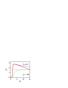
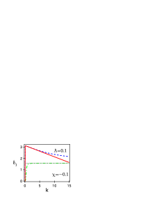
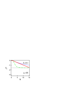
Figure 1: Scattering phase shift for $l=1$ short range potential $\delta_{1}$ with generalized boundary condition given by $\Lambda$ and $\chi$. The solid lines represent the full results, while the dashed line the short range approximation with renormalized strength and generalized effective range. The calculations without the generalized effective range is represented by dashed-dotted line. The resonance found in $\chi_{1}=-25$ and $\chi_{1}=-0.1$ are related to the poles of the scattering matrix, which, according to (34), are given by $k_{pole}=1.5-0.12\textrm{i}$ and $k_{pole}=0.10-0.0005\textrm{i}$, respectively.

In figure 1, the scattering phase shifts $\delta_{1}$ is plotted as a function of the incident momentum $k$. The results of the full solution with direct calculation from the boundary condition (17) are shown in full lines, while the results of the two-parameter shape-independent scattering formula (33) are shown with dashed lines. They are in excellent agreement up to $k\Lambda\approx 0.5$ as expected in the preceding analysis. The important point to note is the accuracy with which the resonance is described. The dashed-dotted lines are the results of “wrong” zero-range forrmula using only the first term of (33), which is plotted just to show the critical importance of the $k^{2}$ term. Calculations with higher $l$ than one also yield very similar results showing the power of shape-independent scattering formula (33). Our formula should be useful in the analysis of nuclear and atomic scattering experiments.

4 Conclusion

It has been established for long time that the quantum zero-range interaction in dimension three is trivial except in the spherical channel $l=0$. However, the convincing physical reasoning is given in this work for the first time. In the process of the analysis, we have found a simple general formula for the short-range scattering for any angular momentum $l$. Through the numerics, we have established that this formula indeed is a meaningful generalization of well known result of $l=0$, and that is in spite of the fact that it looses the meaning entirely in strict $\Lambda\to 0$ limit because of the divergence.

The triviality of three-dimensional zero-range interaction is in stark contrast against the richness of one-dimensional zero-range interaction, for which there are infinite variety described by four-parameter family. A similar analysis to this work for the two-dimensional short-range interaction is to be done, if any necessity arises for the examination of quantum two-dimensional scattering.

References

- [1] S. Albeverio, F. Gesztesy, R. H gh-Krohn, and H. Holden, “Solvable Models in Quantum Mechanics”, 2nd Ed. with appendix by P. Exner, (AMS Chelsea, Rhode Island, 2005).
- [2] V. Kostrykin, R. Schrader: Kirchhoff’s rule for quantum wires, J. Phys. A: Math. Gen. 32 (1999), 595–630.
- [3] T. Cheon, P. Exner and O. Turek, Approximation of a general singular vertex coupling in quantum graphs, Ann. Phys. (NY) 325 (2010) 548–578.
- [4] R. Jackiw,“Diverse Topics in Theoretical and Mathematical Physic”, (World Scientific, Singapore, 1995).
- [5] M. V. Berry, Hermitian boundary conditions at a Dirichlet singularity: the Marletta-Rozenblum model, J. Phys. A: Math. Theor. 42 165208 (13p).
- [6] R. G. Newton, “Scattering theory of waves and particles”, (McGraw-Hill, New York, 1966).