Iterative solution of a Dirac equation with inverse Hamiltonian method

Abstract

We solve a singe-particle Dirac equation with Woods-Saxon potentials using an iterative method in the coordinate space representation. By maximizing the expectation value of the inverse of the Dirac Hamiltonian, this method avoids the variational collapse, in which an iterative solution dives into the Dirac sea. We demonstrate that this method works efficiently, reproducing the exact solutions of the Dirac equation.

The imaginary time method has been successfully employed in non-relativistic self-consistent mean-field calculations DFKW80 ; ev8 . The idea of this method is that a function $e^{-H\tau/\hbar}|\psi_{0}\rangle$ converges to the ground state wave function of a Hamiltonian $H$ as $\tau\to\infty$ for any trial wave function $|\psi_{0}\rangle$ as long as it is not an eigenstate of $H$. One can then iteratively seek for the eigenfunctions of $H$ in the coordinate space starting from an arbitrary wave function $|\psi_{0}\rangle$. This method is suitable particularly for self-consistent mean-field calculations in a three-dimensional coordinate space, with which an arbitrary shape of nuclei can be efficiently described BFH85 .

A naiive extension of this method to a relativistic equation, however, meets a serious problem. That is, a Hamiltonian $H$ has both the Fermi and Dirac seas (see Fig. 1) and an iterative solution inevitably ends up with a wave function in the Dirac sea even if the starting wave function $|\psi_{0}\rangle$ is in the Fermi sea. This problem was recently pointed out in Ref. ZLM10 in the nuclear physics context, although the problem had been well known in quantum chemistry under the name of variational collapse G82 ; LM82 ; SH84 ; HK94 ; PM95 ; FFC97 ; DESV00 ; K07 . In Ref. ZLM10 , the problem was avoided by applying the imaginary time method to the Schrödinger-equivalent form of the Dirac equation. The same method was used also in Ref. GM07 . Moreover, damped relaxation techniques were employed in Ref. BSUR89 for an iterative solution of a Dirac equation.

In this paper, we propose a yet another method for iterative solution of a Dirac equation, which can be directly applied to the coordinate space representation of a relativistic wave function. The method is based on the idea of Hill and Krauthauser HK94 to maximize the expectation value of the inverse Hamiltonian. This method solves the Dirac equation as it is and thus both the upper and lower components of a wave function are automatically obtained. Also, in this method, states in the Dirac sea can be obtained within the same scheme by inverting the direction of “time” evolution, while the method in Refs. ZLM10 ; GM07 requires two different equations for the Fermi and Dirac seas. Thus, our method can be regarded complementary to the method in Refs. ZLM10 ; GM07 .

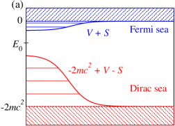
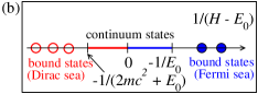
Figure 1: (Color online) (a) A schematic spectrum of a Dirac Hamiltonian $H$. $V(r)$ and $S(r)$ are vector and scalar potentials, respectively. $E_{0}$ is an arbitrary constant located between the lowest energy state in the Fermi sea and the highest energy state in the Dirac sea. The hatched regions indicate the continuum spectra. (b) A spectrum of $1/(H-E_{0})$ corresponding to Fig. 1(a). The filled circles indicate the bound states in the Fermi sea, while the open circles indicate the bound states in the Dirac sea. The continuum region is denoted by the thick solid line.

In our method, the ground state wave function $|\Psi\rangle$ of a Dirac Hamiltonian $H$ is obtained by using the relation

$$|\Psi\rangle\propto\lim_{T\to\infty}e^{\frac{T}{H-E_{0}}}|\psi_{0}\rangle,$$ (1)

where $E_{0}$ is a constant between the lowest eigenvalue in the Fermi sea and the highest eigenvalue in the Dirac sea. In order to illustrate how this method works, Fig. 1 shows a spectrum of $H$ (Fig. 1 (a)) and that of $1/(H-E_{0})$ (Fig. 1 (b)) HK94 . In the spectrum of $1/(H-E_{0})$ shown in Fig. 1(b), the states in the Fermi sea appear in the positive region while those in the Dirac sea in the negative region. Therefore, as $T\to\infty$ in Eq. (1), all the states in the Dirac sea are damped out. Moreover, the lowest energy state in the Fermi sea corresponds to the highest point in Fig. 1(b), and only this state survives in Eq. (1) as $T\to\infty$.

In practice, Eq. (1) is solved iteratively. That is, from the wave function at $T\equiv n\Delta T$, $|\Psi^{n}\rangle$, the wave function is evolved with a small interval $\Delta T$ as

$$|\Psi^{n+1}\rangle\sim\left(1+\frac{\Delta T}{H-E_{0}}\right)\,|\Psi^{n}\rangle.$$ (2)

The inverse of the Hamiltonian is in a familiar form in non-relativistic time-dependent Hartree-Fock (TDHF) calculations KDM77 ; KM90 (see also Ref. BGS83 for a similar technique in relativistic TDHF calculations), and one can evaluate the inverse similarly to Refs. KDM77 ; KM90 ; BGS83 using the Gauss elimination method. We demonstrate it here for spherical potentials. The relativistic wave function then takes the formS67 ; G97 ,

$$\Psi(\mbox{\boldmath$r$})=\frac{1}{r}\left(\begin{array}[]{c}G(r){\cal Y}_{jlm}(\hat{\mbox{\boldmath$r$}})\\ iF(r){\cal Y}_{j\tilde{l}m}(\hat{\mbox{\boldmath$r$}})\end{array}\right),$$ (3)

where $\tilde{l}=2j-l=j\pm 1/2$ for $l=j\mp 1/2$, and

$${\cal Y}_{jlm}(\hat{\mbox{\boldmath$r$}})=\sum_{m_{l},m_{s}}\left.\left\langle l\,m_{l}\,\frac{1}{2}\,m_{s}\right|jm\right\rangle Y_{lm_{l}}(\hat{\mbox{\boldmath$r$}})\chi_{m_{s}},$$ (4)

is the spin-angular wave function, $Y_{lm_{l}}$ and $\chi_{m_{s}}$ being the spherical harmonics and the spin wave function, respectively. The Dirac equation with a spherical vector potential $V(r)$ and a scalar potential $S(r)$ then readsS67 ; G97 ,

$$\left(\begin{array}[]{cc}U&\hbar c\left(-\frac{d}{dr}+\frac{\kappa}{r}\right)\\ \hbar c\left(\frac{d}{dr}+\frac{\kappa}{r}\right)&W-2mc^{2}\end{array}\right)\left(\begin{array}[]{c}G\\ F\end{array}\right)=E\left(\begin{array}[]{c}G\\ F\end{array}\right),$$ (5)

where $\kappa=\mp(j+1/2)$ for $j=l\pm 1/2$, $U(r)=V(r)+S(r)$, and $W(r)=V(r)-S(r)$. It is easy to show that $G$ and $F$ are proportional to $r^{l+1}$ and $r^{\tilde{l}+1}$, respectively, around the origin, $r\sim 0$. Notice that $|\Psi^{n+1}\rangle$ satisfies $(H-E_{0})|\Psi^{n+1}\rangle=(H-E_{0}+\Delta T)|\Psi^{n}\rangle$ (see Eq. (2)). This implies that $G$ and $F$ at $T+\Delta T$ satisfy

$$\left(\begin{array}[]{cc}U-E_{0}&\hbar c\left(-\frac{d}{dr}+\frac{\kappa}{r}\right)\\ \hbar c\left(\frac{d}{dr}+\frac{\kappa}{r}\right)&W-2mc^{2}-E_{0}\end{array}\right)\left(\begin{array}[]{c}G^{n+1}(r)\\ F^{n+1}(r)\end{array}\right)$$ (10)

$$\hskip 142.26378pt=\left(\begin{array}[]{c}\widetilde{G}^{n}(r)\\ \widetilde{F}^{n}(r)\end{array}\right),$$ (13)

where $\widetilde{G}$ and $\widetilde{F}$ are defined as

$$\left(\begin{array}[]{c}\widetilde{G}^{n}(r)\\ \widetilde{F}^{n}(r)\end{array}\right)$$ (16)

$$\equiv\left(\begin{array}[]{cc}U-E_{0}+\Delta T&\hbar c\left(-\frac{d}{dr}+\frac{\kappa}{r}\right)\\ \hbar c\left(\frac{d}{dr}+\frac{\kappa}{r}\right)&W-2mc^{2}-E_{0}+\Delta T\end{array}\right)\left(\begin{array}[]{c}G^{n}(r)\\ F^{n}(r)\end{array}\right).$$ (21)

We solve these equations by discretizing the radial coordinate with a spacing of $\Delta r$ and imposing the box boundary condition, that is, the wave functions vanish at the edge of the box. Denoting the wave functions at $r_{k}\equiv k\Delta r$ as $G_{k}$ and $F_{k}$, and using the three-point formula for the first derivative, $\psi^{\prime}_{k}\sim(\psi_{k+1}-\psi_{k-1})/2\Delta r$, Eq. (13) reads

$$\mbox{\boldmath$\phi$}_{k+1}+\mbox{\boldmath$A$}_{k}\mbox{\boldmath$\phi$}_{k}-\mbox{\boldmath$\phi$}_{k-1}=\mbox{\boldmath$b$}_{k},$$ (23)

with

$$\mbox{\boldmath$\phi$}_{k}\equiv\left(\begin{array}[]{c}G_{k}^{n+1}\\ F_{k}^{n+1}\end{array}\right),~{}~{}~{}~{}~{}~{}\mbox{\boldmath$b$}_{k}\equiv\frac{2\Delta r}{\hbar c}\left(\begin{array}[]{c}\widetilde{F}_{k}^{n}\\ -\widetilde{G}_{k}^{n}\end{array}\right).$$ (24)

Here, $\mbox{\boldmath$A$}_{k}$ is a 2$\times$2 matrix defined by

$$\mbox{\boldmath$A$}_{k}\equiv\left(\begin{array}[]{cc}\frac{2\Delta r}{r_{k}}\kappa&\frac{2\Delta r}{\hbar c}(W_{k}-E_{0}-2mc^{2})\\ -\frac{2\Delta r}{\hbar c}(U_{k}-E_{0})&-\frac{2\Delta r}{r_{k}}\kappa\end{array}\right).$$ (25)

We assume

$$\mbox{\boldmath$\phi$}_{k+1}=\mbox{\boldmath$\alpha$}_{k}\mbox{\boldmath$\phi$}_{k}+\mbox{\boldmath$\beta$}_{k},$$ (26)

where $\mbox{\boldmath$\alpha$}_{k}$ is a 2$\times$2 matrix and $\mbox{\boldmath$\beta$}_{k}$ is a two-component vector. Substituting this to Eq. (23), one finds

$$\mbox{\boldmath$\alpha$}_{k-1} = (\mbox{\boldmath$A$}_{k}+\mbox{\boldmath$\alpha$}_{k})^{-1},$$ (27)

$$\mbox{\boldmath$\beta$}_{k-1} = (\mbox{\boldmath$A$}_{k}+\mbox{\boldmath$\alpha$}_{k})^{-1}(\mbox{\boldmath$b$}_{k}-\mbox{\boldmath$\beta$}_{k}).$$ (28)

These equations can be solved inwards from $r_{N-1}$ with $\mbox{\boldmath$\alpha$}_{N-1}=\mbox{\boldmath$\beta$}_{N-1}=0$, which ensures that the wave functions vanish at $R_{\rm max}=r_{N}$. Once $\mbox{\boldmath$\alpha$}_{k}$ and $\mbox{\boldmath$\beta$}_{k}$ are so obtained, the wave functions $\mbox{\boldmath$\phi$}_{k}$ can be constructed with Eq. (26) outwards from $\mbox{\boldmath$\phi$}_{k=0}=0$.

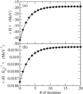
Figure 2: The expectation value of the Hamiltonian $H$ (Fig. 2(a)) and that of the inverse of the Hamiltonian, $1/(H-E_{0})$, (Fig. 2(b)) at each iteration for the neutron 1p_1/2 state in ¹⁶O. $E_{0}$ is set to be the depth of the Woods-Saxon potential $U(r)=V(r)+S(r)$, and the step $\Delta T$ is taken to be 10 MeV.

Let us now numerically investigate the performance of the inverse Hamiltonian method. To this end, we use spherical Woods-Saxon potentials for $U(r)$ and $W(r)$ which correspond to ¹⁶O. The parameters of the Woods-Saxon potentials are taken from Ref. KR91 . Figure 2 shows the convergence feature for the neutron 1p_1/2 state ($\kappa=1$), where the quantum numbers refer to the upper component of the wave function. The coordinate space is discretized up to $R_{\rm max}$=15 fm with $\Delta r=0.1$ fm. The energy shift $E_{0}$ is taken to be the depth of the potential $U(r)$, that is, $E_{0}=-71.28$ MeV, and the size of step $\Delta T$ is taken to be 10 MeV. For the initial wave functions, we take $F(r)=0$ and $G(r)$ to be the non-relativistic 1p_1/2 wave function of a Woods-Saxon potential with $V_{0}=-51$ MeV, $R_{0}=1.27\times 16^{1/3}$ fm, and $a$=0.67 fm ZMR03 . Fig. 2(a) indicates that the energy of the 1p_1/2 state is quickly converged as the number of iteration increases. The converged value is $E=-18.974$ MeV, that is almost identical to the exact value, $E=-18.976$ MeV. Fig. 2(b) also shows that the expectation value of the inverse of the Hamiltonian,

$$\langle(H-E_{0})^{-1}\rangle=\frac{1}{\Delta T}\cdot\left\langle\Psi^{n}\left|\left(1+\frac{\Delta T}{H-E_{0}}\right)\,\right|\Psi^{n}\right\rangle-\frac{1}{\Delta T},$$ (29)

monotonically increases to the converged value, although it may not be the case for $\langle H\rangle$.

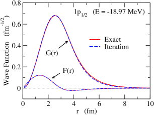
Figure 3: (Color online) Comparison of the wave function for the neutron 1p_1/2 state in ¹⁶O obtained with the inverse Hamiltonian method (the dashed lines) to the exact solutions (the solid lines).

Figure 3 shows the wave functions for the 1p_1/2 state. The solid lines show the exact solution of the Dirac equation obtained with the Runge-Kutta method, while the dashed lines show the wave function obtained with the inverse Hamiltonian method. One can clearly see that the iterative method well reproduces the exact wave function.

We have checked that the performance of the inverse Hamiltonian method is good also for other states with different quantum numbers as well, although the accuracy seems to be somewhat improved if the energy shift $E_{0}$ can be chosen as close as possible to the exact value. Evidently, the inverse Hamiltonian method provides an efficient method to solve a Dirac equation iteratively.

Before we close this paper, we would like to point out that the states in the Dirac sea can be also obtained within the same scheme by changing $\Delta T$ by $-\Delta T$ in Eq. (2). This is so because the highest energy state in the Dirac sea corresponds to the minimum of $1/(H-E_{0})$ (see Fig. 1(b)). We have obtained the bound states in the Dirac sea in this way for ¹⁶O, and have confirmed that the exact wave functions are well reproduced.

In summary, we have proposed a new scheme to iteratively solve a Dirac equation. The idea of the new scheme is to maximize the inverse of a shifted Hamiltonian, $1/(H-E_{0})$, and thus we call it the inverse Hamiltonian method. By choosing $E_{0}$ to be between the highest energy in the Dirac sea and the lowest energy in the Fermi sea, the expectation value of $1/(H-E_{0})$ monotonically converges to the exact value, $1/(E-E_{0})$. The upper and the lower components of a wave function can be simultaneously obtained with this method in the coordinate space representation. We have applied this method to neutron states in ¹⁶O using spherical Woods-Saxon potentials. We have shown that the inverse Hamiltonian method efficiently reproduces the exact energies and wave functions for the states both in the Fermi and Dirac seas. In this paper, we have assumed spherical symmetry for nuclear potentials. It will be an interesting future work to apply this method to self-consistent relativistic mean-field calculations in three-dimensional space.

This work was supported by the Grant-in-Aid for Scientific Research (C), Contract No. 22540262 from the Japan Society for the Promotion of Science.

References

- (1) K.T.R. Davies, H. Flocard, S. Krieger, and M.S. Weiss, Nucl. Phys. A342, 111 (1980).
- (2) P. Bonche, H. Flocard, and P.H. Heenen, Compt. Phys. Comm. 171, 49 (2005).
- (3) P. Bonche, H. Flocard, P.H. Heenen, S.J. Krieger, and M.S. Weiss, Nucl. Phys. A443, 39 (1985).
- (4) Y. Zhang, H. Liang, and J. Meng, Int. J. of Mod. Phys. E19, 55 (2010); arXiv:0905.2505 [nucl-th].
- (5) I.P. Grant, Phys. Rev. A25, 1230 (1982).
- (6) Y.S. Lee and A.D. McLean, J. Chem. Phys. 76, 735 (1982).
- (7) R.E. Stanton and S. Havriliak, J. Chem. Phys. 81, 1910 (1984).
- (8) R.N. Hill and C. Krauthauser, Phys. Rev. Lett. 72, 2151 (1994).
- (9) F.A. Parpia and A.K. Mohanty, Phys. Rev. A52, 962 (1995).
- (10) P. Falsaperla, G. Fonte, and J.Z. Chen, Phys. Rev. A56, 1240 (1997).
- (11) J. Dolbeault, M.J. Esteban, E. Sére, M. Vanbreugel, Phys. Rev. Lett. 85, 4020 (2000).
- (12) W. Kutzelnigg, J. Chem. Phys. 126, 201103 (2007).
- (13) P. Gögelein and H. Müther, Phys. Rev. C76, 024312 (2007).
- (14) C. Bottcher, M.R. Strayer, A.S. Umar, and P.-G. Reinhard, Phys. Rev. A40, 4182 (1989).
- (15) S.E. Koonin, K.T.R. Davies, V. Maruhn-Rezwani, H. Feldmeier, S.J. Krieger, and J.W. Negele, Phys. Rev. C15, 1359 (1977).
- (16) S.E. Koonin and D.C. Meredith, Computational Physics (Addison-Wesley, Reading, MA, 1990).
- (17) U. Becker, N. Grün, and W. Scheid, J. of Phys. B16, 1967 (1983).
- (18) J.J. Sakurai, Advanced Quantum Mechanics (Addison-Wesley, Red City, CA, 1967).
- (19) W. Greiner, Relativistic Quantum Mechanics (Springer-Verlag, Berlin, 1997).
- (20) W. Koepf and P. Ring, Z. Phys. A339, 81 (1991).
- (21) S.-G. Zhou, J. Meng, and P. Ring, Phys. Rev. C68, 034323 (2003).