Fluctuation Dynamo and Turbulent Induction at Small Prandtl Number

Abstract

We study the Lagrangian mechanism of the fluctuation dynamo at zero Prandtl number and infinite magnetic Reynolds number, in the Kazantsev-Kraichnan model of white-noise advection. With a rough velocity field corresponding to a turbulent inertial-range, flux-freezing holds only in a stochastic sense. We show that field-lines arriving to the same point which were initially separated by many resistive lengths are important to the dynamo. Magnetic vectors of the seed field that point parallel to the initial separation vector arrive anti-correlated and produce an “anti-dynamo” effect. We also study the problem of “magnetic induction” of a spatially uniform seed field. We find no essential distinction between this process and fluctuation dynamo, both producing the same growth-rates and small-scale magnetic correlations. In the regime of very rough velocity fields where fluctuation dynamo fails, we obtain the induced magnetic energy spectra. We use these results to evaluate theories proposed for magnetic spectra in laboratory experiments of turbulent induction.

I Introduction

Hannes Alfvén introduced the notion of magnetic flux conservation in ideal magnetohydrodynamics Alfvén (1942). This property of “flux-freezing” involves an implicit assumption, however, that plasma fluid velocities remain smooth in the limit of vanishing resistivity. This assumption need not be valid if the viscosity vanishes together with the resistivity, at a fixed or a decreasing magnetic Prandtl number. At the implied high Reynolds numbers, smooth laminar plasma flows will be unstable to the development of turbulence. We have argued previously that magnetic flux-conservation in its usual sense cannot hold at any small resistivities, no matter how tiny, in a turbulent plasma with a Kolmogorov-like energy spectrum Eyink and Aluie (2006). Neither is flux-freezing completely broken but, instead, it becomes intrinsically stochastic due to the roughness of the advecting velocity field Eyink (2007, 2009). Infinitely-many magnetic field lines are carried to each point—even in the limit of very high conductivity—which must be averaged to obtain the resultant magnetic field at that point.

The previous ideas are theoretical predictions for turbulent flows of astrophysical and laboratory plasmas. However, they are exact properties of at least one soluble problem of turbulent advection, the Kazantsev-Kraichnan (KK) model of kinematic magnetic dynamo. See Kazantsev (1968); Kraichnan and Nagarajan (1967); Kraichnan (1968) and many following papers Ruzmaĭkin and Sokolov (1981); Novikov et al. (1983); Vergassola (1996); Rogachevskii and Kleeorin (1997); Vincenzi (2002); Boldyrev and Cattaneo (2004); Boldyrev et al. (2005); Celani et al. (2006); Arponen and Horvai (2007). In that model the physical turbulent velocity field is replaced by a Gaussian random field that is white-noise in time and rough (Hölder continuous) in space. It is rigorously established for this model that Lagrangian particle trajectories are “spontaneously stochastic” in the limit of infinite Reynolds numbers, with an infinite ensemble of trajectories for a given advecting velocity field and a given initial particle position Bernard et al. (1998); Gawȩdzki and Vergassola (2000); Chaves et al. (2003); E and Vanden-Eijnden (2000, 2001); Jan and Raimond (2002, 2004); Kupiainen (2003). This remarkablebreakdown of Laplacian determinism is a consequence of the properties of two-particle Richardson diffusion Richardson (1926), which are also expected to hold for real fluid turbulence.

The stochastic nature of flux-freezing must play an essential role in the turbulent magnetic dynamo at high kinetic Reynolds numbers, either for fixed or for vanishing magnetic Prandtl numbers. The zero Prandtl-number fluctuation dynamo was studied in an earlier work of Eyink and Neto Eyink and Neto (2010), hereafter referred to as I, primarily for the KK model. This model undergoes a remarkable transition as the scaling exponent $\xi$ of the velocity structure function is decreased, with dynamo effect disappearing for $\xi<1$ in space dimension three. This seems rather counterintuitive, because velocity-gradients and line-stretching rates in the model increase as $\xi$ is lowered, which should favor dynamo action. Paper I showed that the stochasticity of flux-freezing is fundamental to understand this transition. Although magnetic line-stretching rates indeed increase for decreasing $\xi,$ the resultant magnetic field at a point is the average of infinitely-many field lines advected to that point from a large spatial volume. As shown in I, the correlations between independent line-vectors are small for $\xi<1,$ when the velocity field is too rough, and the net magnetic field decays despite the rapid growth in strength of individual field lines.

The contribution of flux-line stochasticity to turbulent dynamo action for $\xi>1$ was not fully explicated in I, however. Infinitely-many field lines are advected to each point from a large spatial volume, e.g. with diameter of order the velocity integral length $L$ in one turbulent turnover time $L/u_{rms}.$ But all of these field lines are unlikely to make an equal contribution to dynamo action. In particular, field vectors that arrive to the same point from very distant initial locations must be poorly correlated and give small (or negative) dynamo effect. It is not hard to guess that dynamo action in the limit of high-Reynolds number $Lu_{rms}/\nu\gg 1$ and low Prandtl number $\nu/\eta\ll 1$ must arise mainly from vectors with initial separation distances $r$ of order $\sim\ell_{\eta},$ the resistive length. Indeed, this is the only available length-scale in that limit, on dimensional grounds. The exact contribution to fluctuation dynamo from vectors with initial separation $r$ remains unknown, however, even in the KK model. One of the main purposes of this paper to provide a quantitative answer to this problem.

Another important issue left unresolved in I was the outcome of a spatially-uniform initial magnetic field in the dynamo regime of the KK model for $\xi>1.$ Can such a magnetic field provide the seed for a small-scale fluctuation-dynamo? This question is very closely connected with the proper formulation of the concept of “magnetic induction” . This process is usually defined as the creation of small-scale magnetic fluctuations by the turbulent “shredding” of a non-zero mean magnetic field and has been invoked to explain small-scale magnetic fluctuations in liquid metal experiments Odier et al. (1998); Bourgoin et al. (2002); Peffley et al. (2000); Spence et al. (2006); Nornberg et al. (2006), in related numerical simulations Bayliss et al. (2007); Schekochihin et al. (2007), and at the solar surface Brandenburg and Subramanian (2005); Schüssler and Vögler (2008). It is frequently suggested that this process is distinct from fluctuation dynamo. For example, Schekochihin et al. wrote: “Given a multiscale observed or simulated magnetic field, one does not generally have enough information (or understanding), to tell whether it has originated from the fluctuation dynamo, from the mean-field dynamo plus the turbulent induction or from some combination of the two.” Schekochihin et al. (2007) However, if a mean magnetic field can provide a seed for fluctuation dynamo, is there really any meaningful physical distinction between the two mechanisms? Or if magnetic induction is defined instead as a process that occurs only in the absence of fluctuation dynamo, as it sometimes is, then how can one regard the two processes as acting in “combination”? Clearly there is some conceptual confusion in the literature about the proper definition of magnetic induction. We shall use our exact results in the KK model to discuss these issues and, also, to evaluate some the proposed theories of the induced magnetic spectrum.

The contents of this paper are as follows. In section II we provide more detailed background to our work and a more formal statement of the problems to be studied. In section III we study the Lagrangian mechanism of the fluctuation dynamo at zero Prandtl number and the quantitative role of stochastic flux-freezing. A first subsection III.1 presents exact mathematical analysis and the second subsection III.2 gives numerical results. The next section IV discusses the problem of magnetic induction using our analytical results for the KK model. We draw our final conclusions in section V. Appendices A and B present some technical material.

II Background and Problem Statement

We begin this section with a summary of the key results of Paper I. A “dynamo order-parameter” was introduced there with purely geometric significance. Let ${\bf x}({\bf a},t)$ be a stochastic Lagrangian trajectory, satisfying

$$d{\bf x}={\bf u}({\bf x},t)dt+\sqrt{2\eta}\,d{\bf W}(t),\,\,\,\,\,\,{\bf x}(t_{0})={\bf a}.$$ (1)

We shall assume in this section that the advecting velocity field is incompressible, $\hbox{\boldmath$\nabla$}\hbox{\boldmath$\cdot$}{\bf u}=0,$ as in I. ${\bf W}(t)$ in (1) is a vector Brownian motion and $\eta$ is the resistivity (or, in fact, the magnetic diffusivity). Let $\hbox{\boldmath$\ell$}_{k}({\bf a},t)$ be a passive vector starting as a unit vector $\hat{{\bf e}}_{k}$ at space point ${\bf a}$ and time $t_{0}$ and subsequently transported along ${\bf x}({\bf a},t),$ stretched and rotated by the velocity-gradient. That is,

$$\hbox{\boldmath$\ell$}_{k}({\bf a},t)=\hat{{\bf e}}_{k}\hbox{\boldmath$\cdot$}\hbox{\boldmath$\nabla$}_{a}{\bf x}({\bf a},t).$$ (2)

Then I introduced the quantity

$$\mathcal{R}_{k\ell}({\bf r},t)=\langle\overline{\hbox{\boldmath$\ell$}_{k}({\bf a},t)\hbox{\boldmath$\cdot$}\hbox{\boldmath$\ell$}_{\ell}^{\prime}({\bf a}^{\prime},t)\delta^{3}({\bf x}({\bf a},t)-{\bf x}^{\prime}({\bf a}^{\prime},t))}\rangle,$$ (3)

with ${\bf r}={\bf a}-{\bf a}^{\prime},$ where $\langle\cdot\rangle$ denotes average over the turbulent velocity realizations, $\overline{(\cdot)}$ denotes average over the random Brownian motions and $\prime$ indicates a second, independent realization of the latter. This quantity measures not only the magnitude but also the angular correlation of independent line-vectors that start as unit vectors $\hbox{\boldmath$\ell$}_{k}({\bf a},t_{0})={\bf e}_{k},\,\hbox{\boldmath$\ell$}_{\ell}^{\prime}({\bf a}^{\prime},t_{0})={\bf e}_{\ell}$ at points ${\bf a},{\bf a}^{\prime}$ separated by displacement ${\bf r},$ which end at the same point at time $t.$

Now let ${\bf B}$ be a magnetic field kinematically transported by the random velocity field ${\bf u}$ and diffused by resistivity $\eta$:

$$\partial_{t}{\bf B}+({\bf u}\hbox{\boldmath$\cdot$}\hbox{\boldmath$\nabla$}){\bf B}=({\bf B}\hbox{\boldmath$\cdot$}\hbox{\boldmath$\nabla$}){\bf u}+\eta\triangle{\bf B},\,\,\,\,\,\,{\bf B}(t_{0})={\bf B}_{(0)}.$$ (4)

As shown in I, the mean energy in this magnetic field can be expressed as

$$\langle B^{2}(t)\rangle=\int d^{3}r\,\mathcal{R}_{k\ell}({\bf r},t)\langle B^{k}_{(0)}({\bf r})B^{\ell}_{(0)}(\hbox{\boldmath$0$})\rangle.$$ (5)

It has been assumed in deriving (5) that initial conditions on the magnetic field are statistically independent of the velocity and that both quantities are statistically homogeneous (space translation-invariant). This formula makes clear the close relation of dynamo action to the line-correlation (3), which grows exponentially rapidly precisely in the dynamo regime.

This connection was verified in I by an exact calculation of the line-correlation (3) in the soluble Kazantsev-Kraichnan (KK) model of turbulent dynamo Kazantsev (1968); Kraichnan and Nagarajan (1967); Kraichnan (1968); Vergassola (1996); Rogachevskii and Kleeorin (1997); Vincenzi (2002); Boldyrev and Cattaneo (2004); Boldyrev et al. (2005); Celani et al. (2006); Arponen and Horvai (2007). This model replaces the true turbulent velocity by a Gaussian random field which is white-noise in time:

$$\langle u^{i}({\bf x},t)u^{j}({\bf x}^{\prime},t^{\prime})\rangle=\kappa^{ij}({\bf r})\delta(t-t^{\prime})$$ (6)

with ${\bf r}={\bf x}-{\bf x}^{\prime}.$ In this model, the magnetic correlation function

$$\mathcal{C}^{ij}({\bf r},t)=\langle B^{i}({\bf r},t)B^{j}(\hbox{\boldmath$0$},t)\rangle$$ (7)

evolves according to a closed, linear equation

$$\partial_{t}\mathcal{C}^{ij}=\mathcal{M}^{ij}_{k\ell}\mathcal{C}^{k\ell},$$ (8)

where $\mathcal{M}$ is a singular diffusion operator. If $\kappa^{ij}({\bf r})\sim r^{\xi}$ for small $r,$ with rugosity exponent $0<\xi<2,$ then the velocity realizations are rough in space and provide a qualitatively good model of turbulent advection. It was shown in I that $\mathcal{R}_{k\ell}({\bf r},t)$ in the KK model is the solution of the adjoint equation

$$\partial_{t}\mathcal{R}_{k\ell}=\mathcal{M}_{k\ell}^{ij\,*}\mathcal{R}_{ij}$$ (9)

with initial condition $\mathcal{R}_{k\ell}({\bf r},t)=\delta_{k\ell}\delta^{3}({\bf r}).$ This fact was exploited to show that $\mathcal{R}_{k\ell}({\bf r},t)$ in the KK model at zero magnetic Prandtl number, as expected, grows exponentially in the dynamo regime ($\xi>1$) but has only power-law time-dependence in the non-dynamo regime ($\xi<1$).

The study in I left open, however, several important questions. First, what range of $r=|{\bf r}|$ substantially contributes to the correlation $\mathcal{R}$ and to the space-integral in (5)? It is known in the KK model that magnetic field lines arrive to a point from a spatial region with radius $L(t)\sim(t-t_{0})^{1/(2-\xi)},$ in the root-mean-square sense. This is also expected for kinematic dynamo in a real turbulent fluid, where $\xi\doteq 4/3$ and $L(t)\sim(t-t_{0})^{3/2}$ corresponds to turbulent Richardson diffusion of the field lines. However, not all of the field lines in this large volume should be expected to contribute equally to dynamo action. Field vectors starting from points separated by distances $r$ much larger than the resistive length-scale may arrive at the same point with small angular correlations and thus contribute little to net magnetic field growth. It follows from the analysis of I for the KK model in its dynamo regime that, for times $t$ long compared to the resistive time-scale,

$$\mathcal{R}_{k\ell}({\bf r},t)\sim e^{-\lambda t}\mathcal{\widetilde{G}}_{k\ell}({\bf r}),\,\,\,\,\,\,\,\,\,\,(\lambda<0)$$ (10)

where $-\lambda$ is the largest (positive) eigenvalue of $\mathcal{M}^{*}$ and $\mathcal{\widetilde{G}}$ is the corresponding (right) eigenmode. Thus, questions about the spatial structure of $\mathcal{R}$ reduce, in the exponential growth regime at sufficiently long times, to the corresponding questions about the right eigenmode $\mathcal{\widetilde{G}}$ of $\mathcal{M}^{*}$ (or, equivalently, left eigenmode of $\mathcal{M}$). It is one of the goals of the present work to calculate this eigenmode and thereby determine the degree of correlation of line-vectors arriving from various initial separations.

A second important issue left unresolved in I was the response of a spatially uniform initial magnetic field to turbulent advection and stretching. In the case of a uniform initial field, formula (5) simplifies to

$$\langle B^{2}(t)\rangle=\mathcal{R}_{k\ell}(t)\langle B^{k}_{(0)}B^{\ell}_{(0)}\rangle,$$ (11)

with

$$\mathcal{R}_{k\ell}(t)\equiv\int d^{3}r\,\mathcal{R}_{k\ell}({\bf r},t)=\langle\hbox{\boldmath$\ell$}_{k}(t)\hbox{\boldmath$\cdot$}\hbox{\boldmath$\ell$}_{\ell}^{\prime}(t)\rangle_{0}.$$ (12)

The quantity (12) measures the correlation of two independent line-vectors that arrive at the same point, regardless of their initial separation. The result (10) does not imply exponential growth of this integrated correlation, however, unless one can show that

$$\int d^{3}r\,\mathcal{\widetilde{G}}_{k\ell}({\bf r})\neq 0.$$ (13)

Below we shall demonstrate this fact.

This result is closely connected with another important physical problem, the creation of small-scale magnetic fluctuations by turbulent “magnetic induction” of a non-zero mean-field Odier et al. (1998); Bourgoin et al. (2002); Peffley et al. (2000); Spence et al. (2006); Nornberg et al. (2006); Bayliss et al. (2007); Schekochihin et al. (2007). Indeed, the formula (11) applies directly to this situation, which corresponds to the special case $\langle B^{k}_{(0)}B^{\ell}_{(0)}\rangle=\langle B^{k}_{(0)}\rangle\langle B^{\ell}_{(0)}\rangle.$ This observation already makes clear that there is no essential physical distinction between “fluctuation dynamo” and “magnetic induction”, which simply correspond to different choices of initial magnetic field (random vs. deterministic). Other definitions of “magnetic induction” are offered in the literature. If the fluctuation dynamo fails to operate for some reason (e.g. if the magnetic Reynolds number is too small), then the term “magnetic induction” is sometimes used for the process by which small-scale fluctuations are generated from the mean magnetic field. If a mean-field dynamo still operates and creates an exponentially growing large-scale magnetic field, then these “parasitic” small-scale fluctuations may be also exponentially increasing. This provides another mechanism to produce exponential growth of small-scale magnetic fields in the absence of a fluctuation dynamo. If instead there is no mean-field dynamo, then such growth of small-scale fluctuations by “magnetic induction” is sub-exponential. We shall discuss below the non-dynamo regime $(\xi<1)$ of the KK model as a simple example of such “magnetic induction” and use it to evaluate some physical theories that have been proposed for the phenomenon.

We mention finally one additional motivation to study the left eigenmodes of $\mathcal{M}.$ As pointed out in I, these have a physical interpretation as correlators of the magnetic vector potential ${\bf A}.$ More precisely, the correlation function defined by

$$\mathcal{G}_{k\ell}({\bf r},t)=\langle A_{k}({\bf r},t)A_{\ell}(\hbox{\boldmath$0$},t)\rangle,$$ (14)

in the KK model satisfies

$$\partial_{t}\mathcal{G}_{k\ell}=\mathcal{M}_{k\ell}^{ij\,*}\mathcal{G}_{ij},$$ (15)

with diffusion operator adjoint to that in eq.(8). The underlying reason for this fact is the conservation of magnetic helicity $H=\int d^{3}r\,{\bf A}\hbox{\boldmath$\cdot$}{\bf B}$ for the ideal induction equation. If the latter is written as

$$\partial_{t}{\bf B}=\mathcal{L}{\bf B},$$ (16)

for a linear operator $\mathcal{L}$ (depending on the velocity ${\bf u}$), then helicity conservation is equivalent to

$$\partial_{t}{\bf A}=-\mathcal{L}^{*}{\bf A},$$ (17)

up to addition of a gradient term. Different operators $\mathcal{L}$ are possible, which coincide in their action on solenoidal magnetic fields ($\hbox{\boldmath$\nabla$}\hbox{\boldmath$\cdot$}{\bf B}=0$), but whose adjoints $\mathcal{L}^{*}$ correspond to different gauge choices for ${\bf A}.$ Equation (17) directly implies (15) in the KK model. The addition of resistivity to eqs. (16), (17) does not change this result, since the additional Laplacian operator is self-adjoint.

III Fluctuation Dynamo

We study in this section the Lagrangian mechanism of the fluctuation dynamo in the KK model for three space-dimensions (3D) and for homogeneous and isotropic statistics of both velocity and magnetic fields. We begin in the first subsection III.1 with exact mathematical analysis of the problem. Most of this discussion applies to a fairly general situation, allowing for compressibility and helicity of the velocity field. We then specialize to the case of an incompressible, non-helical advecting velocity, with a power-law space-correlation corresponding to an infinite-Reynolds-number inertial-range range for the velocity field. In the second subsection III.2 we present numerical results for this latter case and discuss their physical interpretation. The reader who is mostly interested in the final results, and not their detailed derivation, may skip directly to that section of the paper.

III.1 Mathematical Analysis

We discuss two natural choices for the linear operator $\mathcal{L}$ in the ideal induction eq.(16) and the corresponding adjoint operators $\mathcal{L}^{*}$ and gauge choices for the vector potential, successively in the following two subsections.

III.1.1 Gauge I

One choice to write the induction equation is as

$$\partial_{t}{\bf B}=\hbox{\boldmath$\nabla$}\hbox{\boldmath$\times$}({\bf u}\hbox{\boldmath$\times$}{\bf B}-\eta\hbox{\boldmath$\nabla$}\hbox{\boldmath$\times$}{\bf B}).$$ (18)

Note that in the ideal equation with $\eta=0,$ $\mathcal{L}_{\bf u}^{(2)}{\bf B}=-\hbox{\boldmath$\nabla$}\hbox{\boldmath$\times$}({\bf u}\hbox{\boldmath$\times$}{\bf B})$ is the Lie-derivative acting on ${\bf B}$ as a differential 2-form. See Larsson (2003), eq.(2.3) for $\hbox{\boldmath$\nabla$}\hbox{\boldmath$\cdot$}{\bf B}=0.$ Thus, this form of the induction equation is most directly connected with the conservation of magnetic flux through advected 2-dimensional surfaces. The corresponding adjoint equation for the vector potential is

$$\partial_{t}{\bf A} = {\bf u}\hbox{\boldmath$\times$}(\hbox{\boldmath$\nabla$}\hbox{\boldmath$\times$}{\bf A})-\eta\hbox{\boldmath$\nabla$}\hbox{\boldmath$\times$}(\hbox{\boldmath$\nabla$}\hbox{\boldmath$\times$}{\bf A})$$ (19)

$$= -({\bf u}\hbox{\boldmath$\cdot$}\hbox{\boldmath$\nabla$}){\bf A}+(\hbox{\boldmath$\nabla$}{\bf A}){\bf u}$$ (21)

$$\,\,\,\,\,\,\,\,\,\,\,\,\,\,\,\,\,\,\,\,\,\,\,\,\,\,\,\,\,\,\,+\eta[\triangle{\bf A}-\hbox{\boldmath$\nabla$}(\hbox{\boldmath$\nabla$}\hbox{\boldmath$\cdot$}{\bf A})].$$

In the gauge-choice implied by this equation, pure-gauge fields ${\bf A}=\hbox{\boldmath$\nabla$}\lambda$ satisfy $\hbox{\boldmath$\nabla$}(\partial_{t}\lambda)=0$ and are, thus, time-independent up to possible spatially constant terms.

Boldyrev, Cattaneo and Rosner in Boldyrev et al. (2005) developed an elegant formulation of the KK model based on the eq.(18) for the case of homogeneous and isotropic statistics. We review their formulation—hereafter referred to as the BCR formalism—in Appendix A, paying special attention to issues of gauge-invariance. Readers not previously familiar with the work of Boldyrev et al. (2005) may wish to review that appendix before proceeding. One essential observation of BCR is that the evolution operator for magnetic correlations factorizes as ${\cal M}={\cal DJ}.$ More precisely, in the KK model starting from eq.(18)

$$\partial_{t}\mathcal{C}^{ij}=\mathcal{M}^{ij}_{pq}\mathcal{C}^{pq}=\mathcal{D}^{ij,k\ell}\mathcal{J}_{k\ell,pq}\mathcal{C}^{pq}$$ (22)

where

$$\mathcal{D}^{ij,k\ell}=\epsilon^{ikp}\epsilon^{j\ell q}\partial_{p}\partial_{q}$$ (23)

is the non-positive, self-adjoint differential operator which relates the magnetic correlation to the vector-potential correlation and

$$\mathcal{J}_{ij,k\ell}=\epsilon_{ikp}\epsilon_{j\ell q}T^{pq}$$ (24)

is the self-adjoint multiplication operator with $T^{pq}({\bf r})=2\eta\delta^{pq}+\kappa^{pq}(0)-\kappa^{pq}({\bf r}),$ where $\kappa^{pq}({\bf r})$ is the spatial velocity-correlation in eq.(6). Explicitly,

$$\mathcal{M}^{ij}_{pq}\mathcal{C}^{pq} = \partial_{r}\partial_{s}\left(T^{rs}\mathcal{C}^{ij}\right)-\partial_{p}\partial_{s}\left(T^{is}\mathcal{C}^{pj}\right)$$ (26)

$$\,\,\,\,\,-\partial_{r}\partial_{q}\left(T^{rj}\mathcal{C}^{iq}\right)+\partial_{p}\partial_{q}\left(T^{ij}\mathcal{C}^{pq}\right).$$

One may further write equations in the KK model for the joint correlations of magnetic and vector-potentials

$$\Psi^{i\,\,\,\,}_{\,\,\,\,k}({\bf r},t)=\langle B^{i}({\bf r},t)A_{k}(\hbox{\boldmath$0$},t)\rangle,\,\,\Psi_{k\,\,\,\,}^{\,\,\,\,i}({\bf r},t)=\langle A_{k}({\bf r},t)B^{i}(\hbox{\boldmath$0$},t)\rangle$$

using the operator $\mathcal{R}^{i,k}=\epsilon^{ipk}\partial_{p},$ in terms of which the operator $\mathcal{D}$ itself factorizes as $\mathcal{D}^{ij,k\ell}=\mathcal{R}^{i,k}\mathcal{R}^{j,\ell}.$ Then

$$\partial_{t}\Psi^{i\,\,\,\,}_{\,\,\,\,n} = -(\mathcal{R}^{i,m})^{*}\mathcal{J}_{mn,pq}\mathcal{R}^{q,\ell}\Psi^{p\,\,\,\,}_{\,\,\,\,\ell}$$ (27)

$$\partial_{t}\Psi_{m\,\,\,\,}^{\,\,\,\,j} = -(\mathcal{R}^{j,n})^{*}\mathcal{J}_{mn,pq}\mathcal{R}^{p,k}\Psi_{k\,\,\,\,}^{\,\,\,\,q}$$ (28)

Finally, the vector-potential correlation in (14) obeys

$$\partial_{t}\mathcal{G}_{k\ell}=(\mathcal{M}^{*})_{k\ell}^{pq}\mathcal{G}_{pq}=\mathcal{J}_{k\ell,rs}\mathcal{D}^{rs,pq}\mathcal{G}_{pq}$$ (29)

with $\mathcal{M}^{*}=\mathcal{JD}.$ Explicitly,

$$(\mathcal{M}^{*})_{k\ell}^{pq}\mathcal{G}_{pq} = T^{rs}\partial_{r}\partial_{s}\mathcal{G}_{k\ell}-T^{ps}\partial_{k}\partial_{s}\mathcal{G}_{p\ell}$$ (31)

$$\,\,\,\,\,-T^{rq}\partial_{r}\partial_{\ell}\mathcal{G}_{kq}+T^{pq}\partial_{k}\partial_{\ell}\mathcal{G}_{pq}.$$

BCR mainly considered the isotropic sector of the KK model, invariant under proper rotations but not necessarily space reflections. In that case, with $\hat{{\bf r}}={\bf r}/r,$

$$\kappa^{ij}({\bf r})=\kappa_{L}(r)\hat{r}^{i}\hat{r}^{j}+\kappa_{N}(r)(\delta^{ij}-\hat{r}^{i}\hat{r}^{j})+\kappa_{H}(r)\epsilon^{ijk}\hat{r}_{k},$$

where $\kappa_{L},\,\,\kappa_{N},$ and $\kappa_{H}=rg$ are conventional longitudinal, transverse and helical correlation functions, with similar representations of $\mathcal{C},\mathcal{G},$ etc. However, ref.Boldyrev et al. (2005) introduced instead a special basis to expand tensor correlation functions, as $\mathcal{C}^{ij}=\sum_{a=1}^{3}C_{a}\xi^{ij}_{a}$ with

$$\xi^{ij}_{1}={{1}\over{\sqrt{2}r}}(\delta^{ij}-\hat{r}^{i}\hat{r}^{j}),\,\,\,\,\xi^{ij}_{2}={{1}\over{r}}\hat{r}^{i}\hat{r}^{j},\,\,\,\,\xi^{ij}_{3}={{1}\over{\sqrt{2}r}}\epsilon^{ijk}\hat{r}^{k},$$

so that

$$C_{1}=\sqrt{2}rC_{N},\,\,\,\,C_{2}=rC_{L},\,\,\,\,C_{3}=\sqrt{2}rC_{H}.$$

The special feature of this basis is that the Hilbert-space inner-product defined by

$$\langle\mathcal{G,C}\rangle=\int d^{3}r\,\,\mathcal{G}_{ij}({\bf r})\mathcal{C}^{ij}({\bf r})$$

simplifies in the isotropic sector to

$$\langle G,C\rangle=4\pi\int_{0}^{\infty}dr\,[G_{1}C_{1}+G_{2}C_{2}+G_{3}C_{3}].$$

We hereafter use the notation $\mathcal{C,G}$ etc. in the BCR formalism for the isotropic sector to represent the column vectors

$$\mathcal{C}=\left(\begin{array}[]{c}C_{1}\cr C_{2}\cr C_{3}\end{array}\right).$$

In this representation, the operators ${\cal J}$ and ${\cal D}$ take the simple forms

$$\mathcal{J}=\left(\begin{array}[]{ccc}b&a&0\cr a&0&c\cr 0&c&b\end{array}\right),\,\,\,\,\,\mathcal{D}=\left(\begin{array}[]{ccc}\partial_{r}^{2}&-\partial_{r}{{\sqrt{2}}\over{r}}&0\cr{{\sqrt{2}}\over{r}}\partial_{r}&-{{2}\over{r^{2}}}&0\cr 0&0&{{1}\over{r^{2}}}\partial_{r}r^{4}\partial_{r}{{1}\over{r^{2}}}\end{array}\right),$$

with

$$a(r)=\sqrt{2}[2\eta+\kappa_{N}(0)-\kappa_{N}(r)]$$

$$b(r)=2\eta+\kappa_{L}(0)-\kappa_{L}(r)$$

$$c(r)=\sqrt{2}[g(0)-g(r)]r.$$

A crucial observation of BCR is that $\mathcal{D}$ factorizes as $\mathcal{D}=-\mathcal{RR}^{*}$ with

$$\mathcal{R}=\left(\begin{array}[]{ccc}0&\partial_{r}&0\cr 0&{{\sqrt{2}}\over{r}}&0\cr 0&0&-{{1}\over{r^{2}}}\partial_{r}r^{2}\end{array}\right),\,\,\,\,\,\,\mathcal{R}^{*}=\left(\begin{array}[]{ccc}0&0&0\cr-\partial_{r}&{{\sqrt{2}}\over{r}}&0\cr 0&0&r^{2}\partial_{r}{{1}\over{r^{2}}}\end{array}\right).$$

Another important fact is that ${\rm Ran}(\mathcal{R}),$ the range of the operator $\mathcal{R},$ consists of the solenoidal functions $\mathcal{C}^{ij}$ that satisfy $\partial_{i}\mathcal{C}^{ij}=\partial_{j}\mathcal{C}^{ij}=0.$ Thus, all solenoidal solutions of the equation $\partial_{t}\mathcal{C}=\mathcal{MC}=-\mathcal{RR}^{*}\mathcal{JC}$ can be obtained by solving

$$\partial_{t}W=-\mathcal{R}^{*}\mathcal{JR}W$$ (32)

with a self-adjoint operator $\mathcal{S}=\mathcal{R}^{*}\mathcal{JR}$, and then setting

$$\mathcal{C}=\mathcal{R}W=\left(\begin{array}[]{c}\partial_{r}W_{2}\cr{{\sqrt{2}}\over{r}}W_{2}\cr-{{1}\over{r^{2}}}\partial_{r}(r^{2}W_{3})\end{array}\right).$$

Comparison of eq.(32) in the isotropic sector with the general eq.(28) suggests that $W$ is a simple linear transformation of the magnetic-field, vector-potential correlation $\Psi.$ For this result, and for the derivation of all the preceding statements, see Appendix A.

We now discuss the solutions of the adjoint problem $\partial_{t}\mathcal{G}=\mathcal{M}^{*}\mathcal{G}=-\mathcal{JRR}^{*}\mathcal{G}.$ Its solutions are likewise related to solutions of (32) by the equation

$$W=\mathcal{R}^{*}\mathcal{G}=\left(\begin{array}[]{c}0\cr-\partial_{r}G_{1}+{{\sqrt{2}}\over{r}}G_{2}\cr r^{2}\partial_{r}\left({{G_{3}}\over{r^{2}}}\right)\end{array}\right).$$

This relation is many-to-one. Since ${\rm Ker}(\mathcal{R}^{*})=\left[{\rm Ran}(\mathcal{R})\right]^{\perp},$ the kernel of $\mathcal{R}^{*}$ consists of the correlations of gradient type:

$$G_{1}(r)=\sqrt{2}\Lambda^{\prime}(r),\,\,\,\,G_{2}(r)=r\Lambda^{\prime\prime}(r),$$ (33)

for a scalar correlation function $\Lambda.$ Thus, any solutions $\mathcal{G}$ of the adjoint equation that differ by such a gradient solution are mapped to the same solution $W$ of (32). This freedom just corresponds to gauge-invariance of $W.$

We next employ this formalism to discuss the right eigenfunctions $\mathcal{C}_{\alpha}$ and left eigenfunctions $\mathcal{G}_{\alpha}$ of $\mathcal{M},$ which satisfy

$$\mathcal{MC}_{\alpha}=-\lambda_{\alpha}\mathcal{C}_{\alpha},\,\,\,\,\,\mathcal{M}^{*}\mathcal{G}_{\alpha}=-\lambda_{\alpha}\mathcal{G}_{\alpha},$$

respectively. (Of course, for the continuous spectrum of the operators these are generalized eigenfunctions.) Let us suppose that one has obtained the eigenfunction $W_{\alpha}$ of the self-adjoint operator $\mathcal{S}=\mathcal{R}^{*}\mathcal{JR}$:

$$\mathcal{S}W_{\alpha}=\mathcal{R}^{*}\mathcal{JR}W_{\alpha}=\lambda_{\alpha}W_{\alpha}.$$ (34)

Then it is not hard to see that

$$\mathcal{C}_{\alpha}=\mathcal{R}W_{\alpha},\,\,\,\,\mathcal{G}_{\alpha}={{1}\over{\lambda_{\alpha}}}\mathcal{JR}W_{\alpha}.$$ (35)

The first result is obvious. To obtain the second, note that, with $\mathcal{G}_{\alpha}$ as defined above,

$$\mathcal{R}^{*}\mathcal{G}_{\alpha}={{1}\over{\lambda_{\alpha}}}\mathcal{S}W_{\alpha}=W_{\alpha}.$$

If this result is used to eliminate $W_{\alpha}$ in the definition of $\mathcal{G}_{\alpha},$ then the statement follows. An interesting consequence is that right and left eigenfunctions are related very simply by

$$\mathcal{G}_{\alpha}={{1}\over{\lambda_{\alpha}}}\mathcal{J}\mathcal{C}_{\alpha}.$$

Note also that $\langle\mathcal{C}_{\beta},\mathcal{G}_{\alpha}\rangle=\langle\mathcal{R}W_{\beta},{{1}\over{\lambda_{\alpha}}}\mathcal{JR}W_{\alpha}\rangle={{1}\over{\lambda_{\alpha}}}\langle W_{\beta},\mathcal{S}W_{\alpha}\rangle=\langle W_{\beta},W_{\alpha}\rangle=\delta_{\alpha,\beta}.$ Thus, the left and right eigenfunctions are biorthogonal.

Our discussion so far has been fairly general, permitting a compressible velocity field with reflection-non-symmetric (helical) statistics. However, we now specialize. If space-reflection symmetric statistics are assumed, then $W_{3}=C_{3}=G_{3}=0.$ Furthermore, $c(r)=0$ in the operator ${\cal J}.$ Thus, the eigenvalue problem (34) reduces to a single equation for $W_{2}$:

$$-\partial_{r}(b(r)\partial_{r}W_{2})+{{\sqrt{2}}\over{r^{2}}}[a(r)-ra^{\prime}(r)]W_{2}=\lambda W_{2}.$$

This is a standard Sturm-Liouville eigenvalue problem. The relations (35) yield

$$C_{1}=\partial_{r}W_{2},\,\,\,\,C_{2}={{\sqrt{2}}\over{r}}W_{2}$$ (36)

(true even in the reflection non-symmetric case) and

$$G_{1}={{\sqrt{2}a(r)}\over{\lambda r}}W_{2}+{{b(r)}\over{\lambda}}\partial_{r}W_{2},\,\,\,\,G_{2}={{a(r)}\over{\lambda}}\partial_{r}W_{2}.$$ (37)

The problem further simplifies if one assumes an incompressible flow, implying the relation $a=\sqrt{2}\left(b+{{1}\over{2}}rb^{\prime}\right).$ In that case the Sturm-Liouville problem becomes

$$-\partial_{r}(p(r)\partial_{r}W_{2})+q(r)W_{2}=\lambda W_{2}.$$ (38)

with $p(r)=b(r)$ and

$$q(r)={{2b(r)-2rb^{\prime}(r)-r^{2}b^{\prime\prime}(r)}\over{r^{2}}}=-\partial_{r}\left[{{1}\over{r^{2}}}\partial_{r}\left(r^{2}b(r)\right)\right].$$

From general Sturm-Liouville theory, the spectrum is bounded below and may consist of both point spectrum and continuous spectrum, depending upon the choice of the function $b(r).$ Dynamo effect corresponds to the lowest eigenvalue being negative, $\lambda<0,$ with a ground state, square-integrable wavefunction $\int_{0}^{\infty}dr\,W_{2}^{2}(r)<\infty.$ The ground-state eigenfunction $W_{2}$, if it exists at all, must be positive for all $r>0$ by the Sturm oscillation theorem.

III.1.2 Gauge II

There is another natural choice for the linear operator $\mathcal{L}$ in the ideal induction eq.(16). This choice corresponds to writing that equation as

$$\partial_{t}{\bf B}=-({\bf u}\hbox{\boldmath$\cdot$}\hbox{\boldmath$\nabla$}){\bf B}+({\bf B}\hbox{\boldmath$\cdot$}\hbox{\boldmath$\nabla$}){\bf u}-(\hbox{\boldmath$\nabla$}\hbox{\boldmath$\cdot$}{\bf u}){\bf B}+\eta\triangle{\bf B}.$$ (39)

If ${\bf B}$ is a smooth solution of eq. (39) for $\eta=0$ and if $\rho$ is the mass density solving the continuity equation, $\partial_{t}\rho+\hbox{\boldmath$\nabla$}\hbox{\boldmath$\cdot$}(\rho{\bf u})=0,$ then, as is well-known, $\hbox{\boldmath$\ell$}={\bf B}/\rho$ is a “frozen-in” field. That is,

$$\frac{\partial}{\partial t}\hbox{\boldmath$\ell$}=-({\bf u}\hbox{\boldmath$\cdot$}\hbox{\boldmath$\nabla$})\hbox{\boldmath$\ell$}+(\hbox{\boldmath$\ell$}\hbox{\boldmath$\cdot$}\hbox{\boldmath$\nabla$}){\bf u}.$$

The righthand side of this equation is just $\mathcal{L}^{\bf u}_{(1)}\hbox{\boldmath$\ell$},$ the Lie-derivative operator acting upon vectors (rank-1 contravariant tensors) Larsson (2003). These facts explain the interest of the eq. (39), since intuitive geometric notions of material line-vector motion can be exploited to understand magnetic dynamo effect. The results in I all depended upon using this form of the induction equation.

The equation for the vector-potential adjoint to (39) is

$$\partial_{t}\widetilde{{\bf A}}=-({\bf u}\hbox{\boldmath$\cdot$}\hbox{\boldmath$\nabla$})\widetilde{{\bf A}}-(\hbox{\boldmath$\nabla$}{\bf u})\widetilde{{\bf A}}+\eta\triangle\widetilde{{\bf A}}.$$ (40)

We use the tilde to distinguish the vector potential in this gauge from that resulting from (21). There is also a geometric significance to eq.(40), since $\mathcal{L}_{\bf u}^{(1)}\widetilde{{\bf A}}=({\bf u}\hbox{\boldmath$\cdot$}\hbox{\boldmath$\nabla$})\widetilde{{\bf A}}+(\hbox{\boldmath$\nabla$}{\bf u})\widetilde{{\bf A}}$ is the Lie-derivative acting on $\widetilde{{\bf A}}$ as a differential 1-form. This is related to the fact that “frozen-in” magnetic flux through surfaces (2-cells) can be written as the line-integral of the vector potential $\widetilde{{\bf A}}$ (or ${\bf A}$) around closed loops (1-cycles). In the gauge choice corresponding to (40) the pure-gauge fields $\widetilde{{\bf A}}=\hbox{\boldmath$\nabla$}\widetilde{\lambda}$ have zero Lagrangian time-derivative, $D_{t}\widetilde{\lambda}=0,$ up to possible spatial constants. Of course, the two gauge choices ${\bf A}$ and $\widetilde{{\bf A}}$ must be related by a suitable gauge transformation

$$\widetilde{{\bf A}}={\bf A}-\hbox{\boldmath$\nabla$}\lambda.$$

In fact, eq.(40) can be rewritten as

$$\partial_{t}\widetilde{{\bf A}}={\bf u}\hbox{\boldmath$\times$}(\hbox{\boldmath$\nabla$}\hbox{\boldmath$\times$}\widetilde{{\bf A}})-\eta\hbox{\boldmath$\nabla$}\hbox{\boldmath$\times$}(\hbox{\boldmath$\nabla$}\hbox{\boldmath$\times$}\widetilde{{\bf A}})-\hbox{\boldmath$\nabla$}\Phi,$$

with

$$\Phi={\bf u}\hbox{\boldmath$\cdot$}\widetilde{{\bf A}}-\eta\hbox{\boldmath$\nabla$}\hbox{\boldmath$\cdot$}\widetilde{{\bf A}},$$

implying that $\lambda=\int^{t}dt^{\prime}\,\,\Phi(t^{\prime}).$

In the KK model, the form of the induction equation (39) leads to the evolution equation for the magnetic correlation $\partial_{t}\mathcal{C}^{ij}=\mathcal{\widetilde{M}}^{ij}_{pq}\mathcal{C}^{pq},$ with

$$\mathcal{\widetilde{M}}^{ij}_{pq}\mathcal{C}^{pq} = \partial_{r}\partial_{s}\left(T^{rs}\mathcal{C}^{ij}\right)-\partial_{s}\left(\partial_{p}T^{is}\,\mathcal{C}^{pj}\right)$$ (42)

$$\,\,-\partial_{r}\left(\partial_{q}T^{rj}\,\mathcal{C}^{iq}\right)+(\partial_{p}\partial_{q}T^{ij})\mathcal{C}^{pq}.$$

Comparison with the definition of $\mathcal{M}$ in (26) shows that $\mathcal{MC}=\mathcal{\widetilde{M}C}$ when acting on elements $\mathcal{C}$ of the subspace of solenoidal correlations functions. We note furthermore that this subspace is invariant under the evolution (8) (because the induction equation (18) preserves solenoidality of ${\bf B}.$) The adjoint equation for the vector-potential correlation $\mathcal{\widetilde{G}}_{ij}({\bf r},t)=\langle\widetilde{A}_{i}({\bf r},t)\widetilde{A}_{j}(\hbox{\boldmath$0$},t)\rangle$ is

$$\partial_{t}\widetilde{\mathcal{G}}_{k\ell}=(\widetilde{\mathcal{M}}^{*})_{k\ell}^{pq}\widetilde{\mathcal{G}}_{pq},$$ (43)

with

$$(\mathcal{\widetilde{M}}^{*})_{k\ell}^{pq}\widetilde{\mathcal{G}}_{pq} = T^{rs}\partial_{r}\partial_{s}\widetilde{\mathcal{G}}_{k\ell}+(\partial_{k}T^{ps})\partial_{s}\widetilde{\mathcal{G}}_{p\ell}$$ (45)

$$\,\,+(\partial_{\ell}T^{rq})\partial_{r}\widetilde{\mathcal{G}}_{kq}+(\partial_{k}\partial_{\ell}T^{pq})\widetilde{\mathcal{G}}_{pq}.$$

In the previous section we have discussed how to determine the eigenvalues and eigenfunctions of the operator $\mathcal{M}.$ The right eigenfunctions $\mathcal{\widetilde{C}}_{\alpha}$ of $\mathcal{\widetilde{M}}$ and $\mathcal{C}_{\alpha}$ of $\mathcal{M}$ are the same in the solenoidal subspace, since $\mathcal{\widetilde{M}}=\mathcal{M}$ there. We shall obtain the left eigenfunctions of $\mathcal{\widetilde{M}}$ by solving for the differences with the corresponding left eigenfunctions of $\mathcal{M}$. Defining $\delta\mathcal{G}_{\alpha}=\widetilde{\mathcal{G}}_{\alpha}-\mathcal{G}_{\alpha},\,\,\,\,\delta\mathcal{M}^{*}\equiv\widetilde{\mathcal{M}}^{*}-\mathcal{M}^{*},$ it follows from $\mathcal{M}^{*}\mathcal{G}_{\alpha}=-\lambda_{\alpha}\mathcal{G}_{\alpha},\widetilde{\mathcal{M}}^{*}\mathcal{\widetilde{G}}_{\alpha}=-\lambda_{\alpha}\mathcal{\widetilde{G}}_{\alpha}$ that

$$\left(\mathcal{\widetilde{M}}^{*}+\lambda_{\alpha}\right)\delta\mathcal{G}_{\alpha}=-\delta\mathcal{M}^{*}\mathcal{G}_{\alpha}.$$ (46)

A straightforward calculation using (31) and (45) gives

$$(\delta\mathcal{M}^{*})_{k\ell}^{pq}\mathcal{G}_{pq} = \partial_{k}\left[T^{pq}\left(\partial_{q}\mathcal{G}_{p\ell}-\partial_{\ell}\mathcal{G}_{pq}\right)\right]$$ (49)

$$\,\,\,\,\,\,\,\,+\partial_{\ell}\left[T^{pq}\left(\partial_{p}\mathcal{G}_{kq}-\partial_{k}\mathcal{G}_{pq}\right)\right]$$

$$\,\,\,\,\,\,\,\,+\partial_{k}\partial_{\ell}\left(T^{pq}\mathcal{G}_{pq}\right).$$

The solvability condition of eq.(46) is $\langle\mathcal{\widetilde{C}}_{\alpha},\delta\mathcal{M}^{*}\mathcal{G}_{\alpha}\rangle=0,$ for the right eigenfunction $\mathcal{\widetilde{C}}_{\alpha}$ of $\mathcal{\widetilde{M}}$ (which is also the right eigenfunction $\mathcal{C}_{\alpha}$ of $\mathcal{M}$) with eigenvalue $\lambda_{\alpha}.$ This is easily seen to be satisfied using the definition of $\delta\mathcal{M}.$ Thus, eq.(46) has a unique solution $\delta\mathcal{G}_{\alpha}$ in the subspace orthogonal to $\mathcal{\widetilde{C}}_{\alpha}.$ Defining $\mathcal{\widetilde{G}}_{\alpha}=\mathcal{G}_{\alpha}+\delta\mathcal{G}_{\alpha},$ it follows that

$$\langle\mathcal{\widetilde{C}}_{\alpha},\mathcal{\widetilde{G}}_{\alpha}\rangle=\langle\mathcal{\widetilde{C}}_{\alpha},\mathcal{G}_{\alpha}\rangle=\langle\mathcal{C}_{\alpha},\mathcal{G}_{\alpha}\rangle=1.$$

Similar arguments using eq.(46) show that $\delta\mathcal{M}^{*}\mathcal{G}_{\alpha}$ and $\delta\mathcal{G}_{\alpha}$ are orthogonal to every solenoidal eigenfunction $\mathcal{\widetilde{C}}_{\beta}=\mathcal{C}_{\beta}$ and, thus, to the entire subspace of solenoidal correlation functions. Hence the new set of eigenfunctions $\mathcal{\widetilde{C}}_{\alpha},\mathcal{\widetilde{G}}_{\alpha}$ for all $\alpha$ form another biorthogonal set.

There are several simplifications in the isotropic sector of the model. As shown in Appendix A, any function $\delta\mathcal{G}$ in the isotropic sector which is orthogonal to all solenoidal correlations must be pure-gauge:

$$\delta\mathcal{G}_{k\ell}=\partial_{k}\partial_{\ell}\Lambda.$$ (50)

(For simplicity, we drop here the spectral index $\alpha$ which labels the eigenvalues and eigenfunctions.) Finding $\delta\mathcal{G}$ thus reduces to finding $\Lambda.$ Note furthermore that $\mathcal{M}^{*}\delta\mathcal{G}=0$ when $\delta\mathcal{G}$ is pure-gauge (ultimately because gauge functions $\lambda$ do not evolve in the gauge-choice of eq.(21)). Thus, the equation for $\delta\mathcal{G}$ becomes

$$\left(\delta\mathcal{M}^{*}+\lambda\right)\delta\mathcal{G}=-\delta\mathcal{M}^{*}\mathcal{G}.$$

and, substituting from (50),

$$\partial_{k}\partial_{\ell}\left(T^{pq}\partial_{p}\partial_{q}\Lambda\right)+\lambda\partial_{k}\partial_{\ell}\Lambda = -\partial_{k}\left[T^{pq}\left(\partial_{q}\mathcal{G}_{p\ell}-\partial_{\ell}\mathcal{G}_{pq}\right)\right]$$

$$-\partial_{\ell}\left[T^{pq}\left(\partial_{p}\mathcal{G}_{kq}-\partial_{k}\mathcal{G}_{pq}\right)\right]$$

$$-\partial_{k}\partial_{\ell}\left(T^{pq}\mathcal{G}_{pq}\right).$$

Finally, there must exist in the isotropic sector a scalar function $\Phi(r)$ such that

$$T^{pq}\left(\partial_{p}\mathcal{G}_{kq}-\partial_{k}\mathcal{G}_{pq}\right)=\partial_{k}\Phi,$$ (51)

with $\partial_{k}\Phi(r)=\hat{r}_{k}\Phi^{\prime}(r),$ so that the previous equation becomes

$$T^{pq}\partial_{p}\partial_{q}\Lambda+\lambda\Lambda=-\left[2\Phi+T^{pq}\mathcal{G}_{pq}\right].$$

Substituting the isotropic form

$$T^{pq}({\bf r})=T_{L}(r)\hat{r}^{p}\hat{r}^{q}+T_{N}(r)\left(\delta^{pq}-\hat{r}^{p}\hat{r}^{q}\right)+T_{H}(r)\epsilon^{pqm}\hat{r}_{m},$$

and the similar expression for $\mathcal{G}$ into (51) gives, after some computation, $\Phi^{\prime}(r)=2(T_{N}\Psi_{H}-T_{H}\Psi_{N}).$ The resulting equation to be solved for $\Lambda$ is

$$T_{L}\partial_{r}^{2}\Lambda+2T_{N}\frac{1}{r}\partial_{r}\Lambda+\lambda\Lambda=-\left[2\Phi+T^{pq}\mathcal{G}_{pq}\right],$$ (52)

with

$$\Phi(r)=-2\int_{r}^{\infty}d\rho\,[T_{N}(\rho)\Psi_{H}(\rho)-T_{H}(\rho)\Psi_{N}(\rho)]$$

(so that $\Phi(+\infty)=0$) and

$$T^{pq}G_{pq}=T_{L}G_{L}+2T_{N}G_{N}+2T_{H}G_{H}.$$

Alternatively, the equation (52) may be written using BCR quantities, with $T_{L}=b,\,\,\,T_{N}=a/\sqrt{2}$

$$\Phi^{\prime}=\frac{aW_{2}-cW_{3}}{r}-\sqrt{2}c\Psi_{L},$$

$$\Psi_{L}(r)=\sqrt{2}\int_{0}^{r}d\rho\,\frac{W_{3}(\rho)}{\rho^{2}},$$

and

$$TG\equiv T^{pq}G_{pq}=\frac{aG_{1}+bG_{2}+cG_{3}}{r}.$$

III.2 Numerical Results and Physical Discussion

As a particular case of physical interest we shall consider an incompressible, non-helical velocity field with $a=\sqrt{2}(b+\frac{1}{2}rb^{\prime})$ and $c=0.$ To model an infinite-Reynolds-number inertial-range, we take, for $0<\xi<2,$

$$b(r)=2\eta+2D_{1}r^{\xi}.$$

We non-dimensionalize the equations of the KK model using $\ell_{\eta}=(\eta/D_{1})^{1/\xi}$ for space and $\tau_{\eta}=\ell_{\eta}^{2}/\eta$ for time. The Sturm-Liouville problem is then given by (38), or

$$\,\,\,\,\,\,\,\,\,\,\,\,-\partial_{r}(p(r)\partial_{r}W_{2})+q(r)W_{2}=\lambda W_{2},$$ (53)

$$p(r)=2(1+r^{\xi}),\,\,\,\,q(r)={{4}\over{r^{2}}}-{{2(\xi+2)(\xi-1)}\over{r^{2-\xi}}}.\,\,\,\,\,\,\,\,\,$$ (54)

Endpoints $r=0,\infty$ are singular, non-oscillatory and limit-point. The Friedrichs boundary conditions to select the principal solution are $W_{2}(0)=W_{2}(\infty)=0.$ E.g. see Zettl (2005). The Sturm-Liouville operator with $q(r)$ above is obviously non-negative for $\xi<1,$ so dynamo effect can exist only for $\xi>1.$ In the latter case, there is both point spectrum and, above some threshold value, $\lambda>\lambda_{c},$ continuous spectrum. The lowest eigenvalue is negative, implying dynamo effect. To give the closest correspondence with real hydrodynamic turbulence, we take the Richardson value $\xi=4/3$ in our work here. See Vincenzi (2002) for a numerical study of general values $1<\xi<2.$

We obtain the solution of (54) using the MATSLISE software for ${\tt MATLAB}$ Ledoux et al. (2005); Ledoux (2007). Briefly, this package solves regular Sturm-Liouville eigenvalue problems by first converting them through the so-called Liouville transformation $W_{2}=\Psi/[p(r)]^{1/4}$ and $x=\int_{0}^{r}\frac{dr^{\prime}}{\sqrt{p(r^{\prime})}}$into a corresponding Schrödinger equation for $\Psi(x).$ The latter is then solved by a high-order Constant Perturbation Method (CPM) algorithm, which generates its own numerical grid of points $r_{i},$ $i=1,2,...,L.$ To treat our singular problem on an infinite interval, we truncate to a finite interval $[0,b]$ with the condition $W_{2}(b)=0$ and then take successively larger $b$ values, as discussed in Ledoux (2007), Section 6.3.1. We have considered successively $b=200,...,700,800,$ with convergence of solutions for $r<500.$ The ground-state eigenvalue found by this method is $\lambda\doteq-0.1927,$ in good agreement with Vincenzi (2002), Fig. 5, and the corresponding eigenfunction $W_{2}(r)$ is plotted in Fig. 1. The eigenfunction is normalized so that

$$\int_{0}^{\infty}dr\,W_{2}^{2}(r)=1.$$ (55)

Figure 1: Plot of ground-state eigenfunction $W_{2}(r)$ versus $r.$ All quantities in this and following figures have been non-dimensionalized with resistive units as discussed in the text.

Figure 2: Small-$r$ asymptotics of ground-state eigenfunction. In blue is a log-log plot of $W_{2}(r)$ versus $r$ and in red the quadratic fit $(0.1288)r^{2}.$

Figure 3: Large-$r$ asymptotics of ground-state eigenfunction. In blue is a log-linear plot of $W_{2}(r)$ versus $r^{1/3}$ and in red a straight line with slope from (57) for $\xi=4/3$.

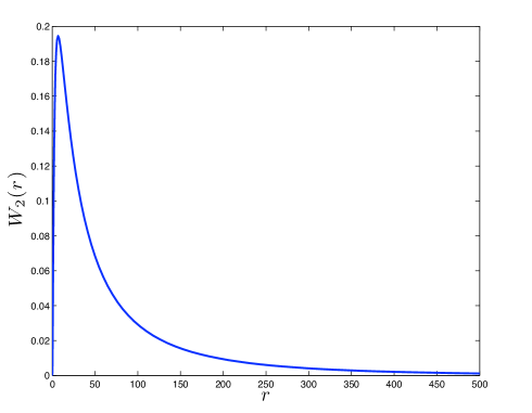
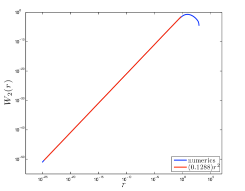
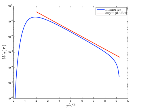
Asymptotics at small and large $r$ are known for the ground-state eigenfunction. The small-$r$ behavior was obtained by Boldyrev and Cattaneo (2004), who noted

$$W_{2}(r)=Ar^{2}+Br^{2+\xi}+o(r^{2+\xi}),\,\,\,\,\,r\ll 1.$$ (56)

Indeed, direct substitution of this ansatz shows that the Sturm-Liouville eigenvalue equation (54) is then satisfied up to terms $o(r^{\xi}),$ if and only if $B=-A.$ The large-$r$ behavior from a WKB asymptotic analysis is Vincenzi (2002); Boldyrev and Cattaneo (2004)

$$W_{2}(r)\sim\exp\left[-{{\sqrt{-2\lambda}\,r^{(2-\xi)/2}}\over{2-\xi}}\right],\,\,\,\,\,r\gg 1$$ (57)

up to a power-law prefactor. This corresponds to the dominant balance $2r^{\xi}W_{2}^{\prime\prime}\doteq-\lambda W_{2}$ in the Sturm-Liouville eq.(54) at large-$r$. Both the small-$r$ and large-$r$ asymptotic behaviors predicted analytically have been verified in our numerical solution. As shown in Fig. 2, the leading-order $r^{2}$ behavior in (56) is verified over about 24 orders of magnitude with the value $A\doteq 0.1288$ obtained by taking the small-$r$ limit of the numerical results for $W_{2}/r^{2}.$ Although we shall not show it here, we have furthermore verified the subleading $r^{10/3}$ term in (56) with the same value of $A,$ over about 16 orders of magnitude. We also verify the stretched-exponential decay (57) at large-$r$, as shown by the log-linear plot of $W_{2}(r)$ vs. $r^{1/3}$ in Fig. 3. The red line shows the slope predicted by (57) with $\lambda=-0.1927.$ Our numerical evaluation of $W_{2}(r)$ is in very good agreement with all known analytical results for the dynamo eigenfunction.

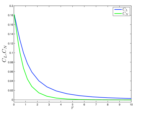
Magnetic and vector-potential correlations in the dynamo growth mode are obtained from $W_{2}$ via (36), (37) and plotted in Figs. 4 and 5 using the traditional longitudinal and transverse functions. The normalizations are those which follow from (55). One obvious feature is the much longer range of the vector-potential correlations as compared with the magnetic-field correlations.

Figure 4: Plot of magnetic field correlation functions, longitudinal $C_{L}(r)$ in blue and transverse $C_{N}(r)$ in green versus $r.$

Figure 5: Plot of magnetic vector-potential correlation functions, longitudinal $G_{L}(r)$ in blue and transverse $G_{N}(r)$ in green versus $r.$

The small-$r$ behavior is obtained from (56) to be

$$C_{L}\sim\sqrt{2}A[1-r^{\xi}+o(r^{\xi})],$$ (58)

$$C_{N}\sim\sqrt{2}A[1-(1+\frac{\xi}{2})r^{\xi}+o(r^{\xi})],$$ (59)

and

$$G_{L}\sim G_{N}\sim\frac{4\sqrt{2}A}{\lambda}[1+o(r^{\xi})].$$ (60)

Note that the contributions of order $r^{\xi}$ cancel in the latter two functions, signalling their greater smoothness. The large-$r$ behavior is found, with (57), to be

$$C_{1}\sim-\sqrt{\frac{-\lambda}{2}}r^{-\xi/2}W_{2},\,\,\,\,C_{2}\sim{{\sqrt{2}}\over{r}}W_{2}$$ (61)

$$G_{1}\sim\sqrt{\frac{2}{-\lambda}}r^{\xi/2}W_{2},\,\,\,\,G_{2}\sim\frac{2+\xi}{\sqrt{-\lambda}}r^{\xi/2}W_{2}.$$ (62)

The signs implied for $r\gg 1$ are $C_{N}<0,\,\,C_{L}>0$ and $G_{N},\,\,G_{L}>0.$ Although it is difficult to see clearly in Fig. 4, $C_{N}(r)<0$ in our numerical solution for $r>6.85.$ The existence of negative tails in $C_{N}$ was noted some time ago Ruzmaĭkin and Sokolov (1981); Novikov et al. (1983) to be a consequence of the solenoidal character of the magnetic field (see also just below).

The physical-space behaviors discussed above imply corresponding results for the magnetic energy spectrum of the dynamo mode. At low wavenumbers

$$E(k)\sim A^{\prime}k^{4},\,\,\,\,\,\,\,\,k\ll k_{\eta}$$ (63)

with $k_{\eta}=2\pi/\ell_{\eta}$ and $A^{\prime}$ some constant numerically proportional to $A.$ To see this, note that the stretched-exponential decay (61) implies that $E(k)$ is analytic at low-$k$ and can be expanded as a convergent power-series in $k^{2}.$ The leading term proportional to $k^{2}$ vanishes, however, since the integral $\int d^{3}r\,\mathcal{C}^{ij}({\bf r})=0.$ By isotropy, this is equivalent to the vanishing of the integral $\int_{0}^{\infty}dr\,r^{2}C_{T},$ where $C_{T}={{\sqrt{2}C_{1}+C_{2}}\over{r}}$ is the trace $C_{T}=C_{ii}.$ Using (36),

$$r^{2}C_{T}=\sqrt{2}\left(r\partial_{r}W_{2}+W_{2}\right)=\sqrt{2}\partial_{r}\left(rW_{2}\right),$$

so that

$$\int_{0}^{\infty}dr\,r^{2}C_{T}(r)=\sqrt{2}\lim_{r\rightarrow\infty}rW_{2}(r)=0.$$

Note that this result requires the existence of negative tails in $C_{T}$ at large $r$ Ruzmaĭkin and Sokolov (1981); Novikov et al. (1983). The $k^{4}$ spectrum in (63) was explained long ago by Kraichnan and Nagarajan Kraichnan and Nagarajan (1967) as due to the dipole magnetic field that results from “irregularly twisted and elongated current loops whose transverse dimension is $\sim k_{m}^{-1}$ [ our $k_{\eta}^{-1}$].”

The spectrum at high wavenumbers is Boldyrev and Cattaneo (2004)

$$E(k)\sim Ck^{-(1+\xi)},\,\,\,\,\,\,\,\,k\gg k_{\eta}.$$ (64)

This follows mathematically by Fourier transforming the singular terms $\propto r^{\xi}$ in (58),(59). The result (64) is the exact analogue for the Kazantsev model of the Golitsyn-Moffatt $k^{-11/3}$ spectrum Golitsyn (1960); Moffatt (1961). The dominant balance in the induction equation for length-scales $\ell\ll\ell_{\eta}$ is

$$\partial_{t}{\bf B}-\eta\triangle{\bf B}={\bf B}_{\eta}\hbox{\boldmath$\cdot$}\hbox{\boldmath$\nabla$}{\bf u},$$

with ${\bf B}_{\eta}$ the magnetic field at scale $\ell_{\eta}.$ The time-derivative must be included because of the rapid change in time of the velocity field. Solving for the statistical steady-state of the above linear Langevin equation leads to $E(k)\sim\frac{\langle B^{2}\rangle}{\eta}E_{u}(k),$ where $E_{u}(k)$ is the energy spectrum of the velocity field, and not to $E(k)\sim\frac{\langle B^{2}\rangle}{\eta^{2}k^{2}}E_{u}(k),$ as in the original argument of Golitsyn. Our discussion here exactly parallels that of Frisch and Wirth Frisch and Wirth (1996) for the analogous passive scalar problem. Note finally that the energy spectrum in the Kazantsev model, both in its low-$k$ and high-$k$ behaviors, is thus close to that argued for kinematic dynamo in inertial-range hydrodynamic turbulence by Kraichnan and Nagarajan Kraichnan and Nagarajan (1967).

Figure 6: Plot of gauge-change function $\Lambda(r)$ versus $r$.

Figure 7: Small-$r$ asymptotics of gauge-change function. In blue is a log-log plot of $\Lambda(r)-\Lambda_{0}$ versus $r$ and in red the quadratic fit $(11.93)r^{2}.$

Figure 8: Large-$r$ asymptotics of gauge-change function. In blue is a log-linear plot of $|\Lambda(r)|$ versus $r^{1/3}$ and in red a straight line with slope from (70) for $\xi=4/3$.

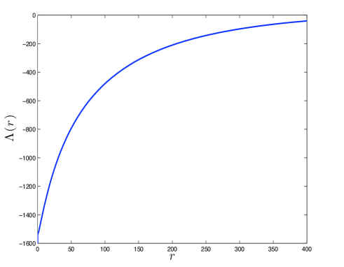
We shall now turn to the evaluation of the gauge-II correlations. For this purpose, we must determine the gauge-change function $\Lambda(r)$ which solves eq.(52):

$$r^{-2}(r^{2}b\Lambda^{\prime})^{\prime}+\lambda\Lambda=-F$$ (65)

with $F=2\Phi+TG.$ We have solved this equation numerically, by the procedure described in Appendix B. The result is plotted in Fig. 6.

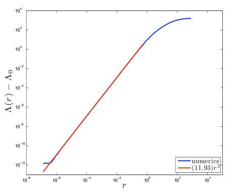
At small $r$, the solution $\Lambda=\Lambda_{reg}+\Lambda_{sing}$ is the sum of a regular part

$$\Lambda_{reg}\sim\Lambda_{0}+\Lambda_{1}r^{2}+o(r^{2})$$ (66)

and a singular part

$$\Lambda_{sing}\sim\Lambda_{s}r^{2+\xi}+o(r^{2+\xi}).$$ (67)

This is verified by substituting into eq.(65), using the similar expansion for $F$

$$F\sim F_{0}+F_{1}r^{\xi}$$

which follows from

$$\Phi=\Phi_{0}+\int_{0}^{r}d\rho\,\frac{aW_{2}}{\rho}=\Phi_{0}+O(r^{2})$$

with $\Phi_{0}=-\int_{0}^{\infty}dr\,\frac{aW_{2}}{r}<0$ and

$$TG=\frac{8\sqrt{2}A}{\lambda}\left[3+(3+\xi)r^{\xi}+o(r^{\xi})\right].$$

Thus, $F_{0}=2\Phi_{0}+\frac{24\sqrt{2}A}{\lambda}<0$ and $F_{1}=\frac{8\sqrt{2}A}{\lambda}(3+\xi)<0.$ Then it is straightforward to obtain

$$\lambda\Lambda_{0}+12\Lambda_{1}=-F_{0}$$ (68)

$$2\left[2\Lambda_{1}+(2+\xi)\Lambda_{s}\right](3+\xi)=-F_{1}.$$ (69)

These results have been verified in our numerical solution, with specific values of the constants

$$\Lambda_{0}=-1535.5,\,\,\Lambda_{1}=11.9299,\,\,\Lambda_{s}=-6.0232.$$

See Appendix B, and Fig. 7 for a comparison of $\Lambda(r)$ and $\Lambda_{reg}(r)$ at small $r.$

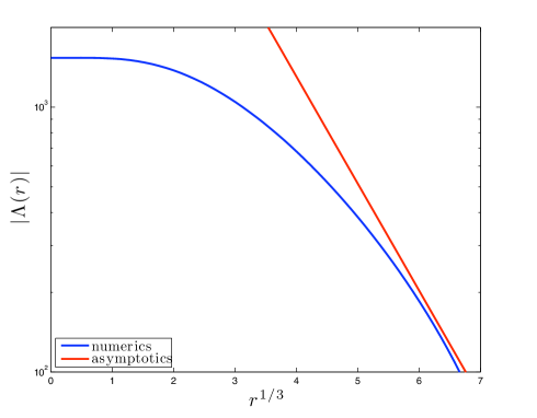
At large-$r$ we expect $\Lambda(r)\sim\exp\left[-{{\sqrt{-2\lambda}\,r^{(2-\xi)/2}}\over{2-\xi}}\right]$ up to power-law prefactors. Rewriting the eq.(65) for $\Lambda$ as

$$b\Lambda^{\prime\prime}+r^{-2}(r^{2}b)^{\prime}\Lambda^{\prime}+\lambda\Lambda=-F$$

one finds that the terms $b\Lambda^{\prime\prime},\,\,\lambda\Lambda$ cancel to leading order. For $r\gg 1.$

$$TG\sim\frac{2(2+\xi)}{\sqrt{-\lambda}}r^{3\xi/2-1}W_{2},$$

and $\Phi^{\prime}=aW_{2}/r\sim\sqrt{2}(2+\xi)r^{\xi-1}W_{2},$ so that

$$\Phi\sim-\frac{2(2+\xi)}{\sqrt{-\lambda}}r^{3\xi/2-1}W_{2}.$$

It follows that

$$F=2\Phi+TG\sim\Phi.$$

The dominant balance of $r^{-2}(r^{2}b)^{\prime}\Lambda^{\prime}$ and $-F$ gives

$$\Lambda\sim\frac{\sqrt{2}}{\lambda}r^{\xi}W_{2},\,\,\,\,\,\,\,r\gg 1.$$ (70)

This asymptotics is verified in our numerical solution. See Fig. 8 for a log-linear plot of $|\Lambda(r)|$ vs. $r^{1/3},$ with the red line having the slope predicted by (70),(57).

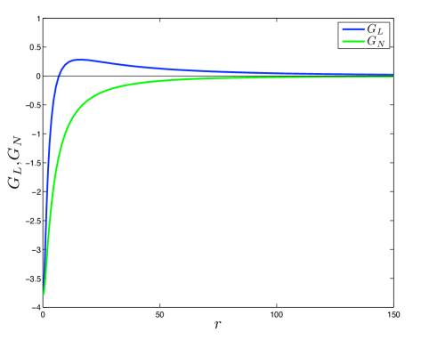
From the function $\Lambda$ we obtain $\delta\mathcal{G}$ via eq.(50). We plot in Fig. 9 the longitudinal and transverse components $\delta G_{L}$ and $\delta G_{N}$ obtained from (33). It is interesting that these functions show almost exactly opposite behaviors of algebraic signs compared with $G_{L},\,\,G_{N}$ in Fig. 5. Both $\delta G_{L}$ and $\delta G_{N}$ are proportional to $r^{\xi}$ at small $r$ because of the $\Lambda_{s}$ contribution and are stretched-exponentials

$$\delta G_{1}\sim\sqrt{\frac{2}{-\lambda}}r^{\xi/2}W_{2},\,\,\,\,\delta G_{2}\sim-\frac{r}{\sqrt{2}}W_{2}$$ (71)

at large $r,$ so that $\delta G_{N}>0,\,\,\delta G_{L}<0$ for $r\gg 1.$

Figure 9: Plot of change in vector-potential correlation functions, longitudinal $\delta G_{L}(r)$ in blue and transverse $\delta G_{N}(r)$ in green, versus $r.$

Figure 10: Plot of line-vector correlation functions, longitudinal $\widetilde{G}_{L}(r)$ in blue and transverse $\widetilde{G}_{N}(r)$ in green, versus $r.$

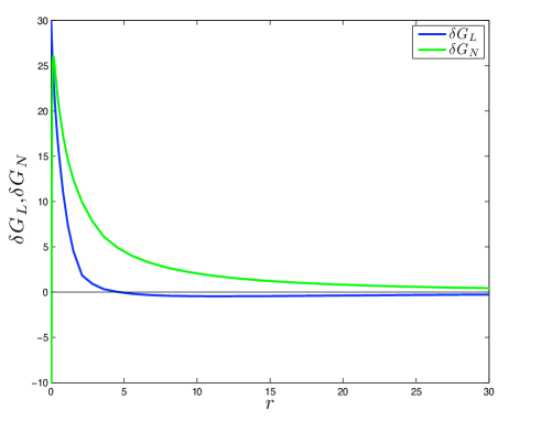
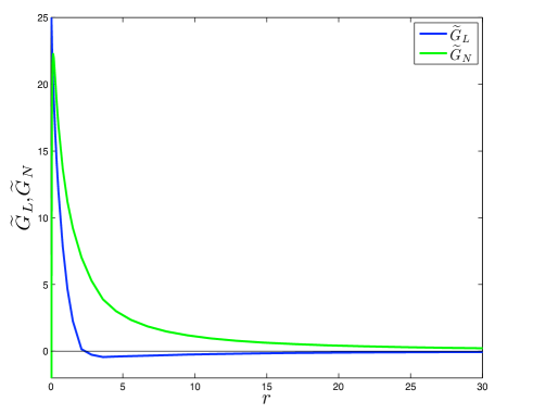
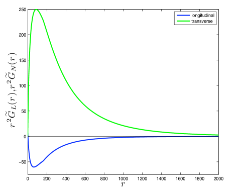
Finally, we obtain $\mathcal{\widetilde{G}}=\mathcal{G}+\delta\mathcal{G}.$ Plotted in Fig. 10 are $\widetilde{G}_{L}$, $\widetilde{G}_{N}.$ These are the central results of this paper, because of their relation to $\mathcal{R}$ in eq.(10). We can thus interpret these functions as the correlations in the dynamo growth phase of vector line-elements carried to the same final point that were initially separated by distance $r,$ with directions longitudinal and transverse to the separation vector, respectively. We shall discuss their physical interpretation below; first we consider the asymptotic behaviors for small-$r$ and large-$r$. Combining results for $\mathcal{G}$ and $\delta\mathcal{G}$ at $r\ll 1$ gives

$$\widetilde{G}_{L}\sim\left(\frac{4\sqrt{2}A}{\lambda}+2\Lambda_{1}\right)+(2+\xi)(1+\xi)\Lambda_{s}r^{\xi}$$ (72)

and

$$\widetilde{G}_{N}\sim\left(\frac{4\sqrt{2}A}{\lambda}+2\Lambda_{1}\right)+(2+\xi)\Lambda_{s}r^{\xi}.$$ (73)

It is interesting to note that $\mathcal{\widetilde{G}},$ unlike $\mathcal{G},$ contains terms $\propto r^{\xi}$ and is singular at small $r$. The reason for this is that the eq.(40) for $\widetilde{{\bf A}}$ contains the velocity-gradient $\hbox{\boldmath$\nabla$}{\bf u},$ whereas the eq.(21) for ${\bf A}$ contains only ${\bf u}$ itself. Finally, comparing the large-$r$ asymptotics in (62) with that in (71) gives for $r\gg 1$

$$\widetilde{G}_{1}\sim 2\sqrt{\frac{2}{-\lambda}}r^{\xi/2}W_{2},\,\,\,\,\widetilde{G}_{2}\sim-\frac{r}{\sqrt{2}}W_{2},$$ (74)

so that $\widetilde{G}_{N}>0,\,\,\widetilde{G}_{L}<0$ for $r\gg 1.$

The results in Fig. 10 quantify the significance of magnetic field-line stochasticity for the small-$Pr_{m}$ turbulent dynamo. The plotted correlations represent the contribution to magnetic energy at a given point produced by field vectors that arrive from points separated by distance $r$ initially. As one can see, the contribution is quite diffuse (in units of the resistive length $\ell_{\eta}$) with fat, stretched-exponential tails. Both correlations are positive for small separations $r<3\ell_{\eta}.$ Particularly interesting is the long negative tail for the longitudinal correlation $\widetilde{G}_{L},$ which represents an “anti-dynamo effect” that suppresses the turbulent growth of magnetic field energy.

Figure 11: Contribution of transverse seed field vectors to a positive line-vector correlation. Two transverse field-vectors on parallel lines at the initial time (left), when brought to the same point by a fluid motion, are positively correlated at first contact of the lines (right).

Figure 12: Contribution of longitudinal seed field vectors to a negative line-vector correlation. Two longitudinal field-vectors on the same line—or two adjacent lines— at the initial time (left), when brought to the same point by a fluid motion, are negatively correlated at first contact of the lines (right).

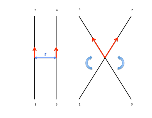
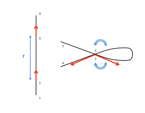
It is easy to understand the positive signs of $\widetilde{G}_{L},\,\,\widetilde{G}_{N}$ at small $r$ values. For $r\lesssim\ell_{\eta}$ the Brownian motion term dominates in the equation which follows from (1) for the relative motion ${\bf r}(t)={\bf x}_{2}(t)-{\bf x}_{1}(t)$ of a pair of points. Since the Brownian motion corresponds to a simple translation of the lines, with no rotation, the line-vectors which start parallel (either longitudinal or transverse) at separation $r\lesssim\ell_{\eta}$ will tend to remain nearly parallel when they intersect. Hence, they arrive at the final point positively correlated.

The signs of the tails of $\widetilde{G}_{L},\,\,\widetilde{G}_{N}$ for large $r$ are less easy to understand, because turbulent advection effects become important for $r\gtrsim\ell_{\eta}.$ We suggest here a heuristic explanation. In the left half of Fig. 11 we show a pair of parallel field-lines separated by ${\bf r}$ with their initially transverse line-vectors indicated in red. We then show on the right the result of a large-scale fluid motion which brings the two line-vectors together to the same point, stretched and rotated by the flow. (It is important to understand that the velocity at scales $r>\ell_{\eta}$ cannot actually bring the two lines to touch, but only within distance $\sim\ell_{\eta}$ of each other; it is then the action of two independent Brownian motions which completes their transport to the same point.) Around the time of first contact shown in the figure, the two line-vectors are positively correlated. Further rotation by the flow can eventually produce anti-alignment and negative correlation. The situation is exactly the opposite, however, for the initially longitudinal line-vectors shown in Fig. 12, which start on the same (or nearly the same) field-line. As these vectors are brought together by a similar fluid motion as before, the line vectors are anti-aligned near the time of first contact. They may then become positively oriented as further rotation and stretching occurs. These geometric considerations may help to explain why, for large enough $r,$ positive alignment dominates in $\widetilde{G}_{N}$ while negative alignment dominates in $\widetilde{G}_{L}.$ Transverse line-vectors seem to be brought together from large distances by mainly lateral advection of field-lines, while longitudinal vectors are brought together by twisting and looping of field-lines.

IV Uniform Fields and Magnetic Induction

We now turn to the second question left open in I, the fate of spatially-uniform magnetic seed fields in the dynamo regime of the Kazantsev model. This issue is closely related to the problem of “magnetic induction”, which is often defined simply as the generation of small-scale magnetic fluctuations by turbulent tangling of the lines of a non-vanishing mean-field. In the case of homogeneous statistics—which we only consider in this paper—any non-zero average field must be spatially uniform. Thus, the response of a uniform field to homogeneous turbulence is intimately related to that of magnetic induction. In fact, we shall argue that there is no real distinction in this context between “magnetic induction” and “fluctuation dynamo” with a uniform seed field.

Let us consider then the special case that the initial magnetic-field ${\bf B}_{(0)}$ is spatially-uniform (but still possibly random). Applying eq.(11) gives the energy in the fluctuation field ${\bf b}={\bf B}-\langle{\bf B}\rangle$ to be

$$\langle b^{2}(t)\rangle=\mathcal{R}_{k\ell}(t)\langle B^{k}_{(0)}B^{\ell}_{(0)}\rangle-\delta_{k\ell}\langle B^{k}_{(0)}\rangle\langle B^{\ell}_{(0)}\rangle$$ (75)

$$=\mathcal{R}_{k\ell}(t)\langle b^{k}_{(0)}b^{\ell}_{(0)}\rangle+[\mathcal{R}_{k\ell}(t)-\delta_{k\ell}]\langle B^{k}_{(0)}\rangle\langle B^{\ell}_{(0)}\rangle.\,\,\,\,\,\,\,\,$$ (76)

In the second line of the equation above, one may make a formal distinction between “fluctuation dynamo” represented by the first term and “magnetic induction” represented by the second term. However, their asymptotic growth rates at long times are the same, both given by

$$\mathcal{R}_{k\ell}(t)\sim e^{-\lambda t}\mathcal{\widetilde{G}}_{k\ell},\,\,\,\,\,\,\,\,\,\,\,\,(\lambda<0)$$

if the integral

$$\mathcal{\widetilde{G}}_{k\ell}\equiv\int d^{3}r\,\,\mathcal{\widetilde{G}}_{k\ell}({\bf r})$$

is non-vanishing. We show now that it is indeed non-zero.

Since the above integral is gauge-invariant, one may just as well consider the integral of $\mathcal{G}_{k\ell}({\bf r}).$ Furthermore, as long as the turbulent velocity field (but not necessarily the magnetic field) is statistically isotropic, then

$$\mathcal{G}_{k\ell}=\int d^{3}r\,\,\mathcal{G}_{k\ell}({\bf r})=\frac{1}{3}G_{T}\delta_{k\ell}$$

where $G_{T}\equiv 4\pi\int_{0}^{\infty}dr\,r^{2}G_{T}(r)$ and $G_{T}(r)=G_{L}(r)+2G_{N}(r)$ is the trace function. From (37)

$$G_{T}(r)={{\sqrt{2}G_{1}+G_{2}}\over{r}}={{2aW_{2}+(a+\sqrt{2}b)r\partial_{r}W_{2}}\over{\lambda r^{2}}}.$$

Using the incompressibility condition $a=\sqrt{2}\left(b+{{1}\over{2}}rb^{\prime}\right)$ and integrating by parts once in $r$ gives

$$\int_{0}^{\infty}dr\,r^{2}G_{T}(r)=-{{1}\over\sqrt{2}\lambda}\int_{0}^{\infty}(r^{2}b^{\prime\prime}+4rb^{\prime})W_{2}(r)\,dr.$$

On the other hand, multiplying the eigenvalue equation (38) by $r^{2}$ and integrating by parts in $r$ twice gives

$$-\int_{0}^{\infty}(r^{2}b^{\prime\prime}+4rb^{\prime})W_{2}(r)\,dr=\lambda\int_{0}^{\infty}r^{2}W_{2}(r)\,dr.$$

We finally obtain that

$$G_{T}\equiv 4\pi\int_{0}^{\infty}dr\,r^{2}G_{T}(r)=2\pi\sqrt{2}\int_{0}^{\infty}r^{2}W_{2}(r)\,dr>0.$$

We used here the positivity of the ground-state (dynamo) eigenfunction $W_{2}$. Notice that we have not assumed any specific form of $b(r),$ as long as the dynamo mode exists.

In fact, the entire spatial structure of small-scale fluctuations for “magnetic induction” is the same as that for “fluctuation dynamo” at long times. Both are determined by the same dynamo eigenmode. To see this, we note that the magnetic correlation can be expanded, in general, into right eigenmodes of $\mathcal{M}:$

$$\mathcal{C}^{ij}({\bf r},t)=\sum_{\alpha}c_{\alpha}e^{-\lambda_{\alpha}t}\mathcal{C}^{ij}_{\alpha}({\bf r})$$ (77)

The expansion coefficients are determined from the initial correlation $\mathcal{C}^{ij}_{(0)}({\bf r})$ by

$$c_{\alpha}\equiv\int d^{3}r\,\,\mathcal{G}_{\alpha;ij}({\bf r})\mathcal{C}^{ij}_{(0)}({\bf r}),$$ (78)

using biorthogonality of right and left eigenmodes $\mathcal{C}_{\alpha}$ and $\mathcal{G}_{\alpha}$. If $\mathcal{C}^{ij}_{(0)}({\bf r})=\langle B^{i}_{(0)}B^{j}_{(0)}\rangle$ is ${\bf r}$-independent, then for the ground state mode (say $\alpha=0$) $c_{0}=\mathcal{G}_{0;k\ell}\langle B^{k}_{(0)}B^{\ell}_{(0)}\rangle=\frac{1}{3}G_{T}\langle B_{(0)}^{2}\rangle>0.$ Thus, with $r$ fixed,

$$\mathcal{C}^{ij}({\bf r},t)\sim c_{0}e^{-\lambda_{0}t}\mathcal{C}^{ij}_{0}({\bf r}),\,\,\,\,\,\,\,\,t\rightarrow\infty.$$

The magnetic correlation $\mathcal{C}^{ij}({\bf r},t)$ is dominated by the leading dynamo eigenmode $\mathcal{C}^{ij}_{0}({\bf r})$ with subleading contributions from additional eigenmodes (point spectrum of $\mathcal{M}$) if any. There is no essential physical difference between the two cases of “fluctuation dynamo” (${\bf B}_{(0)}={\bf b}_{(0)}$) and “magnetic induction” (${\bf B}_{(0)}=\langle{\bf B}_{(0)}\rangle$).

It is interesting to consider in (77) also the opposite limit of large $r$ with $t$ fixed. In that case, the result with initial condition $\mathcal{C}^{ij}_{(0)}({\bf r})=\langle B^{i}_{(0)}B^{j}_{(0)}\rangle$ is

$$\mathcal{C}^{ij}({\bf r},t)\sim\langle B^{i}_{(0)}B^{j}_{(0)}\rangle,\,\,\,\,\,\,\,\,r\rightarrow\infty.$$ (79)

This is clearly true for the case $\mathcal{C}^{ij}_{(0)}({\bf r})=\langle B^{i}_{(0)}\rangle\langle B^{j}_{(0)}\rangle,$ because the above limit then corresponds to “clustering” of the magnetic correlation function. However, the expansion coefficients (78) are linear in the initial correlation, so the above result must hold whenever $\mathcal{C}_{(0)}^{ij}({\bf r})$ is ${\bf r}$-independent. The limit (79) comes entirely from the continuous spectrum of $\mathcal{M}$ in the expansion (77) (for which the sum over $\alpha$ is actually an integral), because the finite number of dynamo eigenmodes $\mathcal{C}_{\alpha}$ associated to the point spectrum of $\mathcal{M}$ all have the stretched-exponential decay in (57), with the corresponding value of $\lambda_{\alpha}<0$. Their contribution thus vanishes in the large-$r$ limit.

We conclude that there is no essential distinction in the dynamo regime between “magnetic induction” for a uniform mean-field and “fluctuation dynamo” for a homogeneous (but random) seed field, since all of their physical behaviors and underlying mechanisms are exactly the same. Another possible definition of “magnetic induction” which is employed in the literature is the growth of small-scale fluctuation fields generated from a non-vanishing mean-field, but only in a parameter regime where the “fluctuation dynamo” does not exist. The term is used this way in discussion of liquid-metal laboratory experiments operated at a sub-threshold regime Peffley et al. (2000); Bourgoin et al. (2002); Nornberg et al. (2006). Although such inductive growth of fluctuations is generally sub-exponential, it may be exponential if the average magnetic field is itself exponentially growing because of a mean-field dynamo effect. Of course, with this definition, it makes no sense to regard “magnetic induction” and “fluctuation dynamo” as possible co-existing and competing mechanisms for small-scale magnetic field growth.

We may consider as an example of this second type of “magnetic induction” the failed-dynamo regime of the KK model for $\xi<1,$ at zero Prandtl number and infinite magnetic Reynolds number. Unlike the liquid-metal experiments where fluctuation-dynamo fails because $Re_{m}<Re_{m}^{(c)},$ the failure here is due to the extreme roughness of the advecting velocity field (see I). This model problem is not a perfect analogue of the induction phenenoma seen in the experiments. For example, we solve the KK model with velocity integral scale $L=\infty$ (and thus $Re_{m}=\infty$) so that the large-scales of our problem are quite different than the non-universal, inhomogeneous and anisotropic conditions seen in experiments. Also, the average field is uniform in the KK model with homogeneous statistics. Since spatially constant fields must be time-independent, we cannot study in this setting induction of an exponentially growing mean-field. On the other hand, the cited experiments Peffley et al. (2000); Bourgoin et al. (2002); Nornberg et al. (2006) have studied the turbulent induction of a near-uniform, stationary external field. The analogy with those experiments is close enough that we can test some proposed theories of “magnetic induction” in our model situation.

We therefore consider in this light several results of I for the failed dynamo regime of the KK model with $\xi<1.$ It was found there for the case of spatially-uniform and isotropic initial data $\mathcal{C}^{ij}_{(0)}({\bf r})=A\delta^{ij}$ that, at long times,

$$\langle B^{2}(t)\rangle\propto\ell_{\eta}^{\zeta_{1}}(D_{1}t)^{|\zeta_{1}|/\gamma},$$ (80)

with

$$\zeta_{1}=-\frac{3}{2}-\frac{\xi}{2}+\frac{3}{2}\sqrt{1-\frac{1}{3}\xi(\xi+2)}$$

which is negative and decreasing from 0 to $-2$ for $0<\xi<1.$ Thus, the energy in the magnetic fluctuations is growing, but only as a power-law in $t$. These same results hold , in fact, for general uniform initial data of the form $\mathcal{C}^{ij}_{(0)}({\bf r})=\langle B^{i}_{(0)}B^{j}_{(0)}\rangle.$ This follows directly from eq.(11) when the random velocity (but not necessarily the magnetic field) is statistically isotropic and the line-correlation matrix $\mathcal{R}_{k\ell}(t)=\frac{1}{3}\mathcal{R}(t)\delta_{k\ell}.$

Paper I showed further that there are three spatial regimes of the magnetic correlation. These are the resistive range:

$$C_{L}(r,t)\simeq A^{\prime\prime}\left(\frac{\ell_{\eta}}{L(t)}\right)^{\zeta_{1}}\left[1-2\left(\frac{r}{\ell_{\eta}}\right)^{\xi}\right]\,\,\,\,r\ll\ell_{\eta},$$ (81)

the quasi-steady, inertial-convective range:

$$C_{L}(r,t)\simeq A^{\prime}\left(\frac{r}{L(t)}\right)^{\zeta_{1}}\,\,\,\,\ell_{\eta}\ll r\ll L(t),$$ (82)

and the very large-scale range:

$$C_{L}(r,t)\simeq A\left[1-\frac{2\zeta_{1}(\zeta_{1}+3+\xi)}{\gamma}\left(\frac{L(t)}{r}\right)^{\gamma}\right]\,\,\,\,r\gg L(t).$$ (83)

We have here defined $L(t)\equiv(D_{1}t)^{1/\gamma}$ to be a characteristic large length-scale of the magnetic field. Note that $A^{\prime},A^{\prime\prime}$ are constants numerically proportional to $A.$ Result (81) follows from the formula for $\Gamma_{in}(\sigma)$ on p.26 of I, together with the series expansion of the hypergeometric function ${\,\!}_{2}F_{1}$ (eq.(75) in I). Equations (82) and (83) follow from I, eq.(67) for $\alpha=0$ with $\rho\ll 1$ and $\rho\gg 1,$ respectively. For the last case, the large-argument asymptotics of the Kummer function in Erdélyi (1953), eq. 6.13.1(2), is employed to derive the $1/r^{\gamma}$ term.

These three ranges all have simple physical descriptions, which are easiest to discuss based on the corresponding magnetic energy spectra obtained by Fourier transform. In the resistive range the result is

$$E(k,t)\propto\frac{\langle B^{2}(t)\rangle}{\eta}k^{-(1+\xi)}\,\,\,\,\,\,\,\,\,k\gg k_{\eta}.$$ (84)

(Note that $\eta=D_{1}\ell_{\eta}^{\xi}.$) This is a Golitsyn-like spectrum, with physics exactly like that discussed earlier for the resistive range of the dynamo growth modes. This range is very universal in the small-$Pr_{m}$ limit.

The inertial-convective range has energy spectrum

$$E(k,t)\simeq A^{\prime}[L(t)]^{|\zeta_{1}|}k^{|\zeta_{1}|-1}\,\,\,\,\,\,\,\,\,k_{L}(t)\ll k\ll k_{\eta}$$ (85)

with $k_{L}(t)=2\pi/L(t)\rightarrow 0$ as $t\rightarrow\infty.$ This growing range is responsible for the energy increase in (80). It is “quasi-steady” in the sense that all its statistical characteristics are identical to those in the forced steady-state (see Vergassola (1996) and I), with the uniform initial field replacing the role of the external force. The physics involves a nontrivial competition of stretching ${\bf B}\hbox{\boldmath$\cdot$}\hbox{\boldmath$\nabla$}{\bf u}$ and nonlinear cascade ${\bf u}\hbox{\boldmath$\cdot$}\hbox{\boldmath$\nabla$}{\bf b}.$ If one assumes that “induction” of the initial, background field ${\bf B}_{(0)}\hbox{\boldmath$\cdot$}\hbox{\boldmath$\nabla$}{\bf u}$ dominates the stretching, then this is the same physics invoked by Ruzmaĭkin and Shukurov Ruzmaĭkin and Shukurov (1982) for induced fluctuations. Assuming a balance of the terms $({\bf u}\hbox{\boldmath$\cdot$}\hbox{\boldmath$\nabla$}){\bf b}\simeq{\bf b}\hbox{\boldmath$\cdot$}\hbox{\boldmath$\nabla$}{\bf u}\simeq{\bf B}_{(0)}\hbox{\boldmath$\cdot$}\hbox{\boldmath$\nabla$}{\bf u},$ they proposed on dimensional grounds an $Ak^{-1}$ spectrum, with $A\propto\langle B^{2}_{(0)}\rangle.$ However, such a spectrum only occurs in the KK model for $\xi=0.$ In that case, the cascade term ${\bf u}\hbox{\boldmath$\cdot$}\hbox{\boldmath$\nabla$}{\bf b}$ can be represented as an eddy-diffusivity $2D_{1}$ and a balance equation

$$\partial_{t}{\bf b}-2D_{1}\triangle{\bf b}={\bf B}_{(0)}\hbox{\boldmath$\cdot$}\hbox{\boldmath$\nabla$}{\bf u}$$

predicts the correct spectrum $\langle B_{(0)}^{2}\rangle k^{-1}.$ There is no distinction in this case between the inertial-convective range and the resistive range with Golitsyn spectrum. For $0<\xi<1,$ however, there is an “anomalous dimension” $|\zeta_{1}|$ which corrects the dimensional prediction. There is no longer any simple, heuristic argument for the magnetic spectral exponent in the quasi-steady range, which requires the computation of a non-perturbative zero-mode. The physics involves a nontrivial competition between creation of magnetic energy by stretching and destruction by turbulent cascade to the resistive range.

For the very low wavenumber range $k\ll k_{L}(t)$ one might expect the dimensional argument of Ruzmaĭkin and Shukurov to work after all and to correctly yield an $Ak^{-1}$ spectrum. The results in (81)-(83) correspond to a member of the one-parameter family of self-similar decay solutions found in I, with parameter choice $\alpha=0.$ For the general member of this family, the low-wavenumber spectrum is of the form $Ak^{\alpha-1}$ (“permanence of large eddies”; see I), so setting $\alpha=0$ should naively lead to the Ruzmaĭkin-Shukurov prediction. But this is not the case. Fourier transformation of the initial uniform magnetic field instead yields a term in the energy spectrum $\propto A\delta(k),$ a delta-function at $k=0.$ The actual energy spectrum in the low-wavenumber range is found by Fourier transforming the second term in (83) to be

$$E(k,t)\simeq A^{\prime}[L(t)]^{\gamma}k^{1-\xi},\,\,\,\,\,\,\,\,\,k\ll k_{L}(t).$$ (86)

The simple physics of this range is direct induction from the spatially-constant field via the balance

$$\partial_{t}{\bf b}={\bf B}_{(0)}\hbox{\boldmath$\cdot$}\hbox{\boldmath$\nabla$}{\bf u}.$$

Indeed, solving this linear Langevin equation yields $E(k,t)\propto\langle B^{2}_{(0)}\rangle(D_{1}t)k^{2}E_{u}(k),$ reproducing the above spectrum. Note that $[L(t)]^{\gamma}=D_{1}t$ corresponds to diffusive spectral growth in this range, due to the white-noise in time character of the advecting velocity field. The total energy in this range remains constant in time, however, because shrinking of the range exactly compensates for increase of the energy spectrum. Once the energy $b_{k}^{2}\simeq kE(k,t)$ in an interval around wavenumber $k$ approaches the energy $\langle B_{(0)}^{2}\rangle$ in the initial uniform field a nonlinear cascade begins and that wavenumber $k$ joins the inertial-convective range with spectrum (85).

The above argument resembles one which has been invoked to explain a $k^{-5/3}$ spectrum of magnetic energy reported at wavenumbers $k<k_{\eta}$ in some low-$Pr_{m}$ liquid-metal experiments Peffley et al. (2000); Nornberg et al. (2006) and in a related numerical simulation Bayliss et al. (2007). These works study the induction of an imposed magnetic field by a turbulent flow with a Kolmogorov energy spectrum. The argument made by those authors amounts to assuming a balance between induction of the external magnetic field ${\bf B}_{(0)}$ and convection by the large-scale velocity ${\bf u}_{(0)}$ (both mean and fluctuating components):

$${\bf u}_{(0)}\hbox{\boldmath$\cdot$}\hbox{\boldmath$\nabla$}{\bf b}={\bf B}_{(0)}\hbox{\boldmath$\cdot$}\hbox{\boldmath$\nabla$}{\bf u}.$$

This leads to the prediction that $\langle u_{(0)}^{2}\rangle E(k)\simeq\langle B_{(0)}^{2}\rangle E_{u}(k),$ so that $E_{u}(k)\simeq\varepsilon^{2/3}k^{-5/3}$ implies a similar magnetic energy spectrum $E(k)$. We find this argument unconvincing. In the first place, large-scale advection conserves the energy in magnetic fluctuations. It cannot therefore balance the input from induction of ${\bf B}_{(0)}.$ If nonlinear cascade can be ignored, then magnetic energy must be expected to grow, as in our result (86) above, and not to saturate. Furthermore, if the large-scale sweeping were important, then it should appear in our balance argument for (86), because the KK model contains such dynamical sweeping effects. However, we see that the correct spectrum at very low wavenumbers is obtained by ignoring such sweeping as irrelevant. This is consistent with the results of Frisch and Wirth Frisch and Wirth (1996) for the diffusive range of a passive scalar, who emphasized the (nontrivial) fact that sweeping by large-scales plays no role in the balance for that high-wavenumber range. Finally, we note that $k^{-5/3}$ is the (Obukhov-Corrsin) spectrum expected for a passive scalar in a Kolmogorov inertial-range and not for a passive magnetic field. The argument of Peffley et al. (2000); Nornberg et al. (2006); Bayliss et al. (2007) thus omits the effects of the small-scale stretching interaction $({\bf b}\hbox{\boldmath$\cdot$}\hbox{\boldmath$\nabla$}){\bf u}$ and we know of no good justification for doing so in a steady-state, saturated regime.

V Conclusions

The main purpose of this paper was to quantify the importance of stochasticity of flux-line freezing to the zero-Prandtl-number turbulent dynamo. It is a rigorous result for the Kazantsev-Kraichnan model that Lagrangian trajectories becomes intrinsically stochastic in the inertial range with velocity roughness exponent $\xi$, due to Richardson 2-particle turbulent diffusion. In this situation, infinitely-many magnetic lines in the initial seed field at time $t_{0}$ are brought to a point at time $t$ from a region of size $L(t)\sim(t-t_{0})^{1/(2-\xi)}.$ Note that the size of the region sampled is independent of the resistivity. Not all of the magnetic field lines in this large region will, however, make an equal contribution to the net dynamo growth of magnetic energy. The contribution from lines initially separated by distance $r$ is quantified, in isotropic non-helical turbulence, by the line-correlations $R_{L}(r,t)$ and $R_{N}(r,t).$ At long times, these correlations are proportional to $e^{-\lambda t}\widetilde{G}_{L}(r)$ and $e^{-t\lambda t}\widetilde{G}_{N}(r),$ respectively, where $\widetilde{G}_{L}(r)$ and $\widetilde{G}_{N}(r)$ are longitudinal and transverse components of the (left/adjoint) dynamo eigenfunction. The central results of this paper are these two functions, plotted in Fig. 10, which quantify the relative contribution to magnetic energy from lines initially separated by the distance $r,$ in resistive units.

The principal contribution to the dynamo growth comes from lines at separations of the order of magnitude of the resistive length $\ell_{\eta}.$ However, the decay of the correlations, in units of the resistive length, is a slow, stretched exponential. This implies that lines which arrive from any arbitrary, fixed separation $r$—no matter how large—will contribute an amount of energy growing exponentially rapidly in time. Of course lines separated by $r$ much, much greater than $\ell_{\eta}$ will make a small relative contribution, but even lines separated by many $\ell_{\eta}$ make a substantial contribution. To underline this fact, we plot in Fig. 13 below the eigenfunctions $\widetilde{G}_{L}(r)$ and $\widetilde{G}_{N}(r)$ multiplied by $r^{2},$ which, integrated over $r,$ give the mean magnetic energy for a uniform seed field. (In order to make this plot, we have extended our numerical results to $r>163\ell_{\eta}$ with the asymptotic formulas (74).) As this figure should make clear, lines separated by many hundreds of resistive lengths are important to the dynamo growth. To be more quantitative, we find that lines initially separated by up to $968\ell_{\eta}$ must be considered in order to get 90% of the total magnetic energy. Another feature dramatically illustrated in Fig. 13 is the strong anti-dynamo effect arising from lines-vectors initially parallel to the separation vector ${\bf r}$, represented by the long negative tail in $r^{2}\widetilde{G}_{L}(r).$ We have proposed a heuristic explanation for this interesting effect in terms of twisting and looping of field lines (Figs. 11 and 12).

Figure 13: Contributions of line-correlations to the energy. The integrands, $r^{2}\,G_{L}(r)$ in blue and $r^{2}\,G_{N}(r)$ in green, for magnetic energy with a uniform seed field in eqs.(11),(12).

As we shall see in a following paper Eyink (2010) these principle conclusions apply not only in the Kazantsev-Kraichnan model with $Pr_{m}=0$ but also to kinematic dynamo in real hydrodynamic turbulence with $Pr_{m}\sim 1.$

A second purpose of this paper was to discuss the meaningful distinction, if any, between “fluctuation dynamo” and “magnetic induction.” In the case of the KK model at $Pr_{m}=0$ and $Re_{m}=\infty,$ we have shown that a uniform mean field (or a uniform random field) may provide the seed field for small-scale fluctuation dynamo. The asymptotic exponential growth rate and the small-scale magnetic correlations are exactly the same as for any other random seed field whose correlation function is non-orthogonal to the leading dynamo mode. We therefore do not agree with authors Brandenburg and Subramanian (2005); Schekochihin et al. (2007); Schüssler and Vögler (2008) who distinguish between “fluctuation dynamo” and “magnetic induction” as two fundamentally different mechanisms.

For example, Schüssler and Vögler Schüssler and Vögler (2008) have proposed to explain small-scale magnetic fields in the quiet solar photosphere as a consequence of near-surface dynamo action. They mention magnetic induction as a possible alternative explanation, but dismiss it with the remark: “ ‘Shredding’ of pre-existing magnetic flux (remnants of bipolar magnetic regions) cannot explain the large amount of observed horizontal flux since the turbulent cascade does not lead to an accumulation of energy (and generation of a spectral maximum) at small scales. On the other hand, such a behavior is typical for turbulent dynamo action.” We find in the KK model that, quite to the contrary, induction of a mean field produces the same small-scale fluctuations and energy spectra as does the fluctuation dynamo. We may indeed say that—at least in the kinematic regime of weak fields— “magnetic induction” is nothing but “fluctuation dynamo” with a large-scale, deterministic (mean) seed field.

Although Schekochihin et al. Schekochihin et al. (2007) do make a distinction between two separate mechanisms, their final conclusion is not so different from ours. In their Fig. 8(a) they find, in a sub-threshold regime with $Re_{m}<Re_{m}^{(c)},$ that saturated energy spectra for induction from a uniform field and for decaying spectra of the “failed” dynamo state exactly coincide, when normalized to the same total energy. They conclude that “the same mechanism is responsible for setting the shape of the spectrum of the magnetic fluctuations induced by a mean field and of the decaying or growing such fluctuations in the absence of a mean field,” just as we see in the KK model.

We have also studied the KK model with velocity roughness exponent $\xi<1,$ where the $Pr_{m}=0$ fluctuation dynamo does not exist, and with a uniform magnetic seed field in order to get some insight into the physics of the induction mechanism in a failed-dyamo regime. This is very roughly the same situation that was studied in several liquid-sodium experiments with $Pr_{m}\lesssim 10^{-5}$ Odier et al. (1998); Bourgoin et al. (2002); Peffley et al. (2000); Spence et al. (2006); Nornberg et al. (2006) and in related numerical simulations Bayliss et al. (2007); Schekochihin et al. (2007) at somewhat larger Prandtl numbers. Some of those studies have reported observing a $k^{-5/3}$ spectrum of magnetic fluctuations in the velocity inertial-range Peffley et al. (2000); Nornberg et al. (2006); Bayliss et al. (2007), while others have reported a $k^{-1}$ spectrum Bourgoin et al. (2002); Schekochihin et al. (2007). The very least we can conclude from our analysis is that the explanations offered for those spectra based on inertial-range turbulence physics do not successfully explain the results in the KK model, even where those explanations should apparently apply. An exception is the Golitsyn-Moffatt argument for the spectrum at wavenumbers $k>k_{\eta},$ which succeeds (with slight modification) in the KK model. At intermediate wavenumbers $k_{L}(t)<k<k_{\eta},$ we find in the KK model a range with input of magnetic energy by induction of the mean field balanced by nonlinear stretching and cascade to the resistive scale. This is the same physics invoked in the theory of Ruzmaĭkin and Shukurov Ruzmaĭkin and Shukurov (1982), who predicted a spectrum $\langle B^{2}_{0}\rangle k^{-1}$ on dimensional grounds. However, this prediction is only verified in the KK model for $\xi=0,$ where nonlinear cascade can be accurately modelled as an eddy-diffusivity. For the KK model with $0<\xi<1$ this prediction is modified by a large anomalous exponent $|\zeta_{1}|$ (with $|\zeta_{1}|=2$ for $\xi=1$) which must be calculated by a non-perturbative argument. At low wavenumbers $k<k_{L}(t)$ in the KK model we find a range with continuous growth of magnetic energy spectrum supplied by induction of the uniform field. Unlike the argument in Peffley et al. (2000); Nornberg et al. (2006); Bayliss et al. (2007), there is no balance with large-scale advection, although such effects exist in the model. Indeed, it is very unclear to us how large-scale advection, which conserves magnetic energy, can by itself balance the input from induction.

We shall not attempt here to explain in detail the induced spectra observed in the experiments and simulations, except to note that they must involve large-scale physics outside inertial-range scales. This was, in fact, the point of view of Bourgoin et al. Bourgoin et al. (2002) who explained their $k^{-1}$ spectrum by global fluctuations of the flow pattern. Large-scale effects are certainly necessary to obtain saturation of the energy. If the length-scale $L(t)$ in (85) had a finite limit for large times, e.g. for turbulence confined to a box of size $L_{B},$ then the system should reach a statistical steady-state, just as in the randomly-forced case Vergassola (1996). Otherwise, magnetic energy would continue to grow without bound within a kinematic description. In such a steady-state, the only extended spectral ranges would be the nonlinear range (85) and the Golitsyn range (84). The latter is well-confirmed in experiments Odier et al. (1998); Bourgoin et al. (2002); Nornberg et al. (2006) and simulations Bayliss et al. (2007); Schekochihin et al. (2007). If the $k^{-1}$ or $k^{-5/3}$ spectra observed at larger scales can be understood at all in terms of inertial-range turbulence, then it seems that an analogue of the nonlinear range (85) is the most likely explanation. If so, then the determination of the precise exponent is a hard theoretical problem, for there may be large anomalous scaling corrections to the dimensional Ruzmaĭkin-Shukurov $k^{-1}$ spectrum.

The precise spectral exponent of induced magnetic fluctuations in the liquid metal experiments is open to debate. Over the limited scaling ranges available it is quite difficult to distinguish between $-5/3$ and $-1$ exponents and the empirical spectra can be fit about equally well with both power-laws, or others as well. It is not even clear that the concept of “scaling exponent” is entirely well-defined without the possibility to extend the putative scaling ranges. Our three spectral ranges (84), (85),(86) can be made arbitrarily long by adjusting parameters, but, in the experiments and simulations, only the Golitsyn spectral range can be lengthened by lowering $Pr_{m}.$ The low-wavenumber spectral ranges can be made longer only by increasing $Re_{m},$ but, beyond a critical value $Re_{m}^{(c)},$ the dynamo effect sets in and the physical phenomena change.

Appendix A Boldyrev-Cattaneo-Rosner formalism

We consider in this appendix kinematical relations between the two-point correlations of magnetic fields and vector potentials, first for spatially homogeneous ensembles and then for both homogeneous and isotropic ensembles (but not reflection-symmetric). The results are closely related to those in classical references on homogeneous turbulence, such as Batchelor (1953) and Monin and Yaglom (1975), but we employ a mathematical reformulation of Boldyrev et al. (2005) (hereafter, BCR) that was developed for helical turbulence. We discuss here, in particular, the consequences of gauge-invariance.

The two-point correlation of the magnetic field in a homogeneous ensemble is defined as $\mathcal{C}^{ij}({\bf r},t)=\langle B^{i}({\bf r},t)B^{j}(\hbox{\boldmath$0$},t)\rangle.$ This satisfies the solenoidality conditions $\partial_{i}\mathcal{C}^{ij}=\partial_{j}\mathcal{C}^{ij}=0.$ The two-point correlation of the magnetic vector-potential is likewise $\mathcal{G}_{ij}({\bf r},t)=\langle A_{i}({\bf r},t)A_{j}(\hbox{\boldmath$0$},t)\rangle$. A pure gauge field $A_{i}^{g}=\partial_{i}\lambda$ has correlation $\mathcal{G}_{ij}^{g}=-\partial_{i}\partial_{j}\Lambda$ with $\Lambda({\bf r})=\langle\lambda({\bf r})\lambda(\hbox{\boldmath$0$})\rangle.$ Solenoidal correlations $\mathcal{C}$ and pure-gauge correlations $\mathcal{G}^{g}$ form mutually orthogonal subspaces in the Hilbert space with inner product

$$\langle\mathcal{C},\mathcal{G}\rangle=\int d^{d}r\,\mathcal{C}^{ij}({\bf r})\mathcal{G}_{ij}({\bf r}).$$ (87)

This observation will prove important in what follows. Notice also that the magnetic and vector-potential fields are related by curls, so that

$$\mathcal{C}^{ij}=-\mathcal{D}^{ij,k\ell}\mathcal{G}_{k\ell}$$

with the non-positive, self-adjoint differential operator

$$\mathcal{D}^{ij,k\ell}=\epsilon^{ikp}\epsilon^{j\ell q}\partial_{p}\partial_{q}.$$

It is furthermore useful to introduce the joint correlations of magnetic fields and vector-potentials

$$\Psi^{i\,\,\,\,}_{\,\,\,\,k}({\bf r},t)=\langle B^{i}({\bf r},t)A_{k}(\hbox{\boldmath$0$},t)\rangle,\,\,\Psi_{k\,\,\,\,}^{\,\,\,\,i}({\bf r},t)=\langle A_{k}({\bf r},t)B^{i}(\hbox{\boldmath$0$},t)\rangle$$

which are related by $\Psi^{i\,\,\,\,}_{\,\,\,\,k}({\bf r},t)=\Psi_{k\,\,\,\,}^{\,\,\,\,i}(-{\bf r},t).$ These are obtained from the vector-potential correlation by

$$\Psi^{i\,\,\,\,}_{\,\,\,\,\ell}=\mathcal{R}^{i,k}\mathcal{G}_{k\ell}$$

with

$$\mathcal{R}^{i,k}=\epsilon^{ipk}\partial_{p},$$

and likewise

$$\Psi_{k\,\,\,\,}^{\,\,\,\,j}=-\mathcal{R}^{j,\ell}\mathcal{G}_{k\ell}=(\mathcal{R}^{j,\ell})^{*}\mathcal{G}_{k\ell}.$$

The symbol * here denotes adjoint with respect to $\langle f,g\rangle=\int d^{3}r\,f({\bf r})g({\bf r}).$ Note that $\mathcal{D}^{ij,k\ell}=-\mathcal{R}^{i,k}(\mathcal{R}^{j,\ell})^{*}.$

We are mainly concerned with statistics both homogeneous and isotropic, but not necessarily invariant under space reflections. In that case, the magnetic correlation becomes

$$\mathcal{C}^{ij}({\bf r},t)=C_{L}\hat{r}^{i}\hat{r}^{j}+C_{N}(\delta^{ij}-\hat{r}^{i}\hat{r}^{j})+C_{H}\epsilon^{ijk}\hat{r}_{k},$$

with coefficients depending only on $r,t,$ and the solenoidal condition becomes

$$C_{N}(r,t)=C_{L}(r,r)+\frac{1}{2}rC_{L}^{\prime}(r,t).$$

Note that there is no condition on $C_{H},$ as the third term is always divergence-free. One can similarly write the vector-potential correlation as

$$\mathcal{G}_{ij}({\bf r},t)=G_{L}\hat{r}_{i}\hat{r}_{j}+G_{N}(\delta_{ij}-\hat{r}_{i}\hat{r}_{j})+G_{H}\epsilon_{ijk}\hat{r}^{k}.$$

For a pure-gauge field

$$G_{L}^{g}(r,t)=\Lambda^{\prime\prime}(r,t),\,\,\,G_{N}^{g}(r,t)=\frac{1}{r}\Lambda^{\prime}(r,t),\,\,\,G_{H}^{g}(r,t)\equiv 0.$$

This is equivalent to the conditions

$$G_{L}(r,t)=G_{N}(r,t)+rG_{N}^{\prime}(r,t),\,\,\,\,G_{H}(r,t)\equiv 0.$$

We consider also the mixed magnetic and vector potential correlators:

$$\Psi^{i\,\,\,\,}_{\,\,\,\,j}({\bf r},t)=\Psi_{L}\hat{r}^{i}\hat{r}_{j}+\Psi_{N}(\delta^{i\,\,\,}_{\,\,\,j}-\hat{r}^{i}\hat{r}_{j})+\Psi_{H}\epsilon^{i\,\,\,}_{\,\,\,jk}\hat{r}^{k},$$

This correlation must be divergence-free in both indices $i$ and $j.$ This is trivial for $i$ and follows in $j$ for the first two terms by their symmetry in $i,j.$ The third antisymmetric term is always solenoidal in both indices. Another interesting fact is that this mixed correlation is gauge-invariant in the isotropic sector. To see this, note that

$$\langle B^{i}({\bf r},t)\Lambda(\hbox{\boldmath$0$},t)\rangle=P(r,t)\hat{r}^{i}$$

by isotropy. The solenoidal condition implies that $P(r,t)=\alpha(t)/r^{2}$ and regularity for $r\rightarrow 0$ implies that $\alpha(t)\equiv 0.$ By differentiation it then follows that also

$$\langle B^{i}({\bf r},t)\partial_{k}\Lambda(\hbox{\boldmath$0$},t)\rangle=0,$$

which implies gauge-invariance of $\Psi^{i\,\,\,\,}_{\,\,\,\,k}$. The same argument implies also that every vector-potential correlation in the isotropic sector can be written as a sum $\mathcal{G}=\mathcal{G}^{s}+\mathcal{G}^{g}$ of a solenoidal correlation $\mathcal{G}^{s}$ and pure-gauge correlation $\mathcal{G}^{g}.$ This follows by writing the vector-potential field as ${\bf A}={\bf A}^{s}+\hbox{\boldmath$\nabla$}\Lambda,$ where ${\bf A}^{s}$ is the Coloumb-gauge potential satisfying $\hbox{\boldmath$\nabla$}\hbox{\boldmath$\cdot$}{\bf A}^{s}=0,$ and $\mathcal{G}^{s}$ is thereby identified as the correlator of the Coloumb-gauge vector potential field.

The relation $\Psi^{i\,\,\,\,}_{\,\,\,\,\ell}=\mathcal{R}^{i,k}\mathcal{G}_{k\ell}$ becomes in the isotropic sector

$$\Psi_{L}=2\frac{G_{H}}{r},\,\,\Psi_{N}=\frac{G_{H}}{r}+G_{H}^{\prime},\,\,\Psi_{H}=\frac{G_{L}-G_{N}}{r}-G_{N}^{\prime}.$$

The solenoidality condition $\Psi_{N}=\Psi_{L}+\frac{1}{2}r\Psi_{L}^{\prime}$ is satisfied automatically, consistent with our earlier conclusion. The relation $\mathcal{C}^{ij}=\mathcal{R}^{i,k}\Psi_{k\,\,\,\,}^{\,\,\,\,j}$ likewise becomes

$$C_{L}=2\frac{\Psi_{H}}{r},\,\,C_{N}=\frac{\Psi_{H}}{r}+\Psi_{H}^{\prime},\,\,C_{H}=\frac{\Psi_{L}-\Psi_{N}}{r}-\Psi_{N}^{\prime}$$

by using

$$\Psi_{k\,\,\,\,}^{\,\,\,\,j}({\bf r},t)=\Psi_{L}\hat{r}_{k}\hat{r}^{j}+\Psi_{N}(\delta_{k\,\,\,}^{\,\,\,j}-\hat{r}_{k}\hat{r}^{j})+\Psi_{H}\epsilon_{k\,\,\,}^{\,\,\,j\ell}\hat{r}_{\ell},$$

with the same coefficient scalar functions as $\Psi^{i\,\,\,\,}_{\,\,\,\,\ell}.$ Note also that $C_{H}=-2\Psi_{L}^{\prime}-\frac{1}{2}r\Psi_{L}^{\prime\prime}$ by employing the solenoidality relation between $\Psi_{N}$ and $\Psi_{L}.$

The main idea of BCR was to employ a slightly different basis,

$$\mathcal{C}^{ij}({\bf r},t)=C_{1}\frac{\delta^{ij}-\hat{r}^{i}\hat{r}^{j}}{\sqrt{2}r}+C_{2}\frac{\hat{r}^{i}\hat{r}^{j}}{r}+C_{3}\frac{\epsilon^{ijk}\hat{r}_{k}}{\sqrt{2}r},$$

and likewise for $\mathcal{G}_{ij},$ with normalizations chosen so that the Hilbert space inner product in the isotropic sector becomes

$$\langle\mathcal{C},\mathcal{G}\rangle=4\pi\int_{0}^{\infty}dr\,[C_{1}G_{1}+C_{2}G_{2}+C_{3}G_{3}].$$

Trivially $C_{1}=\sqrt{2}rC_{N},\,C_{2}=rC_{L},\,C_{3}=\sqrt{2}rC_{H}.$ The main advantage of this normalization is the simplification of various differential operators. A straightforward calculation (see details below) gives $\mathcal{C}=-\mathcal{DG}$ with

$${\cal D}=\left(\begin{array}[]{ccc}\partial_{r}^{2}&-\partial_{r}{{\sqrt{2}}\over{r}}&0\cr{{\sqrt{2}}\over{r}}\partial_{r}&-{{2}\over{r^{2}}}&0\cr 0&0&{{1}\over{r^{2}}}\partial_{r}r^{4}\partial_{r}{{1}\over{r^{2}}}\end{array}\right)$$

acting on the 3-vector function $\mathcal{G}=(G_{1},G_{2},G_{3})^{\top}.$ The operator $\mathcal{D}$ is explicitly self-adjoint in this representation. Similar simplifications occur in the operators $\mathcal{R}$ and $\mathcal{R}^{*}.$ Following BCR we introduce

$$\mathcal{W}=\left(\begin{array}[]{c}0\cr W_{2}\cr W_{3}\end{array}\right),$$

with

$$W_{2}=\Psi_{3}=\sqrt{2}r\Psi_{H},\,\,\,\,\,W_{3}=\Psi_{1}-\sqrt{2}\Psi_{2}=\frac{1}{\sqrt{2}}r^{2}\Psi_{L}^{\prime}.$$

This representation exploits the fact that $\Psi$ has implicitly only two degrees of freedom, due to the solenoidality condition on $\Psi_{L}$ and $\Psi_{N}.$ A bit of calculation yields

$$\mathcal{C}=\mathcal{RW},\,\,\,\,\,\mathcal{W}=\mathcal{R}^{*}\mathcal{G}$$

with

$$\mathcal{R}=\left(\begin{array}[]{ccc}0&\partial_{r}&0\cr 0&{{\sqrt{2}}\over{r}}&0\cr 0&0&-{{1}\over{r^{2}}}\partial_{r}r^{2}\cr\end{array}\right),\,\,\,\,\,\,\mathcal{R}^{*}=\left(\begin{array}[]{ccc}0&0&0\cr-\partial_{r}&{{\sqrt{2}}\over{r}}&0\cr 0&0&r^{2}\partial_{r}{{1}\over{r^{2}}}\cr\end{array}\right),$$

The range of the operator $\mathcal{R}$ is easily checked to consist of the solenoidal correlations, while its adjoint $\mathcal{R}^{*}$ annihilates pure-gauge fields, associated to gauge-invariance of $\mathcal{W}.$ Combining the above results gives the previous formula for $\mathcal{D}=-\mathcal{RR}^{*}.$ We see that $\mathcal{D}$ is a negative-definite, self-adjoint operator in the isotropic sector.

Appendix B Numerical Methods

This appendix discusses the numerical solution of the equation (65) in the text:

$$\partial_{r}(r^{2}b\partial_{r}\Lambda)+\lambda r^{2}\Lambda=-r^{2}F.$$

The output of MATSLISE provides an input to this equation, via the source term $F=2\Phi+TG.$ We shall therefore employ the same grid of points $r_{i},\,\,i=1,...,L$ that was generated by the MATSLISE algorithm for solving the Sturm-Liouville problem (54). It is useful to observe that that grid is approximately evenly spaced on a logarithmic scale. Thus, we introduce into (65) the variable $\sigma=\ln r$ and multiply by $r,$ giving

$$\partial_{\sigma}(p(\sigma)\partial_{\sigma}\Lambda)+q(\sigma)\Lambda=-f(\sigma)$$ (88)

with definitions (different than in (54))

$$p=e^{\sigma}b(e^{\sigma}),\,\,\,\,q=\lambda e^{3\sigma},\,\,\,\,f=e^{3\sigma}F(e^{\sigma}).$$

We then discretize (88) as

$$\frac{1}{\delta\sigma_{i}}\left[p(\sigma_{i})\left(\frac{\Lambda_{i+1}-\Lambda_{i}}{\delta\sigma_{i}}\right)-p(\sigma_{i-1})\left(\frac{\Lambda_{i}-\Lambda_{i-1}}{\delta\sigma_{i-1}}\right)\right]$$

$$\,\,\,\,\,\,\,\,\,\,\,\,\,\,\,\,\,\,\,\,\,\,\,\,\,\,\,\,\,\,\,\,\,\,\,\,\,\,\,\,\,\,\,\,+q(\sigma_{i})\Lambda_{i}=-f(\sigma_{i})$$

with $\delta\sigma_{i}=\sigma_{i+1}-\sigma_{i}$ and $\sigma_{i}=\ln r_{i},\,\,\,i=1,2,...,L$ . An extra point is added with $\sigma_{L+1}=\infty$ and $\Lambda_{L+1}=0$ to define the components with $i$ or $j=L.$ This leads to the $L$-vector equation

$${\bf M}\hbox{\boldmath$\Lambda$}={\bf F}$$ (89)

with negative-definite, self-adjoint, tridiagonal matrix

$$M_{ij}=\frac{p(\sigma_{i})}{\delta\sigma_{i}}\delta_{j,i+1}+\frac{p(\sigma_{i-1})}{\delta\sigma_{i-1}}\delta_{j,i-1}+$$

$$\,\,\,\,\,\,\,\,\,\,\,\,\,\,\,\,\,\,\,\,\,\,\,\left(q(\sigma_{i})\delta\sigma_{i}-\frac{p(\sigma_{i})}{\delta\sigma_{i}}-\frac{p(\sigma_{i-1})}{\delta\sigma_{i-1}}\right)\delta_{ij}$$

and vector $F_{i}=-f(\sigma_{i})\delta\sigma_{i}.$ The $i=L$ equation is

$$q(\sigma_{L})\Lambda_{L}=f(\sigma_{L})$$

with direct solution $\Lambda_{L}=F(\sigma_{L})/\lambda.$ The remaining $L-1$ equations can be solved with the above value as boundary condition on $\Lambda_{L}$ or, more simply, with the boundary condition $\Lambda_{L}=0$ (since $F(\sigma)\rightarrow 0$ as $\sigma\rightarrow\infty).$ We have verified that both choices of boundary conditions lead to very quantitatively similar results; we thus present only those with the condition $\Lambda_{L}=0$. To calculate the quantity $\Phi$ that appears in the source-term $F$ we evaluate the integral $\int_{0}^{r}d\rho\,\,a(\rho)W_{2}(\rho)/\rho$ using the composite trapezoidal rule (cumtrapz in MATLAB). The first $(L-1)$ linear equations from (89) are then solved using mldivide in MATLAB, giving $\Lambda_{i},\,\,i=1,2,...,L-1.$

Getting corrections $\delta G_{1}=\sqrt{2}\Lambda^{\prime}(r),$ $\delta G_{2}(r)=r\Lambda^{\prime\prime}(r)$ requires us to approximate also derivatives of $\Lambda(r).$ We employ the formula $\Lambda^{\prime}(r)=\frac{1}{r}\partial_{\sigma}\Lambda$ discretized using central differences as

$$\Lambda^{\prime}_{i}=\exp\left(-\frac{\sigma_{i+1}+\sigma_{i-1}}{2}\right)\frac{\Lambda_{i+1}-\Lambda_{i-1}}{\sigma_{i+1}-\sigma_{i-1}}.$$

At the endpoints $i=1,L$ corresponding forward and backward-difference approximations are employed. To calculate the second-derivative $\Lambda_{i}^{\prime\prime}$, the same formulas are employed with $\Lambda_{i}$ replaced by $\Lambda_{i}^{\prime}.$ The difference approximations yields some spurious oscillations for $r\lesssim 2,$ which are removed by filtering.

The parameters $\Lambda_{0},\Lambda_{1},$ and $\Lambda_{s}$ in the small-$r$ asymptotics (66),(67) for $\Lambda(r)$ were determined as follows. We found directly that $\Lambda_{0}=-1535.5$ by taking the limit of small $r$ in the numerical solution. We then calculated $\Lambda_{1}$ in two different ways. First, we solved eq.(68), or $\lambda\Lambda_{0}+12\Lambda_{1}=-F_{0}$. To get a sufficiently accurate value of $F_{0}=2\Phi_{0}+24\sqrt{2}A/\lambda$ we had to calculate an accurate value of the integral

$$\Phi_{0}=-\int_{0}^{\infty}dr\frac{aW_{2}}{r}\doteq-208.1745$$

To get this value, we extended the numerical solution for $W_{2}$ from MATSLISE using the large-$r$ asymptotic formula (57) from $r=560$ to $r=10^{4},$ and then used a composite trapezoid rule to approximate the integral. This gave $F_{0}\doteq 439.043$ and a resulting value $\Lambda_{1}=11.9299.$ On the other hand, we could also determine $\Lambda_{1}$ by a least-square linear fit to $\Lambda(r)-\Lambda_{0}$ in a log-log plot. Over the range from $r=2.7\times 10^{-6}$ to $r=0.12$ the best fit was $\Lambda(r)-\Lambda_{0}\doteq\Lambda_{1}r^{m}$ with $m=1.9999$ and $\Lambda_{1}=11.9517,$ agreeing quite well with the previous, independent determination. Finally, we calculated $\Lambda_{s}=-6.0232$ from the already determined numerical constants and eq.(69). It was verified that the full small-$r$ asymptotic expression $\Lambda=\Lambda_{reg}+\Lambda_{sing}$ with these constants gave an accurate fit to the numerical result for $r<0.5.$