Azimuthal correlations from transverse momentum conservation and possible local parity violation

Abstract

We analytically calculate the contribution of transverse momentum conservation to the azimuthal correlations that have been proposed as signals for possible local strong parity violation and recently measured in heavy ion collisions. These corrections are of the order of the inverse of the total final state particle multiplicity and thus are of the same order as the observed signal. The corrections contribute with the same sign to both like-sign and opposite-sign pair correlations. Their dependence on the momentum is in qualitative agreement with the measurements by the STAR collaboration, while the pseudorapidity dependence differs from the data.

PACS numbers: 25.75.-q, 25.75.Gz, 11.30.Er
Keywords: local parity violation, chiral magnetic effect, momentum conservation

1 Introduction

Topological configurations occur generically in non-Abelian gauge theories and are known to be essential for understanding the vacuum structure and hadron properties in Quantum Chromodynamics (QCD) (for reviews see e.g. [1]). They have also been shown to play important roles in hot QCD matter (i.e. quark-gluon plasma) existing in the early universe and now created in heavy ion collisions [2]. Despite many indirect evidences, a direct experimental manifestation of the topological effects has not been achieved and is therefore of great interest. One salient feature of the topological configurations is the $\mathcal{P}$- and $\mathcal{CP}$-odd effects they may induce. Based on that, it has been suggested [3, 4, 5, 6] to look for possible occurrence of $\mathcal{P}$- and $\mathcal{CP}$-odd domains with local strong parity violation for a direct detection of topological effects. Such domains may naturally arise in a heavy ion collision due to the so-called sphaleron transitions in the created hot QCD matter. In particular, the so called Chiral Magnetic Effect (CME) predicts that in the presence of the strong external (electrodynamic) magnetic field at the early stage after a (non-central) collision, sphaleron transitions induce a separation of negatively and positively charged particles along the direction of the magnetic field which is perpendicular to the reaction plane defined by the impact parameter and the beam axis. Such an out-of-plane charge separation, however, varies its orientation from event to event, either parallel or anti-parallel to the magnetic field (depending whether the CME is caused by sphaleron or antisphaleron transition). As a result the expectation value of any $\mathcal{P}$-odd observable vanishes and only the variance of such observable may be detected, making the measurement of CME rather challenging. Recently the STAR collaboration has published in [7] measurements of charged particle azimuthal correlations proposed in [8] as a CME signal, and found interesting patterns partly consistent with CME expectations. The STAR data have generated considerable interests and many subsequent works have appeared, proposing alternative explanations [9, 10, 11, 12], suggesting data interpretations and new observations [13, 14, 15, 16], and studying further consequences of CME [17, 18, 19].

We start with a discussion of the proposed CME signal as measured by STAR. In Ref. [8] it has been suggested that the CME may be indirectly approached by the measurement of the following two-particle correlation

$$\gamma = \left\langle\cos(\phi_{1}+\phi_{2}-2\Psi_{RP})\right\rangle$$ (1)

$$= \left\langle\cos(\phi_{1}-\Psi_{RP})\cos(\phi_{2}-\Psi_{RP})\right\rangle-\left\langle\sin(\phi_{1}-\Psi_{RP})\sin(\phi_{2}-\Psi_{RP})\right\rangle,$$

where $\Psi_{RP},$ $\phi_{1}$ and $\phi_{2}$ denote the azimuthal angles of the reaction plane and produced charged particles, respectively. Since this observable measures the difference between the in-plane and out-of-plane projected azimuthal correlations, it has been argued that this observable is particularly suited for revealing the CME signal which is an out-of-plane charge separation. Specifically, the CME predicts $\gamma>0$ for opposite sign-pairs and $\gamma<0$ for same-sign pairs. However, as has been pointed out in [9, 10, 11, 14, 15, 16], in non-central collisions the presence of elliptic flow [20] already differentiates between in- and out-of-plane. As a consequence, essentially any two-particle correlation will contribute to the above observable even though the correlations’ dynamical mechanism may generally be reaction-plane independent. These so-called “background” correlations, need to be well understood theoretically and possibly be determined by independent measurements. The STAR publication [7] presents data for the correlator $\gamma$ together with the reaction plane independent correlator

$$\delta=\left\langle\cos\left(\phi_{1}-\phi_{2}\right)\right\rangle$$ (2)

in the midrapidity region for both same- and opposite-sign pairs in $AuAu$ and $CuCu$ collisions at two energies $\sqrt{s_{NN}}=200$ and $62$ GeV. The data are encouraging: at first sight the results for $\gamma$ seem to be qualitatively consistent with the CME expectations. However, as shown in [14] when taking the correlator $\delta$ into account as well, the interpretation of the data in term of the CME requires almost exact cancellation of the CME and all possible “background” correlations. Consequently in order to extract a possible signal for the CME, the understanding of these “background” correlations becomes crucial at this stage.

One well-known possible source of azimuthal correlation is the conservation of transverse momentum, which has been qualitatively discussed in [11] and has been suggested to be a significant contribution to the measured observable $\gamma$. The argument goes as follows. Consider for a moment all particles in the final state, charged and neutral over all phase-space. Next rewrite the correlator (1) as (for simplicity we set $\Psi_{RP}=0$ here and in the rest of the paper)

$$\gamma =\left\langle\frac{\sum\nolimits_{i\neq j}\cos(\phi_{i}+\phi_{j})}{\sum_{i\neq j}1}\right\rangle$$

$$=\left\langle\frac{\left(\sum\nolimits_{i}\cos(\phi_{i})\right)^{2}-\left(\sum\nolimits_{i}\sin(\phi_{i})\right)^{2}-\sum\nolimits_{i}\cos(2\phi_{i})}{\sum_{i\neq j}1}\right\rangle,$$ (3)

where $i$ and $j$ are summed over all particles. If we further assume that all particles have exactly the same magnitude of transverse momentum $p_{t}$, the conservation of transverse momentum implies

$$\sum\nolimits_{i}\cos(\phi_{i})=\sum\nolimits_{i}\sin(\phi_{i})=0,$$ (4)

and in consequence one obtains for sufficiently large $N$

$$\gamma=\frac{-v_{2}}{N}.$$ (5)

Here $v_{2}$ is the elliptic flow coefficient measured for all produced particles and $N$ is the total number of all produced particles (in full phase space). This contribution to the azimuthal correlations from transverse momentum conservation turns out to be at the order of the data measured by STAR, and therefore bears interest and importance.

However, the above argument relies on two assumptions which are not realized in the actual measurement. First, STAR measures only the charged particles in a small pseudorapidity region $|\eta|<1$, accounting only for about $15\%$ of the total number of produced particles. Second, the magnitude of the transverse momentum is not a constant but rather distributed, more or less according to a thermal distribution. Therefore, a more realistic estimate for the contribution of transverse momentum conservation to the above correlation functions is required. The influence of momentum conservation on observables in heavy ion collisions has been discussed in the literature in the context of spectra [21], elliptic flow [22, 21] and certain two-particle densities [23], and corrections of various importance have been established. In the present paper, we will address the effect of transverse momentum conservation on the correlation functions relevant for the potential measurement of the CME. To this end we derive the necessary formalism which allows us to quantify the azimuthal correlations due to transverse momentum conservation.

Before going into details, let us discuss a few qualitative features which are to be expected from transverse momentum conservation, and which will be demonstrated in detail below. First, transverse momentum conservation introduces a back-to-back correlation for particle pairs, as they tend to balance each other in momentum. Second, the expected correction should scale inversely with total number of particles, as more particles provide more ways to balance the momentum and thus dilute the effect on two-particle correlations. Furthermore the correlation should be stronger in-plane than out-of-plane due to the presence of elliptic flow. As a result we expect that transverse momentum conservation results in a negative contribution to the observable $\gamma$, which increase with the strength of the elliptic flow, $v_{2}$. Finally, we note that transverse momentum conservation is “blind” to particle charge, leading to identical contributions to same-sign and opposite-sign pair-correlations. Because of these features, transverse momentum conservation alone cannot be expected as a full account for the observed charged particle azimuthal correlation patterns. It should be rather considered as an important background effect that contributes significantly and, therefore, necessitates quantitative studies for establishing any final interpretation of the data.

The paper is organized as follows. In the next Section, assuming only transverse momentum conservation, we present analytical calculations of the correlators $\gamma$ and $\delta$. In Section $3$ we take into account the STAR acceptance and compare our results with the available data (integrated over transverse momentum). In Section $4$ we discuss specific differential observables, such as transverse momentum and rapidity dependent correlations. Our conclusions are listed in the last section, where also some comments are included.

2 General formulas

Let us assume that there are $N$ particles in total produced in a given heavy ion collision event, with individual momenta $\vec{p}_{1},...,\vec{p}_{N}$. We denote the particles’ transverse momenta by $\vec{p}_{1,t},...,\vec{p}_{N,t}$ and their magnitudes by $p_{1,t},...,p_{N,t}$. The $N$ particle density $f_{N}$ (normalized to unity) with enforced transverse momentum conservation can be written as

$$f_{N}(\vec{p}_{1},...,\vec{p}_{N})=\frac{\delta^{2}\left(\vec{p}_{1,t}+...+\vec{p}_{N,t}\right)f(\vec{p}_{1})...f(\vec{p}_{N})}{\int_{F}\delta^{2}\left(\vec{p}_{1,t}+...+\vec{p}_{N,t}\right)f(\vec{p}_{1})...f(\vec{p}_{N})d^{3}\vec{p}_{1}...d^{3}\vec{p}_{N}},$$ (6)

where $f(\vec{p}_{i})$ is the normalized ($\int_{F}f(\vec{p})d^{3}\vec{p}=1$) single particle distribution. Note that the above integrals are taken over the full phase space (denoted by “$F$”) rather than the region where particles are actually measured. In Eq. (6) we explicitly assume that all produced particles are governed by the same single particle distribution . We also ignore any other two-particle correlations, since in this paper we focus on the effects of transverse momentum conservation only. To calculate a two-particle correlator, such as $\left\langle\cos(\phi_{1}+\phi_{2})\right\rangle$, we need the two-particle density which can be obtained from Eq. (6) by integrating out $N-2$ momenta

$$f_{2}\left(\vec{p}_{1},\vec{p}_{2}\right)=f(\vec{p}_{1})f(\vec{p}_{2})\frac{\int_{F}\delta^{2}\left(\sum\nolimits_{i=1}^{N}\vec{p}_{i,t}\right)\prod\nolimits_{i=3}^{N}\left[f(\vec{p}_{i})d^{3}\vec{p}_{i}\right]}{\int_{F}\delta^{2}\left(\sum\nolimits_{i=1}^{N}\vec{p}_{i,t}\right)\prod\nolimits_{i=1}^{N}\left[f(\vec{p}_{i})d^{3}\vec{p}_{i}\right]}.$$ (7)

In order to perform the integrals in Eq. (7) we follow the techniques of Refs. [21, 22, 24] and make use of the central limit theorem. The sum of $M$ uncorrelated transverse momenta $\sum_{i=1}^{M}\vec{p}_{i,t}=\vec{K}_{t}$ has a Gaussian distribution if $M$ is sufficiently large, that is

$$G_{M}(\vec{K}_{t}) =\int_{F}\delta^{2}\left(\sum\nolimits_{i=1}^{M}\vec{p}_{i,t}-\vec{K}_{t}\right)\prod\nolimits_{i=1}^{M}\left[f(\vec{p}_{i})d^{3}\vec{p}_{i}\right]$$

$$=\frac{1}{2\pi M\sqrt{\left\langle p_{x}^{2}\right\rangle_{F}\left\langle p_{y}^{2}\right\rangle_{F}}}\exp\left(-\frac{K_{x}^{2}}{2M\left\langle p_{x}^{2}\right\rangle_{F}}-\frac{K_{y}^{2}}{2M\left\langle p_{y}^{2}\right\rangle_{F}}\right).$$ (8)

Here $x$ and $y$ denote the two components of transverse momentum and

$$\left\langle p_{x}^{2}\right\rangle_{F}=\int_{F}f(\vec{p})p_{x}^{2}d^{3}\vec{p},\quad\left\langle p_{y}^{2}\right\rangle_{F}=\int_{F}f(\vec{p})p_{y}^{2}d^{3}\vec{p},$$ (9)

where the integrations are over full phase space $F$. Using Eq. (8) we can express Eq. (7) in the following way

$$f_{2}(\vec{p}_{1},\vec{p}_{2}) =f(\vec{p}_{1})f(\vec{p}_{2})\frac{G_{N-2}\left(-\vec{p}_{1,t}-\vec{p}_{2,t}\right)}{G_{N}(0)}$$

$$=f(\vec{p}_{1})f(\vec{p}_{2})\frac{N}{N-2}\exp\left(-\frac{(p_{1,x}+p_{2,x})^{2}}{2(N-2)\left\langle p_{x}^{2}\right\rangle_{F}}-\frac{(p_{1,y}+p_{2,y})^{2}}{2(N-2)\left\langle p_{y}^{2}\right\rangle_{F}}\right).$$ (10)

Expanding in powers of $1/N$ and restricting ourselves to pairs with $\left|\vec{p}_{1,t}+\vec{p}_{2,t}\right|\ll\sqrt{2N\left\langle p_{t}^{2}\right\rangle}$ we obtain

$$f_{2}(\vec{p}_{1},\vec{p}_{2})\simeq f(\vec{p}_{1})f(\vec{p}_{2})\left(1+\frac{2}{N}-\frac{(p_{1,x}+p_{2,x})^{2}}{2N\left\langle p_{x}^{2}\right\rangle_{F}}-\frac{(p_{1,y}+p_{2,y})^{2}}{2N\left\langle p_{y}^{2}\right\rangle_{F}}\right).$$ (11)

As already mentioned, the above correlation function does not distinguish between same- and opposite-sign pairs (or pairs involving neutral particles), as the transverse momentum conservation involves all particles without discrimination on the charge of particles. We also note that the two-particle density, $f_{2}(\vec{p}_{1},\vec{p}_{2})$ is maximum for back-to-back configurations, as can be easily seen from the dependence on the combinations $-(p_{1,x}+p_{2,x})^{2}$ and $-(p_{1,y}+p_{2,y})^{2}$.

Given the two-particle density Eq. (7,11) we can proceed to evaluate various two-particle azimuthal correlations in any given kinematic region, for example the one introduced in Eq. (1)

$$\left\langle\cos(\phi_{1}+\phi_{2})\right\rangle=\frac{\int\limits_{\Omega}f_{2}(\vec{p}_{1},\vec{p}_{2})\cos(\phi_{1}+\phi_{2})d^{3}\vec{p}_{1}d^{3}\vec{p}_{2}}{\int\limits_{\Omega}f_{2}(\vec{p}_{1},\vec{p}_{2})d^{3}\vec{p}_{1}d^{3}\vec{p}_{2}},$$ (12)

and analogously for $\left\langle\cos(\phi_{1}-\phi_{2})\right\rangle$. Here we denote by $\Omega$ the part of the phase space covered by the actual experiment.

Finally we need the single particle distribution, for which we assume the following rather general form ($\Psi_{RP}=0$):

$$f\left(\vec{p}\right)d^{3}\vec{p}=\frac{g(p_{t},\eta)}{2\pi}\left[1+2v_{2}(p_{t},\eta)\cos(2\phi)\right]d^{2}\vec{p}_{t}d\eta,$$ (13)

where $v_{2}$ is the $p_{t}$ and $\eta$ dependent elliptic flow coefficient (with $\eta$ the pseudorapidity). Taking Eq. (11) into account and performing elementary calculations we obtain our main result :

$$\left\langle\cos(\phi_{1}+\phi_{2})\right\rangle=-\frac{1}{N}\frac{\left\langle p_{t}\right\rangle_{\Omega}^{2}}{\left\langle p_{t}^{2}\right\rangle_{F}}\frac{2\bar{v}_{2,\Omega}-\bar{\bar{v}}_{2,F}-\bar{\bar{v}}_{2,F}(\bar{v}_{2,\Omega})^{2}}{1-\left(\bar{\bar{v}}_{2,F}\right)^{2}},$$ (14)

where we have introduced certain weighted moments of $v_{2}$

$$\bar{v}_{2}=\frac{\left\langle v_{2}(p_{t},\eta)p_{t}\right\rangle}{\left\langle p_{t}\right\rangle}=\frac{\int g(p_{t},\eta)v_{2}(p_{t},\eta)p_{t}d^{2}\vec{p}_{t}d\eta}{\int g(p_{t},\eta)p_{t}d^{2}\vec{p}_{t}d\eta},$$ (15)

and

$$\bar{\bar{v}}_{2}=\frac{\left\langle v_{2}(p_{t},\eta)p_{t}^{2}\right\rangle}{\left\langle p_{t}^{2}\right\rangle}=\frac{\int g(p_{t},\eta)v_{2}(p_{t},\eta)p_{t}^{2}d^{2}\vec{p}_{t}d\eta}{\int g(p_{t},\eta)p_{t}^{2}d^{2}\vec{p}_{t}d\eta}.$$ (16)

Again, the indexes $F$ and $\Omega$ indicate that all integrations in Eqs. (15), (16) are performed over full phase space ($F$) or the phase space where particles are measured ($\Omega$), respectively. For completeness let us add that $N$ denotes the total number of produced particles (charged and neutral) and $\left\langle p_{t}\right\rangle_{\Omega}$ is the average transverse momentum of the measured particles.

One important lesson from the above result is that even if we measure particles in a limited fraction of the full phase space, e.g. a narrow pseudorapidity bin, the effect of transverse momentum conservation on $\left\langle\cos(\phi_{1}+\phi_{2})\right\rangle$ is not suppressed. This may be roughly understood in the following way: if each particle is generated in an independent manner except the constraint from overall transverse momentum conservation, then for each given particle its $p_{t}$ effectively has a chance of $1/N$ (in the large $N$ limit) to be balanced by every other particle. That is equivalent to say that each pair has a back-to-back correlation of strength $1/N$, which is preserved despite what fraction of particles is selected for measurement. Furthermore, while not changing the order of magnitude of the effect, the details of the $p_{t}$ and $\eta$ dependence of single particle distribution and $v_{2}$ may slightly affect the quantitative results.

Next we examine two approximations to the main result, Eq. (14).

• If all the produced particles are measured, i.e. $\Omega=F$, and all have the same magnitude of the transverse momentum i.e. $g(p_{t},\eta)\propto\delta(p_{t}-p_{0})h(\eta)$, we recover the result (5) discussed in the Introduction.

• If one allows for a finite acceptance but neglects the $p_{t}$ and $\eta$ dependence of $v_{2}$, i.e. $\bar{\bar{v}}_{2,F/\Omega}=\bar{v}_{2,F/\Omega}=v_{2,F/\Omega}$, Eq. (14) reduces to

  $$\left\langle\cos(\phi_{1}+\phi_{2})\right\rangle=-\frac{v_{2}}{N}\frac{\left\langle p_{t}\right\rangle_{\Omega}^{2}}{\left\langle p_{t}^{2}\right\rangle_{F}}.$$ (17)

  Since $\frac{\left\langle p_{t}\right\rangle_{\Omega}^{2}}{\left\langle p_{t}^{2}\right\rangle_{F}}$ depends only weakly on the acceptance, $\Omega$, the corrections due to transverse momentum conservation are, as already pointed out, more or less independent of the number of observed particles.

Next let us calculate the contribution from transverse momentum conservation to the correlation function $\delta=\left\langle\cos(\phi_{1}-\phi_{2})\right\rangle$ which has also been measured by STAR. Following similar procedures, we obtain the following result:

$$\left\langle\cos(\phi_{1}-\phi_{2})\right\rangle=-\frac{1}{N}\,\frac{\left\langle p_{t}\right\rangle_{\Omega}^{2}}{\left\langle p_{t}^{2}\right\rangle_{F}}\,\frac{1+(\bar{v}_{2,\Omega})^{2}-2\bar{\bar{v}}_{2,F}\,\bar{v}_{2,\Omega}}{1-\left(\bar{\bar{v}}_{2,F}\right)^{2}},$$ (18)

We notice a few interesting features. First, the correlation scales like $-1/N$ as expected. Second, the effect does not depend on elliptic flow in leading order, and thus, is much stronger than that in $\left\langle\cos(\phi_{1}+\phi_{2})\right\rangle$ which is of order $\hat{O}(v_{2}/N)$. Let us again examine the same two approximations to the above result.

• If all the produced particles are measured, i.e. $\Omega=F$, and all have the same magnitude of transverse momentum i.e. $g(p_{t},\eta)\propto\delta(p_{t}-p_{0})h(\eta)$, we obtain $\left\langle\cos(\phi_{1}-\phi_{2})\right\rangle=-\frac{1}{N}$.

• If one allows for a finite acceptance but neglects the $p_{t}$ and $\eta$ dependence of $v_{2}$, i.e. $\bar{\bar{v}}_{2,F/\Omega}=\bar{v}_{2,F/\Omega}=v_{2,F/\Omega}$, we obtain

  $$\left\langle\cos(\phi_{1}-\phi_{2})\right\rangle=-\frac{1}{N}\frac{\left\langle p_{t}\right\rangle_{\Omega}^{2}}{\left\langle p_{t}^{2}\right\rangle_{F}}.$$ (19)

Thus the main difference between the two correlators, $\gamma$ (Eq. 14) and $\delta$ (Eq. 18) is the presence of $v_{2}$ in the former. Therefore, effects of transverse momentum conservation will be much more visible in the correlator $\left\langle\cos(\phi_{1}-\phi_{2})\right\rangle$.

3 Comparison with data

In this Section we compare our results (14) and (18) with recently published STAR data [7], where charged particles have been measured in the pseudorapidity interval $-1<\eta<1$ and the transverse momentum region $p_{t}>0.15$ GeV. For the results integrated over transverse momentum additional cut was imposed $p_{t}<2$ GeV. As seen from Eqs. (14,15,16,18) to calculate the contribution of the transverse momentum conservation to $\left\langle\cos(\phi_{1}+\phi_{2})\right\rangle$ and $\left\langle\cos(\phi_{1}-\phi_{2})\right\rangle$ we need full information about single particle distribution $g(p_{t},\eta)$ and elliptic flow $v_{2}(p_{t},\eta)$ in the full phase space. Unfortunately such complete information is not currently available. Thus we will make some reasonable assumptions that hopefully allow us to obtain an approximate insight into the discussed effect.

First let us estimate the total number of produced particles $N$. From the PHOBOS measurement [25] we know that the total number of charged particles $N_{ch}$ grows linearly with the number of participants $N_{part}$ (or equivalently number of wounded nucleons [26]). At $\sqrt{s_{NN}}=200$ GeV we find that $N_{ch}\approx 14N_{part}$ [25], thus the total number of particles can be reasonably approximated by

$$N\approx(3/2)N_{ch}=21N_{part}.$$ (20)

This result allows us to roughly estimate the contribution of transverse momentum conservation. We simply assume that $\left\langle p_{t}\right\rangle_{\Omega}^{2}=\left\langle p_{t}^{2}\right\rangle_{F}$ and $\bar{v}_{2,\Omega}=\bar{\bar{v}}_{2,F}$ which leads to

$$\left\langle\cos(\phi_{1}+\phi_{2})\right\rangle\cdot N_{part}=-\bar{v}_{2,\Omega}/21\approx-0.004,$$ (21)

and

$$\left\langle\cos(\phi_{1}-\phi_{2})\right\rangle\cdot N_{part}=1/21\approx-0.05,$$ (22)

where we take $\bar{v}_{2,\Omega}=0.08$ to be slightly larger than the elliptic flow parameter $v_{2,\Omega}=0.06$ in order to account for the momentum dependence of $v_{2}$. Below we will show that these simple assumptions are well reproduced in a more detailed calculation.

While this effect gives a contribution with the same sign and order-of-magnitude for the same-sign pair correlation data, it is a factor $3-5$ (very peripheral – mid-central) less in magnitude for $\left\langle\cos(\phi_{1}+\phi_{2})\right\rangle$ and a factor $1.5-4$ (mid-central – very peripheral) larger than the STAR data. It also gives the same contribution to the opposite-sign pair correlation for which the data are positive.

To perform more precise calculations we further assume that the single particle distribution $g(p_{t},\eta)$ can be expressed in the following way

$$g(p_{t},\eta)=\frac{1}{T^{2}}\exp\left(\frac{-p_{t}}{T}\right)h(\eta),$$ (23)

where for simplicity we take a thermal distribution and assume factorization of the momentum and pseudorapidity dependence. To introduce a slight pseudorapidity dependence of $T$ [27] we will distinguish between $T_{F}$ and $T_{mid}$ depending upon whether we integrate over full pseudorapidity range or the midrapidity region. In the following we take $T_{mid}=0.225$ GeV and $T_{mid}/T_{F}=1.1$ [27]. In Eq. (23) $h(\eta)$ is the normalized pseudorapidity single particle distribution, which can be well represented by a double Gaussian form

$$h(\eta)=\frac{1}{2\sqrt{2\pi\sigma^{2}}}\left[\exp\left(-\frac{(\eta-\eta_{0})^{2}}{2\sigma^{2}}\right)+\exp\left(-\frac{(\eta+\eta_{0})^{2}}{2\sigma^{2}}\right)\right],$$ (24)

with $\eta_{0}=2$ and $\sigma=1.9$ for $\sqrt{s_{NN}}=200$ GeV. Finally we have to specify the momentum and pseudorapidity dependence of elliptic flow. For simplicity we represent this dependence with a factorized liner ansatz for both the transverse momentum and the pseudorapidity, which represents the presently available date reasonably well up to $p_{t}\simeq 2$ GeV [29, 30, 31]

$$v_{2}(p_{t},\eta)=Cp_{t}\frac{7-|\eta|}{7},$$ (25)

and $v_{2}=0$ for $|\eta|>7$. Here $C=0.14$ so that for the midrapidity region $|\eta|<1$ the calculated elliptic flow equals $0.06$ [29, 30, 31].

With these parametrisations we find that: $\left\langle p_{t}\right\rangle_{\Omega}^{2}\approx 0.257$, $\left\langle p_{t}^{2}\right\rangle_{F}\approx 0.252$, $\bar{v}_{2,\Omega}\approx 0.0886$ and $\bar{\bar{v}}_{2,F}\approx 0.0773$. Substituting these number into Eqs. (14), (18) we obtain

$$\left\langle\cos(\phi_{1}+\phi_{2})\right\rangle\cdot N_{part}\approx-0.005,$$ (26)

and

$$\left\langle\cos(\phi_{1}-\phi_{2})\right\rangle\cdot N_{part}\approx-0.05,$$ (27)

which are very close to the numbers estimated at the beginning of this Section. While it is difficult to estimate the precise uncertainty of our calculation, however, we expect our results to be correct within a few tens of percent.

4 Differential distributions

The STAR collaboration also presented data for $\left\langle\cos(\phi_{1}+\phi_{2})\right\rangle$ as a function of $p_{+}=(p_{1,t}+p_{2,t})/2$ and $p_{-}=\left|p_{1,t}-p_{2,t}\right|$. Both distributions are very informative: the azimuthal correlation $\left\langle\cos(\phi_{1}+\phi_{2})\right\rangle$ increases roughly linearly with $p_{+}$ while it depends only weakly on $p_{-}$. In [14] we showed that such behavior is not inconsistent with the CME and can be understood if we assume that correlated pairs have slightly larger momenta than uncorrelated ones.

As we will show below, a qualitatively similar behaviour can be obtained from transverse momentum conservation. With the two-particle distribution (11), the $p_{+}$ differential distribution reads

$$\left\langle\cos(\phi_{1}+\phi_{2})\right\rangle_{p_{+}}=\frac{\int\limits_{\Omega}f_{2}(\vec{p}_{1},\vec{p}_{2})\delta\left(2p_{+}-p_{1,t}-p_{2,t}\right)\cos(\phi_{1}+\phi_{2})d^{3}\vec{p}_{1}d^{3}\vec{p}_{2}}{\int\limits_{\Omega}f_{2}(\vec{p}_{1},\vec{p}_{2})\delta\left(2p_{+}-p_{1,t}-p_{2,t}\right)d^{3}\vec{p}_{1}d^{3}\vec{p}_{2}}$$ (28)

and analogously for $p_{-}=\left|p_{1,t}-p_{2,t}\right|$.

Let us first discus the simplified case where $v_{2}(p_{t},\eta)$ is replaced by its average value $v_{2}$. Taking Eqs. (11) and (23) into account we obtain

$$\left\langle\cos(\phi_{1}+\phi_{2})\right\rangle_{p_{+}}=-v_{2}\frac{2p_{+}^{2}}{15NT^{2}},$$ (29)

and

$$\left\langle\cos(\phi_{1}+\phi_{2})\right\rangle_{p_{-}}=-v_{2}\frac{3T^{2}+3Tp_{-}+p_{-}^{2}}{6NT\left(T+p_{-}\right)},$$ (30)

where for simplicity we set $T_{F}=T_{mid}=T$. As can be seen, the correlation shows a strong quadratic growth with increasing $p_{+}$, in qualitative agreement with data. The dependence on $p_{-}$, on the other hand, is essentially constant for $p_{-}\ll T$ before it exhibits a linear increase. Performing analogous calculations for $\delta$ we obtain

$$\left\langle\cos(\phi_{1}-\phi_{2})\right\rangle_{p_{+}/p_{-}}=\frac{1}{v_{2}}\left\langle\cos(\phi_{1}+\phi_{2})\right\rangle_{p_{+}/p_{-}},$$ (31)

thus the $p_{+}$ and $p_{-}$ dependence is identical however, the signal is significantly stronger.

We also performed full calculations with $g(p_{t},\eta)$, $h(\eta)$ and $v_{2}(p_{t},\eta)$ discussed in the previous Section and given by Eqs. (23), (24) and (25), respectively. However, in this calculation we correct $v_{2}(p_{t},\eta)$ and assume a constant value for $v_{2}$ for transverse momenta $p_{t}>2$ GeV. The results for $N_{part}=100$ are presented in Fig. 1 and Fig. 2 for $\left\langle\cos(\phi_{1}+\phi_{2})\right\rangle$ and $\left\langle\cos(\phi_{1}-\phi_{2})\right\rangle$, respectively.

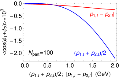
Figure 1: (Color online) The two-particle azimuthal correlation $\left\langle\cos(\phi_{1}+\phi_{2})\right\rangle$ vs $p_{+}=(p_{1,t}+p_{2,t})/2$ (blue line) and $p_{-}=\left|p_{1,t}-p_{2,t}\right|$ (red line) for $N_{part}=100$.

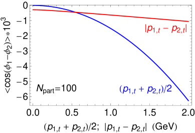
Figure 2: (Color online) The two-particle azimuthal correlation $\left\langle\cos(\phi_{1}-\phi_{2})\right\rangle$ vs $p_{+}=(p_{1,t}+p_{2,t})/2$ (blue line) and $p_{-}=\left|p_{1,t}-p_{2,t}\right|$ (red line) for $N_{part}=100$.

Again, similarly to what has been observed in the STAR data, the correlation $\left\langle\cos(\phi_{1}+\phi_{2})\right\rangle$ grows rapidly with increasing $p_{+}$ while appears much flatter with increasing $p_{-}$. Comparing our results with the STAR data we see that the transverse momentum conservation gives comparable signal for $p_{+}$ and $p_{-}$ larger than $1$ GeV and underestimate the data for lower values of $p_{+}$ and $p_{-}$.

Finally let us discus the pseudorapidity dependence of the correlation $\left\langle\cos(\phi_{1}+\phi_{2})\right\rangle$. The dependence of $\left\langle\cos(\phi_{1}+\phi_{2})\right\rangle$ on $\left|\eta_{1}-\eta_{2}\right|$ has been measured by STAR and found to be dominated by $\left|\eta_{1}-\eta_{2}\right|<2$, which is consistent with the CME expectation. It is quite clear that such dependence cannot be obtained in the present calculation, as no pseudorapidity dependence appears in the nontrivial part of the two-particle correlation function shown in Eq. (11). Consequently, transverse momentum conservation predicts the correlator $\left\langle\cos(\phi_{1}+\phi_{2})\right\rangle$ to be essentially flat as a function of $\left|\eta_{1}-\eta_{2}\right|$ in the midrapidity region except for a very mild dependence due to the slight dependence of $f(\vec{p})$ and $v_{2}$ on $\eta$. However, here we have assumed that the transverse momentum is balanced over the entire rapidity interval. In an actual heavy ion reaction it is not unreasonable to expect that the transverse momentum is balanced over a shorter rapidity interval. If this were the case, we would predict not only a stronger rapidity dependence of the signal but also a considerably stronger signal at midrapidity. Therefore, it would be worthwhile to construct and measure an equivalent of the charge balance function [32] for the transverse momentum. This problem is currently under our consideration.

5 Conclusions and comments

We have quantitatively investigated the contribution of transverse momentum conservation to the azimuthal correlation observables $\gamma=\left\langle\cos(\phi_{1}+\phi_{2})\right\rangle$ and $\delta=\left\langle\cos(\phi_{1}-\phi_{2})\right\rangle$ measured by the STAR collaboration as motivated by the possible strong local parity violation and Chiral Magnetic Effect. Our conclusions can be summarized as follows.

• The contribution due to transverse momentum conservation is comparable in magnitude to the prediction of the Chiral Magnetic Effect as well as the data. In the STAR acceptance we find this contribution to be approximately equal to $\gamma\approx-1.7v_{2}/N$, where $v_{2}$ is the elliptic flow coefficient at midrapidity and $N$ is the total number of produced particles (neutral and charged). This result suggests rather week energy dependence at RHIC since $v_{2}$ and $N$ scale similarly with energy.

• Taking $v_{2}=0.06$ and $N=21N_{part}$ where $N_{part}$ is the number of participants we obtained $\gamma\cdot N_{part}\approx-0.005$, which is a factor $3-5$ (very peripheral – mid-central) smaller than the experimental data. Thus we may conclude that the transverse momentum conservation alone cannot explain the data. Also there is no charge-dependence as opposed to experimental data. It is however a significant source of background that eventually must be quantified and taken into account if one really wants to extract the possible CME from the present (and future) data.

• We have demonstrated that finite acceptance issues, i.e. the facts that particles are measured in a relatively narrow pseudorapidity bin and neutral particles are not detected, do not suppress the effect of transverse momentum conservation on $\gamma$.

• We studied the dependence of $\gamma$ vs $p_{+}=(p_{1,t}+p_{2,t})/2$ and $p_{-}=\left|p_{1,t}-p_{2,t}\right|$. We found that $\gamma$ increases with increasing $p_{+}$, $\gamma\propto(\frac{p_{+}}{\left\langle p_{t}\right\rangle})^{\alpha_{+}}$ with $\alpha_{+}=2-3$. The dependence on $p_{-}$ is much weaker $\gamma\propto(\frac{p_{-}}{\left\langle p_{t}\right\rangle})^{\alpha_{-}}$ with $\alpha_{-}\approx 1$. This behavior is qualitatively similar to what is observed in the data. We also investigated the dependence of $\gamma$ on $|\eta_{1}-\eta_{2}|$ and found no pseudorapidity dependence in contrast to what is observed in the data.

• Finally we calculated $\delta=\left\langle\cos(\phi_{1}-\phi_{2})\right\rangle$ and found that in the STAR acceptance $\delta\approx-1/N$. We found this contribution to be a factor $1.5-4$ (mid-central – very peripheral) larger than the experimental data indicating again that the transverse momentum conservation effect is a significant source of background.

• The present calculation is based on the minimal assumption that the transverse momentum is balanced over all particles (in the full phase space). Thus it is very likely that the calculated contribution to $\gamma$ and $\delta$ from the transverse momentum conservation represents rather the lower limit. Should, as it is not reasonable to assume, the transverse momentum be balanced over a finite rapidity interval, we predict not only a stronger effect at midrapidity but also a rapidity dependence of the correlation function $\gamma$ and $\delta$. Thus a measurement of something like a transverse momentum balance function would be highly desirable. This problem is currently under our consideration.

We end this paper with a few further comments.

• While transverse momentum conservation alone is not sufficient to explaining the data, one may combine it with other effects such as the Chiral Magnetic Effect or Local Charge Conservation [10] to get closer to the data. In Table. 1 we summarize the estimated contributions to the azimuthal correlations from these effects together with the STAR data. All numbers quoted are for $AuAu$ $200$ GeV collisions at about $50-60\%$ centrality (corresponding to $N_{part}\approx 50$ [33]).

  $\hat{O}\times 10^{3}$	$\left\langle\cos(\phi_{1}+\phi_{2})\right\rangle_{++}$	$\left\langle\cos(\phi_{1}+\phi_{2})\right\rangle_{+-}$	$\left\langle\cos(\phi_{1}-\phi_{2})\right\rangle_{++}$	$\left\langle\cos(\phi_{1}-\phi_{2})\right\rangle_{+-}$
  CME	$-(0.1-1)$	$+(0.01-0.1)$	$+(0.1-1)$	$-(0.01-0.1)$
  LCC	$\sim 0$	$+(0.1-1)$	$\sim 0$	$+(1-10)$
  TMC	$\sim-0.1$	$\sim-0.1$	$\sim-1$	$\sim-1$
  DATA	$-0.45$	$+0.06$	$-0.38$	$+1.97$

  Table 1: Estimated contributions to azimuthal correlations from various effects and comparison with data. CME, LCC, and TMC stand for Chiral Magnetic Effect, Local Charge Conservation, and Transverse Momentum Conservation, respectively, while the DATA is from STAR measurement for $AuAu$ $200$ GeV collisions at about $50-60\%$ centrality.

  As a precaution, all numbers (except the STAR data) bear considerable uncertainty. The numbers from Chiral Magnetic Effect (CME) for observables $\left\langle\cos(\phi_{1}+\phi_{2})\right\rangle_{++,+-}$ are extracted from [4]. The numbers for $\left\langle\cos(\phi_{1}-\phi_{2})\right\rangle_{++,+-}$ where obtained using the relation $\left\langle\cos(\phi_{1}-\phi_{2})\right\rangle_{++}=-\left\langle\cos(\phi_{1}+\phi_{2})\right\rangle_{++}$ and analogously for $(+,-)$, which hold in case of a pure CME. The numbers from Local Charge Conservation (LCC) are inferred from [10]: the authors showed the difference $\left\langle\cos(\phi_{1}+\phi_{2})\right\rangle_{+-}-\frac{1}{2}\left[\left\langle\cos(\phi_{1}+\phi_{2})\right\rangle_{++}+\left\langle\cos(\phi_{1}+\phi_{2})\right\rangle_{--}\right]$. From LCC one should expect $\left\langle\cos(\phi_{1}+\phi_{2})\right\rangle_{++,--}\sim 0$ so the $\left\langle\cos(\phi_{1}+\phi_{2})\right\rangle_{+-}$ could be inferred. Furthermore the value for $\left\langle\cos(\phi_{1}-\phi_{2})\right\rangle_{+-}$ is estimated by $\left\langle\cos(\phi_{1}-\phi_{2})\right\rangle_{+-}\sim\left\langle\cos(\phi_{1}+\phi_{2})\right\rangle_{+-}/v_{2}$. Finally as the authors pointed out, their results represent an upper limit of the magnitude for LCC as they enforce exactly local charge neutrality. Our results for Transverse Momentum Conservation (TMC) are as given in the previous sections (with the expected uncertainty within a few tens of percent). The STAR data is from [7]. Even though these are rough estimates, one still can make a few observations: first, no single effect shows a pattern for all observables that are in accord with data; second, different correlators appear to be dominated by different effects, in particular – both CME and TMC provide important contributions to $\left\langle\cos(\phi_{1}+\phi_{2})\right\rangle_{++}$, while TMC seems necessary for explaining the $\left\langle\cos(\phi_{1}-\phi_{2})\right\rangle_{++}$, and LCC for the observed value of $\left\langle\cos(\phi_{1}-\phi_{2})\right\rangle_{+-}$. The situation for $\left\langle\cos(\phi_{1}+\phi_{2})\right\rangle_{+-}$ on the other is more complicated and none of the effects discussed here seems to dominate. Clearly, additional measurements will be required to disentangle this situation.

• As far as comparisons of the data with models is concerned, such as the ones presented by the STAR collaboration [7], one has to ensure that the model satisfies at least two criteria. First, the model has to conserve transverse momentum not only on average but event-by-event. Second, the model has to reproduce the measured magnitude of the elliptic flow, $v_{2}$, as essentially all “trivial” contributions to ${⟨\cos ({\varphi }_1+{\varphi }_{}}_{}$

References

- [1] T. Schafer and E. V. Shuryak, Rev. Mod. Phys. 70, 323 (1998). G. ’t Hooft, arXiv:hep-th/0010225. D. Diakonov, Prog. Part. Nucl. Phys. 51, 173 (2003). G. S. Bali, arXiv:hep-ph/9809351. J. Greensite, Prog. Part. Nucl. Phys. 51, 1 (2003).
- [2] D. J. Gross, R. D. Pisarski and L. G. Yaffe, Rev. Mod. Phys. 53, 43 (1981). L. D. McLerran, E. Mottola and M. E. Shaposhnikov, Phys. Rev. D 43, 2027 (1991). D. Diakonov and V. Petrov, Phys. Rev. D 76, 056001 (2007). J. Liao and E. Shuryak, Phys. Rev. C 75, 054907 (2007); Phys. Rev. Lett. 101, 162302 (2008); Nucl. Phys. A 775, 224 (2006).
- [3] D.E. Kharzeev, R.D. Pisarski and M.H.G. Tytgat, Phys. Rev. Lett. 81, 512 (1998); D.E. Kharzeev and R.D. Pisarski, Phys. Rev. D61, 111901 (2000).
- [4] D.E. Kharzeev, L.D. McLerran and H.J. Warringa, Nucl. Phys. A803, 227 (2008).
- [5] K. Fukushima, D.E. Kharzeev and H.J. Warringa, Phys. Rev. D78, 074033 (2008); Phys. Rev. Lett. 104, 212001 (2010).
- [6] D.E. Kharzeev, Annals Phys. 325, 205 (2010).
- [7] STAR Collaboration, B.I. Abelev et al., Phys. Rev. Lett. 103, 251601 (2009); Phys. Rev. C81, 054908 (2010).
- [8] S.A. Voloshin, Phys. Rev. C 70, 057901 (2004).
- [9] F. Wang, Phys. Rev. C81, 064902 (2010).
- [10] S. Schlichting and S. Pratt, e-Print: arXiv:1005.5341 [nucl-th].
- [11] S. Pratt, e-Print: arXiv:1002.1758 [nucl-th].
- [12] M. Asakawa, A. Majumder and B. Muller, Phys. Rev. C81, 064912 (2010)
- [13] R. Millo and E.V. Shuryak, e-Print: arXiv:0912.4894 [hep-ph].
- [14] A. Bzdak, V. Koch and J. Liao, Phys. Rev. C81, 031901 (2010).
- [15] J. Liao, V. Koch and A. Bzdak, e-Print: arXiv:1005.5380 [nucl-th].
- [16] S. A. Voloshin, arXiv:1006.1020 [nucl-th].
- [17] G. Basar, G.V. Dunne and D.E. Kharzeev, Phys. Rev. Lett. 104, 232301 (2010).
- [18] K. Fukushima, D.E. Kharzeev and H.J. Warringa, Nucl. Phys. A836, 311 (2010).
- [19] Z. B. Kang and D. E. Kharzeev, arXiv:1006.2132 [hep-ph].
- [20] S. A. Voloshin, A. M. Poskanzer and R. Snellings, arXiv:0809.2949 [nucl-ex].
- [21] Z. Chajecki and M. Lisa, Phys. Rev. C78, 064903 (2008); Phys. Rev. C79, 034908 (2009).
- [22] N. Borghini, P.M. Dinh and J.-Y. Ollitrault, Phys. Rev. C62, 034902 (2000).
- [23] STAR Collaboration, J. Adams et al., Phys. Rev. C73, 064907 (2006).
- [24] P. Danielewicz at al., Phys. Rev. C 38, 120 (1988).
- [25] PHOBOS Collaboration, B.B. Back et al., Phys. Rev. C 74, 021901(R) (2006).
- [26] A. Bialas, M. Bleszynski and W. Czyz, Nucl. Phys. B111 (1976) 461.
- [27] BRAHMS Collaboration, I.G. Bearden et al., Phys. Rev. Lett. 94, 162301 (2005).
- [28] PHOBOS Collaboration, B.B. Back et al., Phys. Rev. Lett. 91 (2003) 052303.
- [29] PHOBOS Collaboration, B.B. Back et al., Phys. Rev. C72, 051901(R) (2005); B. Alver et al., Phys. Rev. Lett. 98, 242302 (2007).
- [30] STAR Collaboration, K.H. Ackermann et al., Phys. Rev. Lett. 86 (2001) 402; J. Adams et al., Phys. Rev. C72 (2005) 014904.
- [31] PHENIX Collaboration, S.S. Adler et al., Phys. Rev. Lett. 91 (2003) 182301; S. Afanasiev et al., Phys. Rev. C80 (2009) 024909.
- [32] S.A. Bass, P. Danielewicz and S. Pratt, Phys. Rev. Lett. 85 (2000) 2689.
- [33] STAR Collaboration, B.I. Abelev et al., Phys. Rev. C79 (2009) 034909.
- [34] M. Bleicher and H. Stoecker, Phys. Lett. B526 (2002) 309; X. Zhu, M. Bleicher and H. Stoecker, Phys. Rev. C72 (2005) 064911.