Abstract

Motivated by its relation to the Pohlmeyer reduction of $AdS_{5}\times S^{5}$ superstring theory we continue the investigation of the generalized sine-Gordon model defined by $SO(N+1)/SO(N)$ gauged WZW theory with an integrable potential. Extending our previous work (arXiv:0912.2958) we compute the one-loop two-particle S-matrix for the elementary massive excitations. In the $N=2$ case corresponding to the complex sine-Gordon theory it agrees with the charge-one sector of the quantum soliton S-matrix proposed in hep-th/9410140. In the case of $N>2$ when the gauge group $SO(N)$ is non-abelian we find a curious anomaly in the Yang-Baxter equation which we interpret as a gauge artifact related to the fact that the scattered particles are not singlets under the residual global subgroup of the gauge group.

1 Introduction

In this paper we continue the investigation [2] of the perturbative S-matrix of generalised sine-Gordon models. Various examples of such models (called also “symmetric space sine-Gordon models”) based on a $G/H$ gauged WZW model with an integrable potential term were considered in, e.g., [3, 4, 5, 6, 7].

The action for these $G/H$ models is given by the (asymmetrically) gauged WZW action with a potential term,

$$\begin{split}\mathcal{S}&=-\ \frac{k}{8\pi\nu}\textrm{Tr}\Big{[}\frac{1}{2}\,\int d^{2}x\;\ g^{-1}\partial_{+}g\ g^{-1}\partial_{-}g\ -\frac{1}{3}\,\int d^{3}x\;\ \epsilon^{mnl}\ g^{-1}\partial_{m}g\ g^{-1}\partial_{n}g\ g^{-1}\partial_{l}g\\ &\qquad\quad+\,\int d^{2}x\;\ \big{(}A_{+}\partial_{-}gg^{-1}-A_{-}g^{-1}\partial_{+}g-g^{-1}A_{+}gA_{-}+\tau(A_{+})A_{-}\big{)}\\ &\qquad\quad+m^{2}\,\int d^{2}x\;\ (g^{-1}TgT-T^{2})\Big{]}\,.\end{split}$$ (1.1)

Here $g\in G$, $A_{\pm}\in\mathfrak{h}$=alg$(H)$, $k$ is a level and $m$ is a parameter defining the mass of elementary excitations near $g=1$. The standard symmetric gauging corresponds to $\tau=\textbf{1}$ ($\tau$ is an automorphism of $\mathfrak{h}$); for an abelian gauge group $H$ there is an option of axial gauging corresponding to $\tau(h)=-h$. The constant matrix $T$ defining the potential is chosen to commute with $H$ (see, e.g., [8, 9] for details).

Recent interest in such models is due to their relation, via the Pohlmeyer reduction, to classical string theory on symmetric spaces [3, 10, 11, 8, 12, 9, 13, 14]. In the case of the $AdS_{5}\times S^{5}$ superstring theory the classical Pohlmeyer reduction leads to a special integrable massive 2d theory defined by the $G/H=[SO(1,4)\times SO(5)]/[SO(4)\times SO(4)]$ gauged WZW model with an integrable potential and coupled to a particular set of 2d fermions [8, 15]. The corresponding quantum theory has certain unique features (it is UV finite [16] and is closely related to the original $AdS_{5}\times S^{5}$ superstring at the one-loop level [17, 18]). This suggests [8] that it may, in fact, be quantum-equivalent to the $AdS_{5}\times S^{5}$ superstring. If that were indeed the case, this theory could be used as a starting point for a 2-d Lorentz covariant “first-principles” solution of the $AdS_{5}\times S^{5}$ superstring based on finding an exact soliton S-matrix, just as in the case of standard 2d sigma models [19] or for some similar massive theories [20, 14] (see also [21]).

An important check of a proposal for an exact quantum soliton S-matrix of an integrable theory would be to demonstrate its consistency with the perturbative S-matrix computed from the path integral defined by the classical action.

This motivates the study of perturbative S-matrices of such generalized sine-Gordon models with a non-abelian gauge symmetry $H$. In [2] we computed the tree-level two-particle S-matrix for the bosonic $SO(N+1)/SO(N)$ theory and then for the full reduced theory associated to the $AdS_{5}\times S^{5}$ superstring. The resulting S-matrix exhibited some remarkable features, in particular, it group-factorised in the same way as the non Lorentz invariant tree-level $\mathfrak{psu}(2|2)\oplus\mathfrak{psu}(2|2)$ invariant light-cone gauge S-matrix [22] of the $AdS_{5}\times S^{5}$ superstring. It also had an intriguing similarity with the classical $\mathfrak{psu}(2|2)$ trigonometric r-matrix of [23, 24].

The next important step towards unravelling the full structure of the S-matrix of the reduced theory is to extend the tree-level computation of [2] to the one-loop level. In this paper we address this problem for the bosonic $SO(N+1)/SO(N)$ theory, hoping to return to the complete $[SO(1,4)\times SO(5)]/[SO(4)\times SO(4)]$ theory with fermions in the future.

There are technical issues involved in computing the perturbative S-matrix for the generalised sine-Gordon theories defined by (1.1). Such models were mostly studied for abelian gauge groups $H$ [7, 25, 26, 27, 28], of which the complex sine-Gordon model is a prime example. In this case there is an option of axial gauging, in which case the vacuum is unique up to gauge transformations. In the case of a non-abelian $H$ there is a non-trivial vacuum moduli space, no global symmetry and on integrating out the gauge fields $A_{\pm}$ one is left with a Lagrangian that has no perturbative expansion about the trivial vacuum. As was argued in [2], the problem with expansion is an artifact of the gauge fixing procedure on $g$. If instead one chooses the “light-cone” gauge $A_{+}=0$ [2] one is able to construct a perturbative Lagrangian for the asymptotic excitations and thus compute the tree-level S-matrix. Going beyond tree level requires, however, taking into account the non-trivial contribution of the delta-function constraint resulting from integrating over $A_{-}$ in the path integral for the action (1.1).

Below we will start with the case of the $SU(2)/U(1)$ axially gauged theory corresponding to the complex sine-Gordon (CsG) model. The tree-level S-matrix of this theory [29] satisfies the Yang-Baxter equation. The Yang-Baxter equation, however, is violated at the one-loop level for the “naive” S-matrix obtained directly from the standard CsG action, following from (1.1) upon solving for $A_{\pm}$. The quantum theory based on this CsG action was studied in [29, 30, 31] where it was suggested to add a quantum counterterm to restore factorised scattering. In reference [20] the exact quantum soliton S-matrix satisfying the Yang-Baxter equation was proposed. It was conjectured that if the quantum CsG model is defined in terms of the $SU(2)/U(1)$ gauged WZW theory (1.1) then the necessary quantum counterterms required to obtain a factorizable perturbative S-matrix consistent with the exact S-matrix should appear automatically.

We will demonstrate that this is indeed the case at the one-loop level. We will show that equivalent “counterterms” (leading to the same S-matrix) can be obtained (i) from the quantum effective action of the gauged WZW model [32], or (ii) directly from the determinant resulting from integrating out the non-dynamical fields $(A_{+},A_{-})$, or (iii) from the delta-function constraint in the $A_{+}=0$ gauge.

We will then extend the $A_{+}=0$ gauge approach to the general $SO(N+1)/SO(N)$ theory. In the case of the non-abelian gauge group $H=SO(N)$ the resulting S-matrix will be found to violate the standard Yang-Baxter equation already at the tree level, but we will suggest that this should not contradict the quantum integrability of the theory being a gauge artifact (the excitations we scatter transform non-trivially under unbroken global part of the gauge group).

Further clarification of this issue and the extension to the full reduced theory for the $AdS_{5}\times S^{5}$ superstring are among the important problems for the future.

The structure of the rest of this paper is as follows. In section 2 we review the $A_{+}=0$ gauge approach used to compute the tree-level S-matrix in [2]. We show that fixing this gauge and integrating out the unphysical degrees of freedom gives rise to a functional determinant in the path integral, which leads to a non-trivial contribution to the one-loop S-matrix.

In section 3 we discuss the case of the $SU(2)/U(1)$ theory related to the complex sine-Gordon model. We compute the corresponding one-loop S-matrix using three different methods, one of which uses the $A_{+}=0$ gauge. They all give the same result, equal to the sum of the “naive” one-loop S-matrix of [29] with a non-trivial correction. The total one-loop S-matrix matches the expansion of the (charge-one sector of) the quantum soliton S-matrix of [20].

In section 4 we generalise the computation of the one-loop S-matrix in the $A_{+}=0$ gauge to the non-abelian $G/H=SO(N+1)/SO(N)$ theory. The resulting S-matrix turns out to violate the standard Yang-Baxter equation in the case of non-abelian gauge symmetry. We discuss the remarkably simple structure of this violation at the tree level and possible ways to resolve an apparent contradiction with the expected quantum integrability of the underlying theory.

The appendix contains a demonstration of a relation between two effective Lagrangians used to compute the one-loop complex sine-Gordon S-matrix in section 3.

2 Gauged WZW theory with an integrable potential
in the gauge $A_{+}=0$

In this section we shall start by reviewing the result of [2] for the tree-level S-matrix of the massive excitations of the gauged WZW action with an integrable potential, (1.1). We will then generalise the computation of the S-matrix to the one-loop order.

As in [2] we assume that $G$ is a compact group and that the corresponding algebra $\mathfrak{g}$ admits an orthogonal decomposition

$$\mathfrak{g}=\mathfrak{h}\oplus\mathfrak{m}\,,$$ (2.1)

where $\mathfrak{h}$ is the algebra corresponding to the gauge group $H$, and $\mathfrak{m}$ is the orthogonal complement of $\mathfrak{h}$ in $\mathfrak{g}$. We also assume that $G/H$ is a symmetric coset space, i.e.

$$\begin{array}[]{ccc}[\mathfrak{h},\,\mathfrak{h}]\subset\mathfrak{h}\,,&[\mathfrak{h},\,\mathfrak{m}]\subset\mathfrak{m}\,,&[\mathfrak{m},\,\mathfrak{m}]\subset\mathfrak{h}\,,\\ &\textrm{Tr}(\mathfrak{m}\,\mathfrak{h})=0\,,&\end{array}$$ (2.2)

and that we have an orthogonal basis of a matrix representation of $\mathfrak{g}$, the elements of which we denote as follows

• ${\rm T}_{i}$, where $i=\dim\mathfrak{m}+1,\ldots,\,\dim\mathfrak{g}$   is a basis for $\mathfrak{h}$;

• ${\rm T}_{a}$, where $a=1,\ldots,\,\dim\mathfrak{m}$   is a basis for $\mathfrak{m}$;

• ${\rm T}_{A}=\{{\rm T}_{a},{\rm T}_{i}\}$, where $A=1,\ldots,\,\dim\mathfrak{g}$   is an orthogonal basis for $\mathfrak{g}$, that is

  $$\textrm{Tr}({\rm T}_{A}{\rm T}_{B})=-K^{2}\delta_{AB}\,.$$ (2.3)

$K$ is a constant that will be fixed so that the quadratic kinetic terms in the action have canonical form. $K$ will depend on the coupling $k$, in particular, $K\sim k^{-\frac{1}{2}}$.

The structure constants of the algebra $\mathfrak{g}$ are defined by

$$[{\rm T}_{A},\,{\rm T}_{B}]=f_{ABC}{\rm T}_{C}\,,$$ (2.4)

with $f_{ABC}$ being completely antisymmetric. From the commutation relations (2.2) we have $f_{aij}=f_{abc}=0$. Due to the normalization of the generators in (2.3) the structure constants will also have the coupling dependence, $f_{ABC}\sim k^{-\frac{1}{2}}$.

As in [2], we shall fix the gauge $A_{+}=0$ in the path integral defined by the action $\mathcal{S}[g,A_{+},A_{-}]$ in (1.1) and integrate out $A_{-}$, getting

$$\mathcal{Z}=\int[dg]\;\;\delta\big{[}(g^{-1}\partial_{+}g)|_{\mathfrak{h}}\big{]}\;\;e^{i\mathcal{S}[g,0,0]}\,.$$ (2.5)

The gauge $A_{+}=0$ preserves the Lorentz invariance in 2 dimensions but like the analogous light-cone gauge in Yang-Mills theory it does not fix the global part of the gauge group $H$.

2.1 Expansion of the gauge-fixed action

To compute the S-matrix we will need to expand the action, (1.1), near a trivial vacuum $g=1$ and solve the delta-function constraint in (2.5). Following [2], we parametrise $g$ as follows

$$g=e^{\eta}\,,\hskip 30.0pt\eta\in\mathfrak{g}\,,$$ (2.6)

and expand in $\eta$, ^,

$$\!\!\,\,\,\mathcal{S}[g(\eta),0,0]=-\frac{1}{8\pi\nu}\ \int d^{2}x\;\ \textrm{Tr}\Big{(}\sum_{n=0}^{\infty}\frac{k}{(n+2)!}\big{[}\;\partial_{+}\eta\,\mathfrak{L}^{\;n}_{\eta}(\partial_{-}\eta)-m^{2}\;\mathfrak{L}_{\eta}(T)\,\mathfrak{L}^{\;n+1}(T)\big{]}\Big{)}\,.$$ (2.7)

Using the orthogonal decomposition of $\mathfrak{g}$, (2.1), we split $\eta$ as

$$\eta=X+\xi\,,\hskip 30.0ptX\in\mathfrak{m}\,,\hskip 10.0pt\xi\in\mathfrak{h}\,.$$ (2.8)

The coset component $X$ represents $\dim\,\mathfrak{m}$ massive asymptotic excitations (as seen by solving the gauge-fixed linearised equations of motion), for which the tree-level two-particle S-matrix was found in [2]. Here we will compute the one-loop correction to their perturbative S-matrix.

At the classical level we can use the $\delta$-function constraint in (2.5) to solve for the “gauge component” $\xi$ in terms of $X$. Expanding $\big{(}g^{-1}\partial_{+}g\big{)}\big{|}_{\mathfrak{h}}=0$ to cubic order in fields we get

$$\begin{split}\partial_{+}\xi&-\frac{1}{2}[X,\,\partial_{+}X]-\frac{1}{2}[\xi,\,\partial_{+}\xi]\\ &+\frac{1}{6}[X,\,[X,\,\partial_{+}\xi]]+\frac{1}{6}[X,\,[\xi,\,\partial_{+}X]]+\frac{1}{6}[\xi,\,[X,\,\partial_{+}X]]+\frac{1}{6}[\xi,\,[\xi,\,\partial_{+}\xi]]+\ldots=0\,.\end{split}$$ (2.9)

Solving perturbatively for $\xi$ gives

$$\xi_{0}[X]=\frac{1}{2}\frac{1}{\partial_{+}}[X,\,\partial_{+}X]+\mathcal{O}(X^{4})\,.$$ (2.10)

As $\xi_{0}[X]\sim{X^{2}}$, when $\xi=\xi_{0}[X]$ is substituted into the action there will be no cubic terms in $X$. Thus, to compute the one-loop S-matrix, we only need the part of the action which is of quartic order in $X$. Substituting (2.8) and (2.10) into (2.7), using integration by parts and the Jacobi identity, we end up with the following remarkably simple local action [2],

$$\mathcal{S}[g(\eta(X,\xi_{0}[X])),0,0] \!\!\!= \!\!\!-\frac{k}{8\pi\nu}\int d^{2}x\;\textrm{Tr}\Big{[}\,\frac{1}{2}\partial_{+}X\partial_{-}X-\frac{m^{2}}{2}[X,\,T][X,\,T]$$

$$\hskip 15.0pt+\ \frac{1}{12}[X,\,\partial_{+}X][X,\,\partial_{-}X]+\frac{m^{2}}{24}[X,\,[X,\,T]][X,\,[X,\,T]]+\mathcal{O}(X^{6})\Big{]}\,.$$

This action can be used to compute the tree-level two-particle S-matrix [2], as well as the part of the one-loop two-particle S-matrix given by bubble diagrams. The only additional piece of information one needs to know is the commutation relations with the matrix $T$ in the potential, which depend on the particular choice of the groups $G$ and $H$. The calculations then reduce to standard Feynman integrals.

Let us note that the renormalization of the general theory (1.1) was discussed in [16]. The WZW coupling $k$ is not, of course, renormalized but there is a logarithmic UV renormalization of the mass parameter $m^{2}$ (as well as a field renormalization). One may choose a scheme ($\overline{\rm MS}$ scheme) in which there is no finite renormalization of $m^{2}$ at the one-loop order. This will be assumed below.

The aim of the rest of this section will be to discuss the non-trivial contribution of the path integral constraint in (2.5) to the one-loop S-matrix. Thus we will not present the detailed expressions for the S-matrix terms arising from the Lagrangian. The explicit results will be given for the particular cases of $G/H=SU(2)/U(1)$ and $G/H=SO(N+1)/SO(N)$ in later sections.

2.2 Functional determinant contribution

At the quantum level, solving the delta-function constraint (2.9) to eliminate $\xi$ from the path integral (2.5) will give rise to a field-dependent functional determinant. To find it we functionally differentiate the constraint equation (2.9) and evalute the resulting operator on $\xi=\xi_{0}[X]$ in (2.10). The resulting contribution to the path integral is then given by

$$\big{(}\det\mathcal{Q}\big{)}^{-1}\ ,$$ (2.12)

$$\mathcal{Q}\zeta=\partial_{+}\zeta-\frac{1}{4}[\frac{1}{\partial_{+}}[X,\,\partial_{+}X],\,\partial_{+}\zeta]+\frac{1}{4}[[X,\,\partial_{+}X],\,\zeta]$$ (2.13)

$$\hskip 50.0pt+\ \frac{1}{6}[X,\,[X,\,\partial_{+}\zeta]]-\frac{1}{6}[X,\,[\partial_{+}X,\,\zeta]]-\frac{1}{6}[[X,\,\partial_{+}X],\,\zeta]+\mathcal{O}(X^{4})\,,$$ (2.14)

where the operator $\mathcal{Q}$ acts on a function $\zeta$ taking values in $\mathfrak{h}$.

Let us rewrite the operator $\mathcal{Q}$ in the following form

$$\mathcal{Q}=\vec{\partial_{+}}(1+\alpha[X])+\beta[X]\,,$$ (2.15)

where the $\;\,\vec{}\;\,$ symbol denotes the operator acting all the way to the right. $\alpha$ and $\beta$ are functions of $X$ and $\partial X$ that are both $\mathcal{O}(X^{2})$.

The prescription we shall use is to expand the determinant of $\mathcal{Q}$ (2.15) in the usual perturbative way, treating $\vec{\partial_{+}}$ as the free part. We shall ignore all quadratic divergences and tadpole contributions. Then to evaluate the contribution of the determinant to the two-particle one-loop S-matrix we may ignore $\alpha[X]$ and $\beta_{n}[X]$ for $n\geq 4$. Factorising out the free part of the operator, we have

$$\ln(\det[\partial_{+}^{-1}\mathcal{Q}])^{-1}=-\textrm{tr}\ln[\partial_{+}^{-1}\mathcal{Q}]\,.$$ (2.16)

One may then extract the $\mathcal{O}(X^{4})$ part,

$$-\textrm{tr}\big{(}\alpha_{4}[X]+\partial_{+}^{-1}\beta_{4}[X]\big{)}-\frac{1}{2}\textrm{tr}\big{(}\alpha_{2}[X]+\partial_{+}^{-1}\beta_{2}[X]\big{)}^{2}\,.$$ (2.17)

The traces of $\alpha_{4}[X]$ in the first term and of $\alpha_{2}[X]^{2}$ in the second term both give quadratic divergences, which we ignore. The trace of $\partial_{+}^{-1}\beta_{4}[X]$ in the first term and the cross-terms in the second term both give tadpole integrals which we also set to zero. We are then left with

$$-\textrm{tr}\big{(}\partial_{+}^{-1}\beta_{2}[X]\big{)}^{2}\,$$ (2.18)

from the second term in (2.17).

Let us note that moving the free operator $\vec{\partial_{+}}$ all the way to the left and setting tadpoles to vanish can be reinterpreted as choosing a different parametrisation of $g$. For example, we may choose instead of (2.6),(2.8) the following parametrisation

$$g=e^{\eta}\,,\hskip 20.0pt\eta=X+\xi-\alpha_{2}[X]\xi\,.$$ (2.19)

The operator (2.15) would be corrected to $\mathcal{O}(X^{2})$ as follows

$$\mathcal{Q}=\vec{\partial_{+}}(1+\alpha[X])+\beta[X]-\vec{\partial_{+}}\alpha_{2}[X]+\mathcal{O}(X^{4})=\vec{\partial_{+}}+\beta_{2}[X]+\mathcal{O}(X^{4})\,,$$ (2.20)

i.e. the $\mathcal{O}(X^{2})$ part of $\alpha[X]$ will cancel. Thus the prescription detailed above can be seen to be equivalent to a field redefinition of $\xi$ by some function of $X$ and $\partial X$ or choosing an alternative measure for $\xi$ in the path integral.

As we shall see below, in the complex sine-Gordon case computing the determinant contribution with this prescription will give corrections to the S-matrix that match the results found using two alternative methods described in sections 3.3.1 and 3.3.2 and also match the soliton S-matrix of [20].

Next, let us expand $X$ in generators

$$X=X_{a}{\rm T}_{a}\,,$$ (2.21)

and use the Jacobi identity to rewrite the determinant (2.12) of (2.15) in the form

$$\begin{split}-\textrm{tr}\ln\bigg{[}\vec{\partial_{+}}&\Big{(}\delta_{ij}-\frac{1}{4}\frac{1}{\partial_{+}}(X_{a}\partial_{+}X_{b})f_{abk}f_{ijk}-\frac{1}{6}X_{a}X_{b}f_{aci}f_{bcj}\Big{)}\\ &\hskip 100.0pt+\frac{1}{2}X_{a}\partial_{+}X_{b}f_{aic}f_{bjc}+\mathcal{O}(X^{-4})\bigg{]}\,.\end{split}$$ (2.22)

Following the above prescription, let us now ignore the term corresponding to $\alpha[X]$ in (2.15), getting

$$\begin{split}-\textrm{tr}\ln\big{(}\delta_{ij}\partial_{+}+\frac{1}{2}V_{abij}X_{a}\partial_{+}X_{b}\big{)}\,,\ \ \ \ \ \ \ \ \ \ \ \ \ \ V_{abij}\equiv f_{aic}f_{bjc}\ .\end{split}$$ (2.23)

We may then follow the standard perturbative approach using the Feynman rules in figure 1, that come from (2.23) to compute the Feynman diagrams in figure 2.

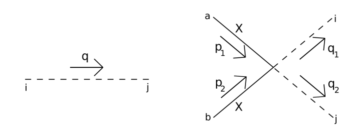
$$\hskip 110.0pt\frac{i\delta_{ij}}{q_{+}}\,,\hskip 95.0pt\frac{i}{2}\Big{[}(p_{1+}+p_{2+})V_{(ab)ij}-(p_{1+}-p_{2+})V_{[ab]ij}\Big{]}\,.$$

Figure 1: Feynman rules

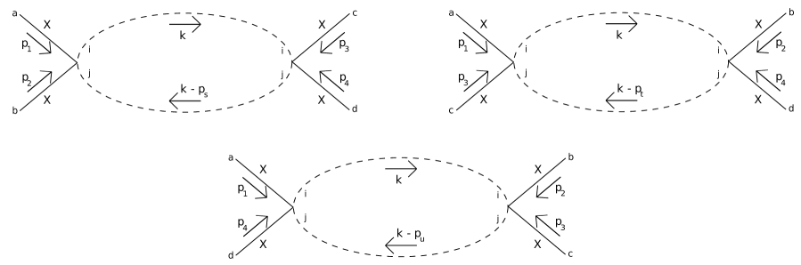
Figure 2: One-loop Feynman diagrams

After solving the momentum conservation constraint and the on-shell condition with

$$p_{1}=-p_{3}=me^{\theta_{1}}\,,\hskip 30.0ptp_{2}=-p_{4}=me^{\theta_{2}}\,,$$ (2.24)

we have

$$\begin{array}[]{cc}\theta\equiv\theta_{1}-\theta_{2}\ ,\\ -p_{s}^{2}=p_{s+}p_{s-}=4m^{2}\cosh^{2}\frac{\theta}{2}\,,\ \ \ \ \ \ \ \ \ p_{s}=p_{1}+p_{2}\,,\\ \ \ \ \ \ \ -p_{t}^{2}=p_{t+}p_{t-}=0\,,\ \ \ \ \ \ \ \ \ \ \ \ \ \ \ \ \ p_{t}=p_{1}+p_{3},\\ -p_{u}^{2}=p_{u+}p_{u-}=4m^{2}\sinh^{2}\frac{\theta}{2}\,,\ \ \ \ \ \ \ \ \ p_{u}=p_{1}+p_{4}\,.\end{array}$$ (2.25)

Given that

$$V_{(ab)ij}V_{[cd]ji}=0\,,$$ (2.26)

and using the standard integral (see, e.g., [33])

$$\int\frac{d^{2}q}{(2\pi)^{2}}\;\frac{1}{q_{+}(q_{+}-p_{+})}=\frac{i}{4\pi}\frac{p_{-}}{p_{+}}\ ,$$ (2.27)

the contributions of the $s,t,u$-channel diagrams in figure 2 to the one-loop S-matrix are found to be respectively

$$\begin{split}\Delta S_{1}=-\frac{i}{16\pi\sinh\theta}&\Big{(}\cosh^{2}\frac{\theta}{2}\ V_{(ab)ij}V_{(cd)ji}+\sinh^{2}\frac{\theta}{2}\ V_{[ab]ij}V_{[cd]ji}\Big{)}\,,\\ \Delta S_{2}=-\frac{i}{16\pi\sinh\theta}&\Big{(}\cosh\theta\ V_{[ac]ij}V_{[bd]ji}\Big{)}\,,\\ \Delta S_{3}=\hskip 8.0pt\frac{i}{16\pi\sinh\theta}&\Big{(}\sinh^{2}\frac{\theta}{2}\ V_{(ad)ij}V_{(bc)ji}-\cosh^{2}\frac{\theta}{2}\ V_{[ad]ij}V_{[bc]ji}\Big{)}\,.\end{split}$$ (2.28)

Here we have included the usual Jacobian factor $\frac{1}{4m^{2}\sinh\theta}$ arising from solving the momentum conservation constraint.

Note that the second of these contributions is somewhat ambiguous when taking the limit $p_{t}\rightarrow 0$. Consider the integral

$$\begin{split}&(p_{1+}-p_{3+})(p_{2+}-p_{4+})\int\frac{d^{2}q}{(2\pi)^{2}}\frac{1}{q_{+}(q_{+}-p_{t+})}=\frac{i}{4\pi}(p_{1+}-p_{3+})(p_{2+}-p_{4+})\frac{p_{t-}}{p_{t+}}\\ =&-\frac{i}{4\pi}(p_{1+}-p_{3+})(p_{4+}-p_{2+})\bigg{(}\frac{p_{1-}+p_{3-}}{p_{1+}+p_{3+}}\bigg{)}^{x}\bigg{(}\frac{p_{2-}+p_{4-}}{p_{2+}+p_{4+}}\bigg{)}^{1-x}\,,\end{split}$$ (2.29)

where we have used that $p_{t}=p_{1}+p_{3}=-(p_{2}+p_{4})$ and introduced an arbitrary parameter $x$. Substituting in for the on-shell momenta in terms of the rapidities $p_{i\pm}=me^{\pm\theta_{i}}\,,$ and taking the limits $\theta_{3}\rightarrow i\pi+\theta_{1},\ \ \theta_{4}\rightarrow i\pi+\theta_{2}\,,$ to solve $p_{t}=0$, we find that the integral (2.29) is

$$\begin{split}&\frac{im^{2}}{\pi}e^{(1-2x)\theta}\,,\end{split}$$ (2.30)

and thus depends on the arbitrary parameter $x$. We may fix this ambiguity by demanding that the resulting S-matrix should satisfy the physical requirements of crossing symmetry and unitarity. Noting that the integral in (2.29) appears in the S-matrix with the factor of $V_{[ac]ij}V_{[bd]ji}$ it is clear that we should take the average of two terms of the type (2.30), one with $x=1$ and one with $x=-1$. This then gives a consistent expression proportional to $\cosh\theta$ presented in (2.28).

3 Complex sine-Gordon model

In this section we will review some relevant aspects of the complex sine-Gordon model (CsG), which at the classical level may be defined as a special 2-d sigma model with a particular integrable potential containing two real bosonic scalar fields and having global $SO(2)$ symmetry  ($a,b,=1,2$)

$$\mathcal{L}=\frac{1}{2}\Big{(}\frac{\partial_{+}\psi_{a}\partial_{-}\psi_{a}}{1-{\rm g}^{2}\psi_{b}\psi_{b}}-m^{2}\psi_{a}\psi_{a}\Big{)}\,,$$ (3.1)

where ${\rm g}$ is a dimensionless coupling and $m$ is the free mass of the elementary excitations.

We shall first recall the perturbative analysis of [29] where it was noticed that the scattering factorisation property is broken at one loop, but may be restored by the addition of quantum counterterms. We shall then discuss the soliton S-matrix of [20], and its relation to the scattering of elementary excitations. In [20] it was suggested that the theory that is quantum-integrable is actually the $SU(2)/U(1)$ gauged WZW model with an integrable potential (1.1). This theory, which reduces to the complex sine-Gordon action of [29] at the classical level, should then be viewed as the proper quantum definition of the latter.

We shall then show how to construct the one-loop counterterms required to preserve the integrability directly from this gauged WZW model, thus providing convincing evidence for the correctness of the proposal of [20].

3.1 Perturbative S-matrix

Following [29] we shall compute the perturbative S-matrix of CsG model, splitting the Lagrangian (3.1) into free and interacting parts

$$\mathcal{L}=-\frac{1}{2}\partial_{+}\psi_{a}\partial_{-}\psi_{a}-\frac{m^{2}}{2}\psi_{a}\psi_{a}+\frac{{\rm g}^{2}}{2}\psi_{b}\psi_{b}\partial_{+}\psi_{a}\partial_{-}\psi_{a}+\mathcal{O}({\rm g}^{4})\,.$$ (3.2)

The S-matrix can be written terms of the three functions $S_{1}(\theta)$, $S_{2}(\theta)$, $S_{3}(\theta)$,

$$\left<\psi_{c}(-p_{3})\psi_{d}(-p_{4})\right|\mathbb{S}\left|\psi_{a}(p_{1})\psi_{b}(p_{2})\right>=(2\pi)^{2}4\epsilon_{p_{1}}\epsilon_{p_{2}}\delta(p_{1}+p_{3})\delta(p_{2}+p_{4})\ S_{ab,cd}(\theta)\,,$$ (3.3)

$$S_{ab,cd}=S_{1}(\theta)\ \delta_{ab}\delta_{cd}+\ S_{2}(\theta)\ \delta_{ac}\delta_{bd}+\ S_{3}(\theta)\ \delta_{ad}\delta_{bc}\,,$$ (3.4)

where $\mathbb{S}$ is the usual scattering operator and $\epsilon_{p}=\sqrt{p^{2}+m^{2}}$ is the on-shell energy associated with the spatial momentum $p$. $\theta$ is the difference of the rapidities of the two on-shell massive particles. The S-matrix is restricted to take this form by the Lorentz and global $SO(2)$ symmetries. Crossing symmetry also implies the following relations,

$$S_{1}(\theta)=S_{3}(i\pi-\theta)\,,\hskip 30.0ptS_{2}(\theta)=S_{2}(i\pi-\theta)\,.$$ (3.5)

In [29] this S-matrix was computed to one-loop order with the result

$$\begin{split}S_{1}(\theta)=&-i{\rm g}^{2}\coth\theta+i\frac{{\rm g}^{4}}{2\pi}(\textrm{\,cosech\,}\theta+\coth\theta)+{\rm g}^{4}\coth\theta\ \textrm{\,cosech\,}\theta+\mathcal{O}({\rm g}^{6})\,,\\ S_{2}(\theta)=&1+i{\rm g}^{2}\textrm{\,cosech\,}\theta-{\rm g}^{4}(\frac{1}{2}+\textrm{\,cosech\,}^{2}\theta)+\mathcal{O}({\rm g}^{6})\,,\\ S_{3}(\theta)=&i{\rm g}^{2}\coth\theta+i\frac{{\rm g}^{4}}{2\pi}(\textrm{\,cosech\,}\theta-\coth\theta)-{\rm g}^{4}\coth\theta\ \textrm{\,cosech\,}\theta+\mathcal{O}({\rm g}^{6})\,.\end{split}$$ (3.6)

Factorised scattering and thus integrability of a 2d theory implies, in general, that the Yang-Baxter equation is satisfied. In the abelian case like the CsG theory of an $SO(2)$ doublet this condition can be reduced to the reflectionless scattering condition, i.e. to the vanishing of the reflection coefficient

$$R(\theta)\equiv S_{1}(\theta)+S_{3}(\theta)=0\,.$$ (3.7)

We can immediately see that while this property is true at the tree level (i.e. to order ${\rm g}^{2}$), it breaks down at one-loop order: we find from (3.6)

$$R(\theta)=\frac{i{\rm g}^{4}}{\pi}\textrm{\,cosech\,}\theta+\mathcal{O}({\rm g}^{6})\,.$$ (3.8)

In [29] it was suggested to add a quantum counterterm to restore the factorised scattering at one-loop order. If such counterterm is required to be ultra-local (no derivatives) then it is found to be unique

$$\Delta\mathcal{L}=\frac{m^{2}{\rm g}^{4}}{4\pi}\psi_{a}\psi_{a}\psi_{b}\psi_{b}\,.$$ (3.9)

Adding its contribution leads to the following “corrected” S-matrix

$$\hat{S}=S+\Delta S\,,$$ (3.10)

$$\begin{split}\hat{S}_{1}(\theta)=&-i{\rm g}^{2}\coth\theta+i\frac{{\rm g}^{4}}{2\pi}\coth\theta+{\rm g}^{4}\coth\theta\ \textrm{\,cosech\,}\theta+\mathcal{O}({\rm g}^{6})\,,\\ \hat{S}_{2}(\theta)=&1+i{\rm g}^{2}\textrm{\,cosech\,}\theta-i\frac{{\rm g}^{4}}{2\pi}\textrm{\,cosech\,}\theta-{\rm g}^{4}(\frac{1}{2}+\textrm{\,cosech\,}^{2}\theta)+\mathcal{O}({\rm g}^{6})\,,\\ \hat{S}_{3}(\theta)=&i{\rm g}^{2}\coth\theta-i\frac{{\rm g}^{4}}{2\pi}\coth\theta-{\rm g}^{4}\coth\theta\ \textrm{\,cosech\,}\theta+\mathcal{O}({\rm g}^{6})\,,\end{split}$$ (3.11)

satisfying the factorisation (or reflectionless (3.7)) property. The authors of [29, 30] conjectured that such counterterm addition procedure should apply to all orders, leading to a factorizable quantum S-matrix.

Let us mention that while in [29] the counterterm was restricted to be ultra-local, this is not, in fact, a necessary requirement: the only condition is that the resulting S-matrix should be reflectionless (or satisfy the Yang-Baxter equation) at the quantum level. For example, one may consider local counterterms with up to two derivatives that may be interpreted as corrections to the sigma model part of the action. This will be relevant below in the context of the gauged WZW theory interpretation of this model.

As implied by the name of the complex sine-Gordon model, it can be interpreted as a theory for a single complex scalar field $Z$

$$Z=\frac{1}{\sqrt{2}}(\psi_{1}+i\psi_{2})\,.$$ (3.12)

Using the global $U(1)$ and the 2d Lorentz symmetry the scattering matrix may be represented in the complex $Z$ basis as

$$\begin{split}\mathbb{S}\left|Z(p_{1})Z(p_{2})\right>=&S_{++++}(\theta)\left|Z(p_{1})Z(p_{2})\right>\,,\\ \mathbb{S}\left|Z(p_{1})Z^{*}(p_{2})\right>=&S_{+-+-}(\theta)\left|Z(p_{1})Z^{*}(p_{2})\right>+S_{+--+}(\theta)\left|Z^{*}(p_{1})Z_{(}p_{2})\right>\,,\\ \mathbb{S}\left|Z^{*}(p_{1})Z^{*}(p_{2})\right>=&S_{----}(\theta)\left|Z^{*}(p_{1})Z^{*}(p_{2})\right>\,,\end{split}$$ (3.13)

where in terms of the functions in (3.4) we have

$$\begin{array}[]{c}S_{++++}(\theta)=S_{----}(\theta)=S_{2}(\theta)+S_{3}(\theta)\,,\\ S_{+-+-}(\theta)=S_{1}(\theta)+S_{2}(\theta)\,,\hskip 20.0ptS_{+--+}(\theta)=S_{1}(\theta)+S_{3}(\theta)\,.\end{array}$$ (3.14)

The reflectionless scattering requirement (3.7) then implies that $S_{+--+}(\theta)$ should vanish. If this is the case and the S-matrix has the crossing symmetry (3.5), then it can be encoded in a single function,

$$S(\theta)\equiv S_{++++}(\theta)=S_{2}(\theta)+S_{3}(\theta)\,.$$ (3.15)

For the “corrected” S-matrix (3.10),(3.11) of [29] we then get

$$\hat{S}(\theta)=1+i({\rm g}^{2}-\frac{{\rm g}^{4}}{2\pi})\coth\frac{\theta}{2}-\frac{{\rm g}^{4}}{2}\coth^{2}\frac{\theta}{2}+\mathcal{O}({\rm g}^{6})\,.$$ (3.16)

3.2 Quantum soliton S-matrix in complex sine-Gordon model

Reference [20] considered the scattering of non-topological solitons in the CsG model and used the semi-classical results of [30] and the requirement of the Yang-Baxter equation to propose the full quantum soliton S-matrix for this theory. As the solitons of this model are not topologically distinct from the elementary excitations considered above, their S-matrices should be related [30, 20].

To see this let us recall that the semiclassical mass spectrum of the charged solitonic states [30] is given by

$$M(Q)=\frac{2m}{{\rm g}^{2}}\bigg{|}\sin\frac{{\rm g}^{2}Q}{2}\bigg{|}\,.$$ (3.17)

Here $Q=\pm 1,\,\pm 2,\ldots,\,\pm Q_{max}$= $\big{[}\frac{\pi}{{\rm g}^{2}}\big{]}$ is the quantized $U(1)$ charge of the soliton and $m$ is the free mass of the elementary (or “fundamental”) excitation. Note that for the lowest charges, $Q=\pm 1$, the soliton mass is $M(1)=m+\mathcal{O}({\rm g}^{4})$. Since the elementary fields ($Z$ and $Z^{*}$ in (3.12)) have charges $\pm 1$ and free mass $m$, one may identify [30, 20] the $Q=\pm 1$ solitons with the elementary excitations of the theory (referred to as “elementary mesons” in [20]).

In [30], using the counterterm (3.9) of [29], the one-loop correction to the semiclassical mass (3.17) was computed, giving the “renormalized” mass

$$M_{r}(Q)=\frac{2m}{{\rm g}_{r}^{2}}\bigg{|}\sin\frac{{\rm g}_{r}^{2}Q}{2}\bigg{|}\,,$$ (3.18)

where ${\rm g}_{r}$ is the finitely renormalised coupling

$$\frac{2\pi}{{\rm g}_{r}^{2}}=\frac{2\pi}{{\rm g}^{2}}-1\ .$$ (3.19)

This one-loop mass spectrum (3.18) was conjectured to be exact.

It was later argued in [20] that the only way to define a consistent quantum soliton S-matrix is to require that the coupling ${\rm g}_{r}$ in (3.18) is quantized as

$$\frac{2\pi}{{\rm g}_{r}^{2}}=k\in\mathbb{N}\,,$$ (3.20)

giving the following mass spectrum

$$M_{r}(Q)=\frac{mk}{\pi}\bigg{|}\sin\frac{\pi Q}{k}\bigg{|}\,.$$ (3.21)

The soliton S-matrix was then constructed in [20] assuming factorised scattering; it can thus be written in terms of one function, (3.15). Extracting the full quantum S-matrix for the elementary $(Q=\pm 1$) excitations from the general result of [20] we get

$$\hat{S}(\theta)=\frac{\sinh\big{(}\frac{\theta}{2}+i\frac{\pi}{k}\big{)}}{\sinh\big{(}\frac{\theta}{2}-i\frac{\pi}{k}\big{)}}\,.$$ (3.22)

The pole of this S-matrix corresponds to the existence of a $Q=2$ soliton that can form in the process of scattering of two $Q=1$ solitons. The location of the pole at $\theta=\frac{2\pi i}{k}$ follows from the assumption that the one-loop mass spectrum (3.21) is exact.

Expanding (3.22) for large $k$ (small ${\rm g}_{r}$) gives

$$\hat{S}(\theta)=1+\frac{2\pi i}{k}\coth\frac{\theta}{2}-\frac{2\pi^{2}}{k^{2}}\coth^{2}\frac{\theta}{2}+\mathcal{O}(k^{-3})\,.$$ (3.23)

This matches (3.16) provided $\frac{1}{k}=\frac{{\rm g}^{2}}{2\pi}-\frac{{\rm g}^{4}}{(2\pi)^{2}}+\mathcal{O}({\rm g}^{6})$ but this relation is not consistent with the identifications in (3.19) and (3.20). This problem may be attributed to the definition of couplings or possible renormalization scheme freedom.

In [20] it was suggested that this disagreement should be resolved if the quantum counterterms needed to preserve the integrability of the CsG model were understood as arising from its definition in terms of the gauged WZW theory.

The relation between the complex sine-Gordon model and the $G/H=SU(2)/U(1)$ gauged WZW theory with an integrable potential was first discussed in [4]. Classically, if one fixes the $H$-gauge on $g\in G$ and integrates out the gauge fields $(A_{+},A_{-})$ of the gauged WZW theory then the resulting Lagrangian is the CsG one (3.1).

The relation to the gauged WZW theory suggests an explaination of the quantization condition on the coupling (3.20) required by [20] for consistency of the quantum S-matrix for the solitons. Also, the integer shift in the relation between $\frac{2\pi}{{\rm g}_{r}^{2}}$ and $\frac{2\pi}{{\rm g}^{2}}$ in (3.19) (or in footnote 14) is reminiscent of the quantum shift $k\to k+2$ in the $SU(2)$ WZW model. Details, however, depend on the precise definition of ${\rm g}_{r}$ and the identification in (3.20). In particular, the presence of quantum counterterms like (3.9) or those arising from integrating out the $U(1)$ gauge fields of the gauged WZW theory, may affect the finite coupling renormalisation in a non-trivial way explaining possible different shifts in the relation between ${\rm g}_{r}$ and ${\rm g}$.

In the remainder of this section we will not refer to the CsG Lagrangian (3.1) directly, using the gauged WZW theory (1.1) with the coupling parameter $k$ as a starting point. We shall investigate whether the perturbative expansion of this theory is indeed in agreement with the mass spectrum (3.21) and the S-matrix (3.23) of [20].

3.3 Gauged WZW origin of quantum counterterms

Our aim will be to understand the origin of the quantum counterterms required for maintaining integrability from the perspective of the gauged WZW formulation of the CsG model. The starting point will be the action in (1.1) with $G/H=SU(2)/U(1)$. We define generators of $\mathfrak{g}=\mathfrak{su}(2)$,

$$\tau_{A}=\frac{i}{2}\sigma_{A}\,,\ \ \ \ \ \ A=1,2,3\ ,$$ (3.24)

where $\sigma_{A}$ are the usual Pauli matrices, and pick $\tau_{3}$ to be the generator of $H=U(1)$. The potential in (1.1) is then defined in terms of the matrix

$$T=\tau_{3}\,.$$ (3.25)

$g$ will be a matrix in the fundamental representation of $G=SU(2)$ so that the normalization constant in (1.1) is $\nu=\frac{1}{2}$.

If we consider the axially gauged case in (1.1) then the automorphism of the algebra $\mathfrak{h}=\mathfrak{u}(1)$ is $\tau(a)=-a$. We can then fix a gauge on $g$ as

$$g=e^{-\tau_{3}\chi}e^{2\tau_{1}\phi}e^{\tau_{3}\chi}\,,$$ (3.26)

where $\chi$ and $\phi$ are the two remaining physical fields. Substituting this into the action (1.1) with the axial gauging choice and then integrating out $A_{\pm}$ we end up with the classical CsG Lagrangian

$$\mathcal{L}=\frac{k}{4\pi}\Big{[}\partial_{+}\phi\partial_{-}\phi+\tan^{2}\phi\ \partial_{+}\chi\partial_{-}\chi+\frac{m^{2}}{2}(\cos 2\phi-1)\Big{]}\,.$$ (3.27)

While this direct integrating out of $A_{\pm}$ is certainly valid classically, there may be quantum corrections to the S-matrix resulting from doing it consistently in the path integral. We will study these corrections to one-loop order in three different ways, all of which will lead to the same result. The resulting S-matrix will agree with (the $Q=\pm 1$ limit of) the soliton scattering matrix constructed in [20].

The first approach will be to start with the quantum effective action for the gauged WZW theory proposed in [32] and deform it by the integrable potential as in (1.1). The effective action of [32] is consistent with the quantum conformal symmetry of the resulting sigma model. As the conformal symmetry of the gauged WZW theory is strongly related to the integrability of the deformed theory, one may expect that the resulting S-matrix will have the required factorisation property.

The second approach will be based on direct integration over the $H=U(1)$ gauge fields starting with (1.1). The resulting quantum determinant computed following [34] will produce a local counterterm which will contribute to the S-matrix. Note that neither of these two approaches can be used to compute the S-matrix in the case of a non-abelian gauge group $H$: they involve fixing a gauge on $g$, which cannot be done in a non-singular way when expanding the action near $g=1$ for non-abelian $H$ (see [2]).

The third approach [2], which can be used for a non-abelian $H$, will be based on the gauge choice $A_{+}=0$. It was already described in general in section 2.

3.3.1 Approach based on quantum effective action of gauged WZW theory

The motivation for the approach in this subsection will be partly heuristic. We shall start with the local part of the quantum effective action for the gauged WZW theory constructed in [32] and add to it the same potential as in (1.1). Even though the local part of the effective action is formally not gauge invariant, we will insist that it should describe the same massive degrees of freedom which were present at the classical level, i.e. we will still parametrise $g$ as in (3.26) and then integrate out $A_{\pm}$. We will then compute the resulting one-loop S-matrix.

In the case when $H$ is abelian the local part of the quantum effective action of the (axially) gauged WZW theory [32] supplemented with the potential is (cf. (1.1); here $\nu=\frac{1}{2}$)

$$\mathcal{S}_{\rm eff} \!\!\!= \!\!\!-\ \frac{k+{c_{{}_{G}}}}{4\pi}\textrm{Tr}\Big{[}\ \frac{1}{2}\,\int d^{2}x\;\ g^{-1}\partial_{+}g\ g^{-1}\partial_{-}g\ -\frac{1}{3}\,\int d^{3}x\;\ \epsilon^{mnl}\ g^{-1}\partial_{m}g\ g^{-1}\partial_{n}g\ g^{-1}\partial_{l}g$$ (3.28)

$$\;\;\;\;\;+\,\int d^{2}x\;\ \big{[}A_{+}\partial_{-}gg^{-1}-A_{-}g^{-1}\partial_{+}g-g^{-1}A_{+}gA_{-}-\big{(}1-\frac{2{c_{{}_{G}}}}{k+{c_{{}_{G}}}}\big{)}A_{+}A_{-}\big{]}$$

$$\;\;\;\;\;+\ m^{2}\int d^{2}x\;\ (g^{-1}TgT-T^{2})\Big{]}\,.$$

To keep the mass of the elementary excitation as $m$ we assumed that the coefficient of the potential term is also shifted from $k$ to $k+{c_{{}_{G}}}$. While we conjecture that the above action is correct to one-loop order, there may be further potential (or “mixed”) corrections depending on $m$ at higher orders.

In the case of our present interest $G=SU(2),\ H=U(1)$, i.e. we have ${c_{{}_{G}}}=2$. Using the parametrisation of $g$ in (3.26) and solving for $A_{\pm}$ we then arrive at the following effective Lagrangian

$$\mathcal{L}_{\rm eff}=\frac{k+2}{4\pi}\bigg{[}\partial_{+}\phi\partial_{-}\phi+\frac{\tan^{2}\phi\ \partial_{+}\chi\partial_{-}\chi}{1-\frac{2}{k}\tan^{2}\phi}+\frac{m^{2}}{2}(\cos 2\phi-1)\bigg{]}\,,$$ (3.29)

$m$ is then the mass of the elementary excitations near the $\phi=0$ vacuum. Rescaling $\phi$ to put the kinetic part of the quadratic Lagrangian in canonical form and expanding in $\frac{1}{k}\ll 1$ gives

$$\begin{split}\mathcal{L}_{\rm eff}=&\frac{1}{2}\Big{(}\partial_{+}\phi\partial_{-}\phi+\phi^{2}\partial_{+}\chi\partial_{-}\chi-m^{2}\phi^{2}\Big{)}\\ &+\frac{2\pi}{k}\Big{(}\frac{1}{3}\phi^{4}\partial_{+}\chi\partial_{-}\chi+\frac{m^{2}}{6}\phi^{4}\Big{)}\\ &+\frac{4\pi^{2}}{k^{2}}\Big{(}\frac{1}{6\pi}\phi^{4}\partial_{+}\chi\partial_{-}\chi-\frac{m^{2}}{6\pi}\phi^{4}+\frac{17}{90}\phi^{6}\partial_{+}\chi\partial_{-}\chi-\frac{m^{2}}{45}\phi^{6}\Big{)}+\mathcal{O}(k^{-3})\,.\end{split}$$ (3.30)

Compared to the similar expansion of the original CsG Lagrangian (3.27) we have additional $\frac{1}{k^{2}}$ terms that may be interpreted as quantum “counterterms” (cf. (3.9)) required for maintaining the integrability at the quantum level.

Since $\mathcal{L}_{\rm eff}$ has the $\chi\rightarrow\chi+\alpha$ symmetry, introducing the “cartesian” coordinates (analogous to $\psi_{a}$ in (3.1),(3.2))

$$Y_{1}=\phi\cos\chi\,,\hskip 30.0ptY_{2}=\phi\sin\chi\,,$$ (3.31)

we may write the Lagrangian in a manifestly $SO(2)$ invariant form. Computing the perturbative one-loop S-matrix we get (cf. (3.3),(3.4))

$$\begin{split}\left<Y_{c}(-p_{3})Y_{d}(-p_{4})\right|\mathbb{S}\left|Y_{a}(p_{1})Y_{b}(p_{2})\right>&\\ =(2\pi)^{2}4\epsilon_{p_{1}}\epsilon_{p_{2}}\delta(p_{1}+p_{3})&\delta(p_{2}+p_{4})\ \big{[}\hat{S}_{1}(\theta)\ \delta_{ab}\delta_{cd}+\hat{S}_{2}(\theta)\ \delta_{ac}\delta_{bd}+\hat{S}_{3}(\theta)\ \delta_{ad}\delta_{bc}\big{]}\,,\end{split}$$

$$\begin{split}\hat{S}_{1}(\theta)=&-\frac{2\pi i}{k}\coth\theta+\frac{4\pi^{2}}{k^{2}}\coth\theta\textrm{\,cosech\,}\theta+\mathcal{O}(k^{-3})\,,\\ \hat{S}_{2}(\theta)=&1+\frac{2\pi i}{k}\textrm{\,cosech\,}\theta-\frac{4\pi^{2}}{k^{2}}(\frac{1}{2}+\textrm{\,cosech\,}^{2}\theta)+\mathcal{O}(k^{-3})\,,\\ \hat{S}_{3}(\theta)=&\frac{2\pi i}{k}\coth\theta-\frac{4\pi^{2}}{k^{2}}\coth\theta\textrm{\,cosech\,}\theta+\mathcal{O}(k^{-3})\,.\end{split}$$ (3.32)

We conclude that the resulting one-loop S-matrix has the factorisation property as the reflection coefficient (3.7) vanishes. Also, $\hat{S}=\hat{S}_{2}(\theta)+\hat{S}_{3}(\theta)$ (defined as in (3.15),(3.14)) agrees precisely with the expansion (3.23) of the exact S-matrix (3.22) of [20].

3.3.2 Approach based on direct integrating out of $A_{+},A_{-}$

Let us now show that we can get the same one-loop S-matrix by starting with the $SU(2)/U(1)$ action (1.1) and directly integrating out $A_{\pm}$ in the path integral, taking into account the corresponding determinant contribution.

Fixing the same gauge on $g$ as in (3.26) and setting

$$A_{\pm}=a_{\pm}\tau_{3}\,,$$ (3.33)

the resulting action becomes

$$\mathcal{S} = \frac{k}{4\pi}\,\int d^{2}x\;\Big{[}\partial_{+}\phi\partial_{-}\phi+\sin^{2}\phi\;\partial_{+}\chi\partial_{-}\chi$$ (3.34)

$$\hskip 23.0pt-\ a_{+}\sin^{2}\phi\;\partial_{-}\chi-a_{-}\sin^{2}\phi\;\partial_{+}\chi-a_{-}a_{+}\cos^{2}\phi+\frac{m^{2}}{2}(\cos 2\phi-1)\,\Big{]}\ .$$

If we simply solve for the gauge field components $a_{\pm}$ we will then arrive at the Lagrangian in (3.27). However, integrating out $a_{\pm}$ in the path integral requires careful definition of the measure and may result in a non-trivial quantum determinant. In addition to the well-known dilaton term on a curved 2-d background [35, 36] there is also a local 2-derivative contribution [36] discussed in detail in the appendix of [34]. In general, starting with a path integral of the form

$$\mathcal{Z}=\int[da]\exp\Big{[}\frac{i}{2}\int d^{2}x\;{\rm M}(\phi)\ a_{+}a_{-}\Big{]}\,,$$ (3.35)

where $a_{\pm}$ is a 2-d vector field and assuming a natural definition of the resulting determinant (equivalent to setting $a_{+}=\partial_{+}u,\ a_{-}=\partial_{-}v$ and integrating over the scalar fields $u,v$) one finds the following local contribution to the effective action

$$-\frac{1}{8\pi}\int d^{2}x\;\partial_{+}\ln{\rm M}\ \partial_{-}\ln{\rm M}\,.$$ (3.36)

Noting that in the present case ${\rm M}=\cos^{2}\phi$ we thus get an extra “counterterm” that should be added to the “naive” action (3.27)

$$\begin{split}&-\frac{1}{2\pi}\int d^{2}x\;\partial_{+}\ln\cos\phi\ \partial_{-}\ln\cos\phi\,.\end{split}$$ (3.37)

The result is the following “corrected” Lagrangian (cf. (3.29))

$$\mathcal{L}_{\rm corr}=\frac{k}{4\pi}\bigg{[}\partial_{+}\phi\partial_{-}\phi+\tan^{2}\phi\ \partial_{+}\chi\partial_{-}\chi+\frac{m^{2}}{2}(\cos 2\phi-1)-\frac{2}{k}\tan^{2}\phi\ \partial_{+}\phi\partial_{-}\phi\bigg{]}\,,$$ (3.38)

where the $k^{-1}$ term is the one-loop determinant contribution.

To compute the S-matrix we again rescale $\phi$ by $\sqrt{\frac{2\pi}{k}}$ and expand the Lagrangian as (cf. (3.30))

$$\begin{split}\mathcal{L}_{\rm corr}=&\frac{1}{2}\big{(}\partial_{+}\phi\partial_{-}\phi+\phi^{2}\partial_{+}\chi\partial_{-}\chi-{m^{2}}\phi^{2}\Big{)}\\ &+\frac{2\pi}{k}\Big{(}\frac{1}{3}\phi^{4}\partial_{+}\chi\partial_{-}\chi+\frac{m^{2}}{6}\phi^{4}\Big{)}\\ &+\frac{4\pi^{2}}{k^{2}}\Big{(}-\frac{1}{2\pi}\phi^{2}\partial_{+}\phi\partial_{-}\phi+\frac{17}{90}\phi^{6}\partial_{+}\chi\partial_{-}\chi-\frac{m^{2}}{45}\phi^{6}\Big{)}+\mathcal{O}(k^{-3})\,.\end{split}$$ (3.39)

One can immediately see that this Lagrangian gives the same one-loop two-particle S-matrix as the Lagrangian in $\eqref{csgquex}$ as they are related by a field redefinition

$$\phi\rightarrow\phi-\frac{2\pi}{3k^{2}}\phi^{3}+\mathcal{O}(k^{-3})\,,\hskip 20.0pt\ \ \ \ \ \chi\rightarrow\chi\,.$$ (3.40)

Thus the one-loop S-matrix computed using (3.38) again agrees with (3.23), i.e. with the exact S-matrix of [20].

As we will show in the appendix, the field redefinition (3.40) can be extended to higher orders in the field $\phi$ relating the two closed-form Lagrangians (3.29) and (3.38) to one-loop order, i.e. up to $\frac{1}{k^{2}}$ terms.

3.3.3 Approach based on $A_{+}=0$ gauge

Next, let us consider the computation of the one-loop S-matrix using the $A_{+}=0$ gauge approach described already in section 2 for the case of $G/H=SU(2)/U(1)$. In terms of the generators $\tau_{A}$ in (3.24) we define the normalised (as in (2.3)) $G=SU(2)$ generators (cf. (3.24))

$${\rm T}_{A}=2\sqrt{\frac{2\pi}{k}}\tau_{A}\,,\ \ \ \ \ \ \ \ \ K=\frac{4\pi}{k}\ .$$ (3.41)

We then find that the component fields $X_{a}$ ($a=1,2$) defined as in (2.21) have canonical kinetic terms in the action following from (2.1) ($T=\tau_{3}$)

$$\mathcal{S}[X] \!\!\!=\!\!\! \int d^{2}x\;\Big{[}\ \frac{1}{2}\Big{(}\partial_{+}X_{a}\partial_{-}X_{a}-{m^{2}}X_{a}X_{a}\Big{)}$$ (3.42)

$$\ +\ \frac{2\pi}{3k}\Big{(}X_{a}X_{a}\partial_{+}X_{b}\partial_{-}X_{b}-X_{a}\partial_{+}X_{a}X_{b}\partial_{-}X_{b}+\ \frac{m^{2}}{2}X_{a}X_{a}X_{b}X_{b}\Big{)}+\mathcal{O}(k^{-2})\Big{]}\,.$$

This action agrees with the expansion of the complex sine-Gordon action (3.27) to quartic order, up to a field redefinition. Therefore, its contribution to the one-loop S-matrix will be the same as the direct CsG model result (3.6) with the coupling ${\rm g}^{2}$ replaced by $\frac{2\pi}{k}$.

In addition to the contribution of the action we should include the contribution of the functional determinant (2.23) in (2.28). Using the generators in (3.41) to define the structure constants, we have the following relations for $V_{abij}=f_{aic}f_{bjc}$ in (2.23)

$$\begin{split}V_{(ab)ij}V_{(cd)ji}=\frac{64\pi^{2}}{k^{2}}\delta_{ab}\delta_{cd}\ ,\ \ \ \ \ \ \ \ \ \ \ \ \ \ \ V_{[ab]ij}V_{[cd]ji}=0\,.\end{split}$$ (3.43)

Substituting them into (2.28) gives the following determinant contributions to the one-loop S-matrix coming from the $s,t,u$-channel diagrams in figure 2

$$\Delta S_{1}=-\frac{2\pi i}{k^{2}}(\textrm{\,cosech\,}\theta+\coth\theta)\,;\ \ \ \Delta S_{2}=0\,;\ \ \ \Delta S_{3}=-\frac{2\pi i}{k^{2}}(\textrm{\,cosech\,}\theta-\coth\theta)\,.$$ (3.44)

Summing these up with the direct CsG result (3.6) we are led again to the same reflectionless one-loop S-matrix matching the expansion (3.23) of the exact S-matrix of [20].

3.4 Comments

The three methods discussed in this section all gave the same one-loop correction to the perturbative S-matrix (3.6) of the complex sine-Gordon theory defined by the Lagrangian (3.1). This correction originated from the definition of the quantum complex sine-Gordon theory in terms of the $SU(2)/U(1)$ gauged WZW model with a potential.

The first method was based on starting with the local part of the quantum effective action of the gauged WZW theory, while the second and third methods were based on taking into account the quantum corrections to the process of gauge fixing and integrating out the gauge fields in the path integral.

As was mentioned in section 3.3.2 and explicitly shown in the appendix, the closed-form Lagrangians of the first two methods, (3.29) and (3.38), are related by a field redefinition if considered to the leading (one-loop) order in $\frac{1}{k}$. The resulting one-loop S-matrix is consistent with factorisation and agrees with the exact solitonic S-matrix of [20].

It remains to be seen if this agreement persists beyond the one-loop order. The quantum effective action of gauged WZW theory employed in section 3.3.1 is by construction consistent with quantum conformal symmetry. However, the presence of the potential leads to an extra renormalization and its effect on the full theory is to be understood better. To this end one may study corrections to the mass $m$ of the elementary excitations at higher loops. For consistency with the results of [30, 20] these should match the expansion of the quantum soliton mass (3.21) in the special case of $Q=1$.

4 Perturbative one-loop S-matrix of $SO(N+1)/SO(N)$
gauged WZW theory with integrable potential

The most important advantage of the third approach discussed in the previous section and in section 2, i.e. fixing the $A_{+}=0$ gauge and integrating out $A_{-}$, is that it can be applied to the case of $G/H$ gauged WZW theory with a non-abelian gauge group $H$. Below we shall use this method to compute the one-loop perturbative S-matrix for the $SO(N+1)/SO(N)$ theory.

4.1 Basic definitions

Our starting point will be the path integral for the $G/H$ gauged WZW theory with integrable potential (1.1). In general, to define that $G/H$ theory, one may consider $G$ embedded into a larger group $F$ (see [6, 8, 9]). The matrix $T$ then lives in the orthogonal complement $\mathfrak{p}$ of $\mathfrak{g}$ in the algebra $\mathfrak{f}$ of $F$. $T$ is chosen to be an element of the maximal abelian subalgebra $\mathfrak{a}$ of $\mathfrak{p}$ which we shall assume to be one-dimensional. $H$ is then defined as the maximal subgroup of $G$ satisfying $[\mathfrak{h},\,T]=0$. Consequently, the potential in (1.1) preserves the local $H$ symmetry of the gauged WZW theory. In this case the elementary excitations of the action (1.1) near the $g=1$ vacuum point are all massive.

In the case of $G/H=SO(N+1)/SO(N)$, we choose $F=SO(N+2)$. $g$ is taken to be a matrix in the fundamental representation of $G=SO(N+1)$ so that $\nu=1$ in (1.1). We choose the following standard basis for the fundamental representation of $F=SO(N+2)$ represented by $(N+2)\times(N+2)$ real antisymmetric matrices (see section 2 and also [2])

$$\begin{array}[]{c}{\rm T}_{\hat{A}}=\{{\rm T}_{\alpha\beta}:\alpha<\beta\}\,,\hskip 20.0pt({\rm T}_{\alpha\beta})_{xy}=\frac{K}{\sqrt{2}}(\delta_{\alpha x}\delta_{\beta y}-\delta_{\beta x}\delta_{\alpha y})\,,\\ \alpha,\,\beta,\,x\,,y=-1,\,0,\ldots,\,N\,.\end{array}$$ (4.1)

The index $\hat{A}=1,\ldots,\,\frac{(N+2)(N+1)}{2}$ labels the generators of $\mathfrak{f}$. $\mathfrak{g}=\mathfrak{so}(N+1)$ is then the subalgebra generated by elements of $\mathfrak{f}=\mathfrak{so}(N+2)$ that are non-zero in the bottom-right $(N+1)\times(N+1)$ corner

$$\begin{array}[]{c}{\rm T}_{A}=\{{\rm T}_{\alpha\beta}:\alpha<\beta\}\,,\hskip 20.0pt({\rm T}_{\alpha\beta})_{xy}=\frac{K}{\sqrt{2}}(\delta_{\alpha x}\delta_{\beta y}-\delta_{\beta x}\delta_{\alpha y})\,,\\ \alpha,\,\beta=0,\ldots,\,N\ ,\hskip 20.0ptx,\,y=-1,\,0,\ldots,\,N\,.\end{array}$$ (4.2)

The matrix $T$ in the potential may be chosen as

$$T=\frac{\sqrt{2}}{K}{\rm T}_{-1\thinspace,\thinspace 0}\,.$$ (4.3)

The normalisation is fixed so that the mass of the elementary excitations in (1.1) is given by $m$. This choice of $T$ then specifies the generators of the algebra $\mathfrak{h}=\mathfrak{so}(N)$ to be those elements of $\mathfrak{g}=\mathfrak{so}(N+1)$ that are non-zero in the bottom-right $N\times N$ corner

$$\begin{array}[]{c}{\rm T}_{i}=\{{\rm T}_{ab}:a<b\}\,,\hskip 20.0pt({\rm T}_{ab})_{xy}=\frac{K}{\sqrt{2}}(\delta_{ax}\delta_{by}-\delta_{bx}\delta_{ay})\,,\\ a,\,b=1,\ldots,\,N\ ,\hskip 20.0ptx,\,y=-1,\,0,\ldots,\,N\,.\end{array}$$ (4.4)

Finally, the basis for the “physical” coset part $\mathfrak{m}$ is given by

$$\begin{array}[]{c}{\rm T}_{a}=\{{\rm T}_{0a}\}\,,\hskip 20.0pt({\rm T}_{0a})_{xy}=\frac{K}{\sqrt{2}}(\delta_{0x}\delta_{ay}-\delta_{ax}\delta_{0y})\,,\\ a=1,\ldots,\,N\ ,\hskip 20.0ptx,\,y=-1,\,0,\ldots,\,N\,.\end{array}$$ (4.5)

It is fairly easy to see that all these bases satisfy the requirements listed at the beginning of section 2.

As discussed in section 2, the one-loop S-matrix computed in the gauge $A_{+}=0$ receives contributions directly from the vertices in the action (2.1) but also from the determinant (2.12). Let us consider these two types of contributions in turn.

4.2 Lagrangian contribution

We start with the gauge-fixed action (2.1) and set $X=X_{a}{\rm T}_{a}$ as in (2.21). Then $X_{a}$ will have canonical kinetic and mass terms provided we choose the normalization constant in (4.1)–(4.5) as

$$K=2\sqrt{\frac{2\pi}{k}}\,.$$ (4.6)

Then (2.1) gives the following quartic action for $X_{a}$

$$\mathcal{S}[X] \!\!\!=\!\!\! \int d^{2}x\;\Big{[}\;\frac{1}{2}\Big{(}\partial_{+}X_{a}\partial_{-}X_{a}-{m^{2}}X_{a}X_{a}\Big{)}$$ (4.7)

$$\hskip 5.0pt+\ \frac{\pi}{3k}\Big{(}X_{a}X_{a}\partial_{+}X_{b}\partial_{-}X_{b}-X_{a}\partial_{+}X_{a}X_{b}\partial_{-}X_{b}+\frac{m^{2}}{2}X_{a}X_{a}X_{b}X_{b}\Big{)}+\mathcal{O}(k^{-2})\,\Big{]},$$

where the indices $a,\,b,\ldots=1,\ldots,\,N$ are contracted with $\delta_{ab}$. Note that in the $N=2$ case, i.e. when $G/H=SO(3)/SO(2)$, this should lead to the same action as in (3.42) corresponding to the case of $G/H=SU(2)/U(1)$. Indeed, the two actions are related by the rescaling $k\to 2k$.

The $SO(N)$ S-matrix has the same structure (3.3),(3.4) as in the $SO(2)$ case, now with the indices $a,\,b=1,\ldots,\,N$. The contributions to the one-loop S-matrix coming directly from the Lagrangian (4.7) are then given by [29]

$$\begin{split}{S}_{1}(\theta,N)=&-\frac{i\pi}{k}\coth\theta+\frac{i\pi}{2k^{2}}(\textrm{\,cosech\,}\theta+\coth\theta)+\frac{\pi^{2}}{k^{2}}\coth\theta\textrm{\,cosech\,}\theta\\ &\hskip 150.0pt+\frac{i\pi}{2k^{2}}(N-2)(i\pi-\theta)\coth^{2}\theta+\mathcal{O}(k^{-3})\,,\\ {S}_{2}(\theta,N)=&1+\frac{i\pi}{k}\textrm{\,cosech\,}\theta-\frac{\pi^{2}}{k^{2}}(\frac{1}{2}+\textrm{\,cosech\,}^{2}\theta)+\frac{i\pi}{2k^{2}}(N-2)\textrm{\,cosech\,}\theta+\mathcal{O}(k^{-3})\,,\\ {S}_{3}(\theta,N)=&\frac{i\pi}{k}\coth\theta+\frac{i\pi}{2k^{2}}(\textrm{\,cosech\,}\theta-\coth\theta)-\frac{\pi^{2}}{k^{2}}\coth\theta\textrm{\,cosech\,}\theta\\ &\hskip 150.0pt+\frac{i\pi}{2k^{2}}(N-2)\theta\coth^{2}\theta+\mathcal{O}(k^{-3})\,.\end{split}$$ (4.8)

4.3 Determinant contribution

Next, let us compute the contribution to the one-loop S-matrix (2.23),(2.28) coming from the determinant (2.12), resulting from integrating out $A_{-}$ and solving for $\xi$ in (2.9). In section 2.2 this contribution (2.28) was computed for generic structure constants (or arbitrary $V_{abij}=f_{aic}f_{bjc}$). For the present $SO(N+1)/SO(N)$ case with (4.1)-(4.5),(4.6) we have the following relations

$$\begin{split}V_{(ab)ij}V_{(cd)ji}=&\frac{16\pi^{2}}{k^{2}}\Big{[}\delta_{ab}\delta_{cd}+\frac{1}{2}(N-2)(\delta_{ad}\delta_{bc}+\delta_{ac}\delta_{bd})\Big{]}\,,\\ V_{[ab]ij}V_{[cd]ji}=&\frac{16\pi^{2}}{k^{2}}\Big{[}\frac{1}{2}(N-2)(\delta_{ad}\delta_{bc}-\delta_{ac}\delta_{bd})\Big{]}\,.\end{split}$$ (4.9)

Using these in (2.28) we conclude that the contribution of the determinant (2.12) to the three functions ${S}_{1},\,{S}_{2}$ and ${S}_{3}$ in (3.4) are, respectively,

$$\begin{split}\Delta S_{1}(\theta,N)=-\frac{i\pi}{2k^{2}}&(\textrm{\,cosech\,}\theta+\coth\theta)+(N-2)\frac{i\pi}{k^{2}}\coth\theta\,,\\ \Delta S_{2}(\theta,N)=-\frac{i\pi}{k^{2}}&(N-2)\textrm{\,cosech\,}\theta\,,\\ \Delta S_{3}(\theta,N)=-\frac{i\pi}{2k^{2}}&(\textrm{\,cosech\,}\theta-\coth\theta)-(N-2)\frac{i\pi}{k^{2}}\coth\theta\,.\end{split}$$ (4.10)

4.4 One-loop S-matrix and the Yang-Baxter equation

Summing up (4.8) and (4.10) we get the following expression for the one-loop S-matrix of the $SO(N+1)/SO(N)$ theory

$$\hat{S}_{i}=S_{i}+\Delta S_{i}\ ,\ \ \ \ \ \ \ \ \hat{S}_{ab}^{cd}=\hat{S}_{1}\ \delta_{ab}\delta^{cd}\,+\hat{S}_{2}\ \delta_{a}^{c}\delta^{d}_{b}\,+\hat{S}_{3}\ \delta_{a}^{d}\delta^{c}_{b}\ ,$$ (4.11)

where

$$\begin{split}\hat{S}_{1}(\theta,N)=&-\frac{i\pi}{k}\coth\theta+\frac{\pi^{2}}{k^{2}}\coth\theta\textrm{\,cosech\,}\theta\\ &\hskip 50.0pt+\frac{i\pi}{2k^{2}}(N-2)\big{[}(i\pi-\theta)\coth^{2}\theta+2\coth\theta\big{]}+\mathcal{O}(k^{-3})\,,\\ \hat{S}_{2}(\theta,N)=&1+\frac{i\pi}{k}\textrm{\,cosech\,}\theta-\frac{\pi^{2}}{k^{2}}(\frac{1}{2}+\textrm{\,cosech\,}^{2}\theta)-\frac{i\pi}{2k^{2}}(N-2)\textrm{\,cosech\,}\theta+\mathcal{O}(k^{-3})\,,\\ \hat{S}_{3}(\theta,N)=&\frac{i\pi}{k}\coth\theta-\frac{\pi^{2}}{k^{2}}\coth\theta\textrm{\,cosech\,}\theta\\ &\hskip 50.0pt+\frac{i\pi}{2k^{2}}(N-2)\big{[}\theta\coth^{2}\theta-2\coth\theta\big{]}+\mathcal{O}(k^{-3})\,.\end{split}$$ (4.12)

For $N=2$ this expression agrees with the expansion of the exact S-matrix [20] of the complex sine-Gordon theory in (3.22),(3.23): with $k$ rescaled by $\frac{1}{2}$ (4.12) reduces to (3.32).

Let us now study whether this S-matrix satisfies the Yang-Baxter equation (YBE). Let us define the following tensor function

$$Y_{abc}^{def}(\theta_{12},\,\theta_{23})=\hat{S}_{ab}^{gh}(\theta_{12})\ \hat{S}_{gc}^{du}(\theta_{13})\ \hat{S}_{hu}^{ef}(\theta_{23})-\hat{S}_{bc}^{hu}(\theta_{23})\ \hat{S}_{au}^{gf}(\theta_{13})\ \hat{S}_{gh}^{de}(\theta_{12})\ ,$$ (4.13)

where $a,\,b,\ldots=1,\ldots,\,N$ and $\theta_{ij}=\theta_{i}-\theta_{j}$, with $\theta_{i}$ being the rapidities of the three particles being scattered. The condition of factorisation for an S-matrix of a standard Lorentz-invariant integrable theory is that it should satisfy the quantum YBE, i.e. that the tensor function $Y_{abc}^{def}$ should vanish.

If we define the leading non-trivial term in the large $k$ expansion of $Y_{abc}^{def}$ (the order $\frac{1}{k}$ term trivially vanishes)

$$y_{abc}^{def}=Y_{abc}^{def}\Big{|}_{\mathcal{O}(k^{-2})}\,,$$ (4.14)

then its vanishing, i.e. $y_{abc}^{def}=0,$ is equivalent to the condition that the tree-level S-matrix satisfies the classical Yang-Baxter equation.

When $a,\,b,\ldots$ are $SO(N)$ vector indices, the tensor $Y_{abc}^{def}$ can be parametrised by a set of 15 functions $A_{I}$ as follows

$$\begin{split}Y_{abc}^{def}(\theta_{12},\,\theta_{23})=&A_{1}\ \delta_{a}^{d}\delta_{b}^{e}\delta_{c}^{f}+A_{2}\ \delta_{a}^{d}\delta_{b}^{f}\delta_{c}^{e}+A_{3}\ \delta_{a}^{f}\delta_{b}^{e}\delta_{c}^{d}+A_{4}\ \delta_{a}^{e}\delta_{b}^{d}\delta_{c}^{f}\\ &\quad+A_{5}\ \delta_{ab}\delta^{de}\delta_{c}^{f}+A_{6}\ \delta_{ac}\delta^{df}\delta_{b}^{e}+A_{7}\ \delta_{bc}\delta^{ef}\delta_{a}^{d}\\ &\quad+A_{8}\ \delta_{ab}\delta^{ef}\delta_{c}^{d}+A_{9}\ \delta_{bc}\delta^{de}\delta_{a}^{f}+A_{10}\ \delta_{ac}\delta^{de}\delta_{b}^{f}+A_{11}\ \delta_{ab}\delta^{df}\delta_{c}^{e}\\ &\quad+A_{12}\ \delta_{bc}\delta^{df}\delta_{a}^{e}+A_{13}\ \delta_{ac}\delta^{ef}\delta_{b}^{d}+A_{14}\ \delta_{a}^{f}\delta_{b}^{d}\delta_{c}^{e}+A_{15}\ \delta_{a}^{e}\delta_{b}^{f}\delta_{c}^{d}\,,\end{split}$$ (4.15)

where

$$A_{I}=\frac{\pi^{2}}{k^{2}}A^{(2)}_{I}+\frac{\pi^{3}}{k^{3}}A^{(2)}_{I}+\mathcal{O}(k^{-4})\,.$$ (4.16)

Here $A^{(2)}_{I}$ are the tree-level and $A^{(3)}_{I}$ are the one-loop coefficient functions which, in general, are functions of $\theta_{12}$ and $\theta_{23}$.

Remarkably, for the S-matrix (4.11) parametrised by the functions in (4.12), the tree-level coefficients $A^{(2)}_{I}$ turn out to be simple constants

$$\begin{split}A^{(2)}_{1}=A^{(2)}_{2}&=A^{(2)}_{3}=A^{(2)}_{4}=A^{(2)}_{5}=A^{(2)}_{6}=A^{(2)}_{7}=0\,,\\ &A^{(2)}_{8}=A^{(2)}_{10}=A^{(2)}_{12}=A^{(2)}_{14}=1\,,\ \ \ \ \ \ \ \ A^{(2)}_{9}=A^{(2)}_{11}=A^{(2)}_{13}=A^{(2)}_{15}=-1\,.\end{split}$$ (4.17)

The vanishing of the first seven functions extends also to the one-loop order, i.e.

$$A^{(3)}_{1}=A^{(3)}_{2}=A^{(3)}_{3}=A^{(3)}_{4}=A^{(3)}_{5}=A^{(3)}_{6}=A^{(3)}_{7}=0\,.$$ (4.18)

However, this does not apply to the remaining 8 functions. They can, however, be written in a compact form using the following three functions $f_{1},f_{2},f_{3}$ of the rapidities

$$\begin{split}f_{1}(\theta_{12},\,\theta_{13},\,\theta_{23})\equiv&\textrm{\,cosech\,}\theta_{12}\textrm{\,cosech\,}\theta_{13}\textrm{\,cosech\,}\theta_{23}\,,\\ f_{2}(\theta_{12},\,\theta_{13},\,\theta_{23})=&\frac{i}{2}f_{1}(\theta_{12},\,\theta_{13},\,\theta_{23})\\ &\times\Big{[}\cosh(\theta_{12}+\theta_{13})+\cosh(\theta_{12}+\theta_{23})+\cosh(\theta_{13}+\theta_{23})\\ &\hskip 20.0pt-\cosh(\theta_{12}-\theta_{13})-\cosh(\theta_{12}-\theta_{23})-\cosh(\theta_{13}-\theta_{23})\Big{]}\,,\\ f_{3}(\theta_{12},\,\theta_{13},\,\theta_{23})=&-\frac{1}{4\pi}f_{1}(\theta_{12},\,\theta_{13},\,\theta_{23})\\ &\hskip 40.0pt\times\Big{[}\theta_{12}\cosh 2\theta_{12}+\theta_{13}\cosh 2\theta_{13}+\theta_{23}\cosh 2\theta_{23}\Big{]}\,.\end{split}$$ (4.19)

Namely,

$$A^{(3)}_{8}=-A^{(3)}_{9} \!\!\!=\!\!\! f_{2}(\theta_{12},\,\theta_{13},\,\theta_{23})$$

$$-(N-2)\big{(}\frac{2}{\pi}-\frac{i}{4}f_{1}(\theta_{12},\,\theta_{13},\,\theta_{23})-f_{3}(\theta_{12},\,i\pi-\theta_{13},\,\theta_{23})\big{)}\,,$$

$$A^{(3)}_{10}=-A^{(3)}_{11} \!\!\!=\!\!\! f_{2}(\theta_{12},\,\theta_{13},\,\theta_{23})-(N-2)\big{(}\frac{2}{\pi}+f_{3}(-i\pi+\theta_{12},\,i\pi-\theta_{13},\,\theta_{23})\big{)}\,,$$

$$A^{(3)}_{12}=-A^{(3)}_{13} \!\!\!=\!\!\! f_{2}(\theta_{12},\,\theta_{13},\,\theta_{23})-(N-2)\big{(}\frac{2}{\pi}+f_{3}(\theta_{12},\,i\pi-\theta_{13},\,-i\pi+\theta_{23})\big{)}\,,$$

$$A^{(3)}_{14}=-A^{(3)}_{15} \!\!\!=\!\!\! f_{2}(\theta_{12},\,\theta_{13},\,\theta_{23})-(N-2)\big{(}\frac{2}{\pi}+f_{3}(\theta_{12},\,-\theta_{13},\,\theta_{23})\big{)}\,.$$ (4.20)

Below we shall discuss the properties of these coefficients in some special cases.

First, in the abelian $N=2$ case we note that $\delta_{ab}\delta_{cd}\delta_{ef}$ and its permutations are not independent. Therefore, the functions $A_{I}$ end up combining in such a way that

$$Y_{abc}^{def}(\theta_{12},\,\theta_{23})=0+\mathcal{O}(k^{-4})\,.$$ (4.21)

As a result, in this case the Yang-Baxter equation for the perturbative S-matrix is satisfied to the one-loop order we consider here. This is a manifestation of the integrability of the quantum complex sine-Gordon model discussed in section 3.

4.4.1 Non-abelian case $N\geq 3$: tree level

In the $N\geq 3$ case the tree-level part of the l.h.s. of the Yang-Baxter equation (4.14) can be written in the following way

$$\begin{split}y_{abc}^{def}=&\frac{\pi^{2}}{k^{2}}\Big{(}\delta_{ab}\delta^{ef}\delta_{c}^{d}-\delta_{bc}\delta^{de}\delta_{a}^{f}+\delta_{ac}\delta^{de}\delta_{b}^{f}-\delta_{ab}\delta^{df}\delta_{c}^{e}\\ &\quad+\delta_{bc}\delta^{df}\delta_{a}^{e}-\delta_{ac}\delta^{ef}\delta_{b}^{d}+\delta_{a}^{f}\delta_{b}^{d}\delta_{c}^{e}-\delta_{a}^{e}\delta_{b}^{f}\delta_{c}^{d}\Big{)}\\ =&\ \frac{1}{16}\sqrt{\frac{\pi}{k}}\ \textrm{Tr}\big{(}{\rm T}_{a}^{\;d}[{\rm T}_{b}^{\;e},\,{\rm T}_{c}^{\;f}]\big{)}\,,\end{split}$$ (4.22)

where ${\rm T}_{a}^{\;b}$ are the generators of the algebra $\mathfrak{h}=\mathfrak{so}(N)$, defined in (4.4), so that $y_{abc}^{def}$ is just proportional to the structure constants of $\mathfrak{h}$.

We conclude that while in the non-abelian case the tree-level S-matrix does not satisfy the standard Yang-Baxter equation, the “anomaly” has a remarkably simple form: it is independent of the rapidities and is proportional to the structure constants of the $\mathfrak{so}(N)$ algebra.

The violation of the classical YBE for the $N\geq 3$ S-matrix in (4.12) could have been expected as it has a non-trivial “trigonometric” dependence on the rapidities. At the same time, a well-known fact is that a tree-level S-matrix with a non-abelian symmetry satisfying the YBE must have a rational form [19]. It is remarkable, however, that the S-matrix in (4.12) violates the classical YBE by only a constant term proportional to the structure constants of the global symmetry algebra. This suggests that the satisfaction of the YBE may be restored by some modification or re-interpretation of the S-matrix (like a change of basis of states or a similarity transformation).

Indeed, the violation of the classical YBE appears to be in contradiction with the classical integrability of the theory (1.1). A possible resolution of this contradiction may be related to the fact that the global $SO(N)$ symmetry of the $A_{+}=0$ gauge-fixed theory (4.7) and thus of the corresponding S-matrix is actually unphysical: this symmetry is the global part of the $H$ gauge symmetry that is not fixed by the $A_{+}=0$ gauge.

Another indication that an apparent violation of integrability is related to gauge fixing is the following. While the gauge-fixed action (2.1) for $X_{a}$ formally admits a Lax connection [2] and thus should still be integrable, this Lax connection contains non-local terms originating from the gauge fixing procedure. This may lead to a problem with the standard derivation of the YBE. It is natural to expect that this violation of the YBE should be “mild”, and this is indeed what we found in (4.22).

Another idea of how to try to “repair” the violation of the YBE is based on the observation that in models such as generalised sine-Gordon models based on integrable deformations of gauged WZW theories there are hints of a hidden quantum group structure, with the symmetry group appearing to be broken to the Cartan subgroup in the classical limit [14, 24]. We may then look for a constant tensor $s^{cd}_{ab}$ constructed out of $SO(2)$ invariants (i.e. breaking $SO(N)$ symmetry), such that when we replace $\hat{S}^{cd}_{ab}$ in (4.12) by

$$\tilde{S}^{cd}_{ab}=\hat{S}^{cd}_{ab}+s^{cd}_{ab}\,,$$ (4.23)

the classical Yang-Baxter equation will be satisfied, $y_{abc}^{def}=0.$ To demonstrate how this idea may work let us define the indices $a_{i}$ (for $i$ odd and $1\leq i<N$, for $N$ even) which take values $i$ and $i+1$, i.e. a tensor carrying an index $a_{i}$ is non-zero only when this index takes the value $i$ or $i+1$. This choice of indices corresponds to selecting the Cartan subgroup to be $2\times 2$ block diagonal in the usual matrix representation of $SO(N)$. The $SO(2)$ invariant tensors $\delta_{ab},\,\epsilon_{ab}$ should carry a pair of indices $a_{i},\,b_{i}$ with the same value for $i$. Defining the tensor

$$s_{ab}^{cd}=\frac{\pi}{k}\sum_{\begin{subarray}{c}1\leq i<j\leq N\\ i,j\textrm{ odd}\end{subarray}}\big{(}\epsilon_{a_{i}b_{i}}\delta^{c_{j}d_{j}}+\epsilon^{c_{i}d_{i}}\delta_{a_{j}b_{j}}-\epsilon_{a_{i}}^{\ d_{i}}\delta_{b_{j}}^{c_{j}}-\epsilon_{\ b_{i}}^{c_{i}}\delta_{a_{j}}^{d_{j}}\big{)}\,,$$ (4.24)

one can check that $\tilde{S}^{cd}_{ab}=\hat{S}^{cd}_{ab}+s^{cd}_{ab}$ indeed satisfies the classical YBE. The meaning of this observation still remains to be clarified.

4.4.2 The case of $H=SO(4)$

The case of our prime interest is $G/H$=$SO(5)/SO(4)$ which is connected to $F/G$=$SO(6)/SO(5)$=$S^{5}$ and thus to the bosonic string theory on $\mathbb{R}_{t}\times S^{5}$ and the superstring theory on $AdS_{5}\times S^{5}$. As the vector representation of $SO(4)$ is isomorphic to the bifundamental representation of $SU(2)\times SU(2)$ we can rewrite the S-matrix (4.12) in an $SU(2)\times SU(2)$ covariant basis.

Since here the global symmetry is a product group, the integrability implies that the S-matrix should factorise into a direct product of the two identical $SU(2)$ S-matrices, i.e.

$$\hat{S}_{\alpha\beta,\dot{\alpha}\dot{\beta}}^{\gamma\delta,\dot{\gamma}\dot{\delta}}=\hat{S}_{\alpha\beta}^{\gamma\delta}\ \hat{S}_{\dot{\alpha}\dot{\beta}}^{\dot{\gamma}\dot{\delta}}\,,$$ (4.25)

where $\alpha,\,\beta,\ldots=1,\,2$ and $\dot{\alpha},\,\dot{\beta},\ldots=1,2$ are the $SU(2)$ indices.

The translation from $SO(4)$ to $SU(2)\times SU(2)$ implies (see for example, [22, 2])

$$\delta_{a}^{c}\delta_{b}^{d}\rightarrow(\mathbb{I}\otimes\mathbb{I})_{\alpha\beta,\dot{\alpha}\dot{\beta}}^{\gamma\delta,\dot{\gamma}\dot{\delta}}\,,\ \ \ \ \delta_{a}^{d}\delta_{b}^{c}\rightarrow(\mathbb{P}\otimes\mathbb{P})_{\alpha\beta,\dot{\alpha}\dot{\beta}}^{\gamma\delta,\dot{\gamma}\dot{\delta}}\,,\ \ \ \ \ \delta_{ab}\delta^{cd}\rightarrow\big{(}(\mathbb{I}-\mathbb{P})\otimes(\mathbb{I}-\mathbb{P})\big{)}_{\alpha\beta,\dot{\alpha}\dot{\beta}}^{\gamma\delta,\dot{\gamma}\dot{\delta}}\,,$$

$$\hskip 120.0pt\mathbb{I}_{\alpha\beta}^{\gamma\delta}=\delta_{\alpha}^{\gamma}\delta_{\beta}^{\delta}\,,\hskip 30.0pt\mathbb{P}_{\alpha\beta}^{\gamma\delta}=\delta_{\alpha}^{\delta}\delta_{\beta}^{\gamma}\,,$$ (4.26)

where $\mathbb{I}$ and $\mathbb{P}$ are the $SU(2)$ identity and the permutation operators respectively.

Starting with the S-matrix in (4.12) and taking $N=4$ we then find that the corresponding $SU(2)\times SU(2)$ S-matrix does factorise according to the group structure, i.e. it is given by (4.25) with

$$\hat{S}_{\alpha\beta}^{\gamma\delta}=\big{[}K_{1}(\theta)\ \mathbb{I}\ +\ K_{2}(\theta)\ \mathbb{P}\big{]}_{\alpha\beta}^{\gamma\delta}\,,$$ (4.27)

$$K_{1}(\theta)=1-\frac{i\pi}{2k}\tanh\frac{\theta}{2}$$

$$\ \ \ \ \ \ -\ \frac{\pi}{8k^{2}}\Big{[}4i(\textrm{\,cosech\,}\theta-2\coth\theta)-4i(i\pi-\theta)\coth^{2}\theta+\pi\tanh^{2}\frac{\theta}{2}\Big{]}+\mathcal{O}(k^{-3})\,,$$

$$K_{2}(\theta)=\frac{i\pi}{k}\coth\theta+\frac{\pi}{2k^{2}}\coth\theta\Big{[}-4i-2i(i\pi-\theta)\coth\theta-\pi\coth\frac{\theta}{2}\Big{]}+\mathcal{O}(k^{-3})\,.$$ (4.28)

This group factorisation property (which applies at both the tree [2] and the one-loop levels) is an indication that the S-matrix of the theory under consideration should be consistent with the integrability.

The Yang-Baxter equation corresponding to $\hat{S}_{\alpha\beta}^{\gamma\delta}$, i.e. $Y_{\alpha\beta\gamma}^{\delta\epsilon\zeta}=0$ (cf. (4.13)) is still violated. As in the general $SO(N)$ case, we may break the $SU(2)$ symmetry to a $U(1)$ by the addition of a constant tensor $s_{\alpha\beta}^{\gamma\delta}$ (constructed as in (4.24)) to make it satisfy the classical YBE, $y_{\alpha\beta\gamma}^{\delta\epsilon\zeta}=0$. The resulting integrable S-matrix $\tilde{S}_{\alpha\beta}^{\gamma\delta}=\hat{S}_{\alpha\beta}^{\gamma\delta}+s_{\alpha\beta}^{\gamma\delta}$ appeared in a different context in [24].

4.5 Comments

In this section we have computed the one-loop perturbative S-matrix of the $G/H=SO(N+1)/SO(N)$ gauged WZW theory with an integrable potential. We observed that it does not satisfy the Yang-Baxter equation already at the tree level, despite the known integrability of the original gauge theory (1.1). The violation of the classical YBE happens to be surprisingly simple: it is proportional to the structure constants of the algebra $\mathfrak{h}=\mathfrak{so}(N)$. This is consistent with the fact that the YBE is satisfied (both at tree and one-loop level) in the abelian ($N=2$) case corresponding to complex sine-Gordon theory.

One possible explanation of this “anomaly” in the classical YBE is that the degrees of freedom, $X_{a}$, being scattered for $N\geq 3$ are not gauge invariant: they are rotated into each other by the global remnant of the gauge group $H=SO(N)$. In this case it is likely that the Yang-Baxter equation condition should be somewhat weakened; for example, it might only hold up to global gauge transfomations on the legs in the three-particle scattering factorisation. It remains to be seen if this idea may apply also at the one-loop level where the YBE is violated by the non-trivial rapidity-dependent terms (see (4.15),(4.20)).

One may then wonder why the same reservation does not apply to the abelian ($N=2$) case. In this case there is a subtle difference: while the gauged WZW Lagrangian has an $SO(2)$ gauge symmetry, it also has an additional $SO(2)$ global symmetry, which exists only because of the abelian nature of the gauge group. This can be most easily seen after one integrates out the gauge fields $A_{\pm}$: the resulting Lagrangian has a global $SO(2)$ symmetry. Given that the excitations that transform linearly under the global part of the gauge $SO(2)$ are related by a field redefinition to the excitations which transform linearly under the true global $SO(2)$ symmetry, and that the S-matrix should be invariant under field redefinitions, we can argue that we are effectively computing the S-matrix for the physical excitations. At the same time, it is known that if one integrates out $A_{\pm}$ in the non-abelian case with $N\geq 3$ then the resulting sigma model has no remaining global symmetry (see [8] and references therein); the residual global symmetry in the $A_{+}=0$ gauge may then be interpreted as a gauge-fixing artifact.

In the case of the abelian gauge group, $H=[U(1)]^{n}$, one is allowed to choose between an axial or vector gauging. For the axial gauging the vacuum is unique up to gauge transformations and the theory possesses a global $[U(1)]^{n}$ symmetry. The theory also possesses a spectrum of non-topological solitons [5, 7, 25, 26] charged under the global symmetry. As in the case of the complex sine-Gordon theory, the lowest-charge solitons are conjectured to be identical to the elementary excitations of the theory. The axial-gauged theory is T-dual to the vector-gauged theory [28], which has a $[U(1)]^{n}$ vacuum moduli space. Under the duality the non-topological solitons become topological solitons parametrised by this vacuum moduli space. This T-duality is reliant on the existence of a $[U(1)]^{n}$ global symmetry, which does not exist in the non-abelian case. In a recent work [14] a set of topological solitons was constructed for a $U(N+1)/U(N)$ generalized sine-Gordon theory (associated to string theory on $\mathbb{R}_{t}\times\mathbb{CP}^{N+1}$)which has a non-abelian gauge group. The corresponding quantum soliton S-matrix was conjectured and it satisfied the Yang-Baxter equation. In the classical limit the topological charge of these solitons becomes small and one may hope that the tree-level S-matrix for the elementary excitations may then be recovered from the solitonic S-matrix. However, this is not at all clear due to the topological nature of the excitations and the lack of any T-duality to map them into non-topological solitons.

Appendix A Relating one-loop $SU(2)/U(1)$ gauged WZW effective Lagrangians

In this appendix we construct a local field redefinition that relates the two Lagrangians, (3.29) and (3.38), to all orders in the fields and to leading one-loop order in the $\frac{1}{k}$ expansion. Both Lagrangians have global $U(1)$ symmetry $\phi\rightarrow\phi,\ \ \chi\rightarrow\chi+\alpha\,,$ so the field redefinition should preserve it. Thus we consider the following ansatz

$$\phi\rightarrow f_{1}(\phi)\,,\hskip 30.0pt\chi\rightarrow\chi+f_{2}(\phi)\,.$$ (A.1)

Observing that both Lagrangians have no terms containing $\partial_{+}\phi\partial_{-}\chi$ or $\partial_{-}\phi\partial_{+}\chi$, we may further set $f_{2}(\phi)=0$. Expanding the Lagrangian (3.29) up to $1/k$ order and comparing it with (3.38) gives

$$\begin{split}\mathcal{L}_{\eqref{csgqu}}=&\frac{k}{4\pi}\Big{[}\partial_{+}\phi\partial_{-}\phi+\tan^{2}\phi\,\partial_{+}\chi\partial_{-}\chi+\frac{m^{2}}{2}(\cos 2\phi-1)\\ &\hskip 30.0pt+\frac{2}{k}\Big{(}\partial_{+}\phi\partial_{-}\phi+\tan^{2}\phi\ \sec^{2}\phi\,\partial_{+}\chi\partial_{-}\chi+\frac{m^{2}}{2}(\cos 2\phi-1)\Big{)}+\mathcal{O}(k^{-2})\Big{]}\,,\end{split}$$ (A.2)

$$\mathcal{L}_{\eqref{act3}}=\frac{k}{4\pi}\Big{[}\partial_{+}\phi\partial_{-}\phi+\tan^{2}\phi\,\partial_{+}\chi\partial_{-}\chi+\frac{m^{2}}{2}(\cos 2\phi-1)-\frac{2}{k}\tan^{2}\phi\,\partial_{+}\phi\partial_{-}\phi\Big{]}\,.$$ (A.3)

Applying the field redefinition

$$\phi\rightarrow\phi-\frac{1}{k}\tan\phi\,,$$ (A.4)

in (A.2) we conclude that the resulting Lagrangian agrees with (A.3) to one-loop order. Upon rescaling $\phi$ so that the two Lagrangians are in canonical form, the field redefinition (A.4) matches (3.40) as expected.

References

• [1]
• [2] B. Hoare and A. A. Tseytlin, “Tree-level S-matrix of Pohlmeyer reduced form of $AdS_{5}\times S^{5}$ superstring theory,” JHEP 1002 (2010) 094 [arXiv:0912.2958].
• [3] K. Pohlmeyer, “Integrable Hamiltonian Systems And Interactions Through Quadratic Constraints,” Commun. Math. Phys.  46 (1976) 207.
• [4] I. Bakas, “Conservation Laws And Geometry Of Perturbed Coset Models,” Int. J. Mod. Phys.  A 9, 3443 (1994) [hep-th/9310122]. Q. H. Park, “Deformed Coset Models From Gauged WZW Actions,” Phys. Lett.  B 328 (1994) 329 [hep-th/9402038].
• [5] T. J. Hollowood, J. L. Miramontes and Q. H. Park, “Massive integrable soliton theories,” Nucl. Phys.  B 445, 451 (1995) [hep-th/9412062].
• [6] I. Bakas, Q. H. Park and H. J. Shin, “Lagrangian Formulation of Symmetric Space sine-Gordon Models,” Phys. Lett.  B 372 (1996) 45 [hep-th/9512030].
• [7] C. R. Fernandez-Pousa, M. V. Gallas, T. J. Hollowood and J. L. Miramontes, “The symmetric space and homogeneous sine-Gordon theories,” Nucl. Phys.  B 484, 609 (1997) [hep-th/9606032].
• [8] M. Grigoriev and A. A. Tseytlin, “Pohlmeyer reduction of $AdS_{5}\times S^{5}$ superstring sigma model,” Nucl. Phys.  B 800, 450 (2008) [arXiv:0711.0155].
• [9] J. L. Miramontes, “Pohlmeyer reduction revisited,”     JHEP 0810, 087 (2008) [arXiv:0808.3365].
• [10] H. J. De Vega and N. G. Sanchez, “Exact Integrability Of Strings In D-Dimensional De Sitter Space-Time,” Phys. Rev.  D 47, 3394 (1993);
• [11] A. Mikhailov, “An action variable of the sine-Gordon model,” J. Geom. Phys.  56, 2429 (2006) [hep-th/0504035]. “A nonlocal Poisson bracket of the sine-Gordon model,” [hep-th/0511069].
• [12] M. Grigoriev and A. A. Tseytlin, “On reduced models for superstrings on $AdS_{n}\times S^{n}$,” Int. J. Mod. Phys.  A 23, 2107 (2008) [arXiv:0806.2623].
• [13] D. M. Hofman and J. M. Maldacena, “Giant magnons,” J. Phys. A 39, 13095 (2006) [hep-th/0604135]. H. Y. Chen, N. Dorey and K. Okamura, “Dyonic giant magnons,” JHEP 0609, 024 (2006) [hep-th/0605155]. K. Okamura and R. Suzuki, “A perspective on classical strings from complex sine-Gordon solitons,” Phys. Rev.  D 75, 046001 (2007) [hep-th/0609026]. A. Jevicki, K. Jin, C. Kalousios and A. Volovich, “Generating AdS String Solutions,” JHEP 0803, 032 (2008) [arXiv:0712.1193]; A. Jevicki and K. Jin, “Solitons and AdS String Solutions,” Int. J. Mod. Phys.  A 23, 2289 (2008) [arXiv:0804.0412]. T. J. Hollowood and J. L. Miramontes, “Magnons, their Solitonic Avatars and the Pohlmeyer Reduction,” JHEP 0904, 060 (2009) [arXiv:0902.2405]. L. F. Alday and J. Maldacena, “Null polygonal Wilson loops and minimal surfaces in Anti-de-Sitter space,” JHEP 0911, 082 (2009) [arXiv:0904.0663].
• [14] T. J. Hollowood and J. L. Miramontes, “The Relativistic Avatars of Giant Magnons and their S-Matrix,” [arXiv:1006.3667].
• [15] A. Mikhailov and S. Schafer-Nameki, “Sine-Gordon-like action for the Superstring in $AdS_{5}\times S^{5}$,” JHEP 0805 (2008) 075 [arXiv:0711.0195].
• [16] R. Roiban and A. A. Tseytlin, “UV finiteness of Pohlmeyer-reduced form of the $AdS_{5}\times S^{5}$ superstring theory,” JHEP 0904, 078 (2009) [arXiv:0902.2489].
• [17] B. Hoare, Y. Iwashita and A. A. Tseytlin, “Pohlmeyer-reduced form of string theory in $AdS_{5}\times S^{5}$: semiclassical expansion,” J. Phys. A 42 (2009) 375204 [arXiv:0906.3800].
• [18] Y. Iwashita, “One-loop corrections to $AdS_{5}\times S^{5}$ superstring partition function via Pohlmeyer reduction,” J. Phys. A 43 (2010) 345403 [arXiv:1005.4386].
• [19] A. B. Zamolodchikov and A. B. Zamolodchikov, “Factorized S-matrices in two dimensions as the exact solutions of certain relativistic quantum field models,” Annals Phys.  120 (1979) 253. E. Ogievetsky, P. Wiegmann and N. Reshetikhin, “The Principal Chiral Field In Two-Dimensions On Classical Lie Algebras: The Bethe Ansatz Solution And Factorized Theory Of Scattering,” Nucl. Phys.  B 280, 45 (1987).
• [20] N. Dorey and T. J. Hollowood, “Quantum scattering of charged solitons in the complex sine-Gordon model,” Nucl. Phys.  B 440, 215 (1995) [hep-th/9410140].
• [21] P. Dorey, “Exact S matrices,” in “Budapest 1996, Conformal field theories and integrable models”, pp. 85-125. [hep-th/9810026].
• [22] T. Klose, T. McLoughlin, R. Roiban and K. Zarembo, “Worldsheet scattering in $AdS_{5}\times S^{5}$,” JHEP 0703 (2007) 094 [hep-th/0611169].
• [23] N. Beisert and P. Koroteev, “Quantum Deformations of the One-Dimensional Hubbard Model,” J. Phys. A 41, 255204 (2008) [arXiv:0802.0777].
• [24] N. Beisert, “The Classical Trigonometric r-Matrix for the Quantum-Deformed Hubbard Chain,” [arXiv:1002.1097].
• [25] C. R. Fernandez-Pousa and J. L. Miramontes, “Semi-classical spectrum of the homogeneous sine-Gordon theories,” Nucl. Phys.  B 518, 745 (1998) [hep-th/9706203].
• [26] J. L. Miramontes and C. R. Fernandez-Pousa, “Integrable quantum field theories with unstable particles,” Phys. Lett.  B 472, 392 (2000) [hep-th/9910218].
• [27] O. A. Castro-Alvaredo, A. Fring, C. Korff and J. L. Miramontes, “Thermodynamic Bethe ansatz of the homogeneous sine-Gordon models,” Nucl. Phys.  B 575, 535 (2000) [hep-th/9912196]. O. A. Castro Alvaredo and J. L. Miramontes, “Massive symmetric space sine-Gordon soliton theories and perturbed conformal field theory,” Nucl. Phys.  B 581, 643 (2000) [hep-th/0002219]. O. A. Castro-Alvaredo, “Bootstrap methods in 1+1 dimensional quantum field theories: The homogeneous sine-Gordon models,” [hep-th/0109212].
• [28] J. L. Miramontes, “T-duality in massive integrable field theories: The homogeneous and complex sine-Gordon models,” Nucl. Phys.  B 702, 419 (2004) [hep-th/0408119]. “Searching for new homogeneous sine-Gordon theories using T-duality symmetries,” J. Phys. A 41 (2008) 304032 [arXiv:0711.2826].
• [29] H. J. de Vega and J. M. Maillet, “Renormalization Character And Quantum S Matrix For A Classically Integrable Theory,” Phys. Lett.  B 101 (1981) 302.
• [30] H. J. de Vega and J. M. Maillet, “Semiclassical Quantization Of The Complex Sine-Gordon Field Theory,” Phys. Rev.  D 28 (1983) 1441.
• [31] J. M. Maillet, “Quantum $U(1)$ Invariant Theory From Integrable Classical Models,” Phys. Rev.  D 26 (1982) 2755.
• [32] A. A. Tseytlin, “Effective Action Of Gauged WZW Model And Exact String Solutions,” Nucl. Phys.  B 399 (1993) 601 [hep-th/9301015]. “Conformal sigma models corresponding to gauged Wess-Zumino-Witten theories,” Nucl. Phys.  B 411, 509 (1994) [hep-th/9302083]. “On Field Redefinitions And Exact Solutions In String Theory,” Phys. Lett.  B 317, 559 (1993) [hep-th/9308042]. B. de Wit, M. T. Grisaru and P. van Nieuwenhuizen, “The WZNW model at two loops,” Nucl. Phys.  B 408, 299 (1993) [hep-th/9307027].
• [33] A. M. Polyakov, “Gauge fields and strings,” Chur, Switzerland: Harwood (1987), section 9.6.
• [34] A. S. Schwarz and A. A. Tseytlin, “Dilaton shift under duality and torsion of elliptic complex,” Nucl. Phys.  B 399, 691 (1993) [hep-th/9210015].
• [35] T. H. Buscher, “Path Integral Derivation of Quantum Duality in Nonlinear Sigma Models,” Phys. Lett.  B 201, 466 (1988).
• [36] A. A. Tseytlin, “Duality and dilaton,” Mod. Phys. Lett.  A 6, 1721 (1991).