Numerical Solution of ODEs and the Columbus’ Egg:
Three Simple Ideas for Three Difficult Problems.

Abstract

On computers, discrete problems are solved instead of continuous ones. One must be sure that the solutions of the former problems, obtained in real time (i.e., when the stepsize $h$ is not infinitesimal) are good approximations of the solutions of the latter ones. However, since the discrete world is much richer than the continuous one (the latter being a limit case of the former), the classical definitions and techniques, devised to analyze the behaviors of continuous problems, are often insufficient to handle the discrete case, and new specific tools are needed. Often, the insistence in following a path already traced in the continuous setting, has caused waste of time and efforts, whereas new specific tools have solved the problems both more easily and elegantly.

In this paper we survey three of the main difficulties encountered in the numerical solutions of ODEs, along with the novel solutions proposed.

AMS: 65P10, 65L05.

Keywords: ordinary differential equations, linear multistep methods, boundary value methods, $A$-stability, stiffness, Hamiltonian problems, Hamiltonian Boundary Value Methods, energy preserving methods, symplectic methods, energy drift.

1 Introduction

When things get too complicated, it sometimes makes sense
to stop and wonder: Have I asked the right question?        
Enrico Bombieri, from ‘Prime Territory’ in The Sciences.      

The need for highly efficient numerical methods able to solve the challenging multiscale problems arising from countless and wide-spread applications is well known (see, e.g. [52]). The core of a simulating tool for differential models consists of one or more numerical methods for solving Ordinary Differential Equations (ODEs).

In this paper we survey three of the main difficulties encountered in this field along with the surprising solutions proposed, often different from what both experience and tradition were suggesting. As a matter of facts, both tradition and experience in Mathematics are mainly focused to continuous quantities, while Numerical Analysis is obliged to face discrete quantities.

The modern numerical treatment of ODEs starts with the introduction of computers. The approaches of the pre-computer and the post-computer era are quite different. While in the first case the central concept was the notion of convergence with respect to the annihilation of a parameter representing the stepsize of integration, in the second case the central concept has become the notion of stability, although often in the most elementary form. The reason of this change is due to the fact that there are convergent methods which give bad results even for very small values of the stepsize. This was not clear when the computations had to be made by hand and, therefore, only in limited quantity. Once computers allowed the execution of a huge number of operations within a small amount of time, the problem arose in all its gravity.

This question was largely debated in the fifties and sixties. It is a great merit of G. Dahlquist to recognize that the difference equations describing the methods should inherit from the continuous problem not only the critical points but also the geometry around them. Although many authors date the birth of the so called geometric integration to a later period, it is our opinion that it has to coincide with the mentioned Dahlquist request.

Actually, at that time, the main concern was about dissipative problems whose critical points are obviously asymptotically stable. Since for such problems the linearization in a neighborhood of the critical point very well describes the geometry around it, the use of the famous test equation ($y^{\prime}=\lambda y$, $\Re(\lambda)<0$) is then justified and this gave rise to the so called linear stability analysis.

The main result of such analysis is the definition of the region of absolute stability, which is the region of the $q$-plane ($q=h\lambda$) in correspondence of which the critical point (the null solution) is asymptotically stable for the difference equation obtained by applying the numerical method to the above mentioned test problem. Of course, one may wish to obtain absolute stability regions no smaller than the stability region of the continuous problem ($\Re(\lambda)<0$) and this led to the definition of $A$-stable methods.

This request very soon turned out to be too restrictive, at least for the class of Linear Multistep Methods (LMMs), which the negative result of the Dahlquist barrier refers to: there are no $A$-stable explicit methods, and among the implicit ones, the best is the trapezoidal rule, which is only second order.

This shortage of $A$-stable methods explains the period of crisis in the use of LMMs and the upper hand of one-step methods (Runge-Kutta) over them. Eventually, in the nineties, the way to obtain $A$-stable LMMs was found and by now a very large amount of them are at our disposal. The idea to get them, already proposed by Dahlquist [22, p. 378], is very simple and it will be our first topic.

Do all ODEs need large absolute stability regions? of course not. But difficult problems, called stiff problems, do. What are stiff problems? A definition, precise enough to be used in modern general-purpose codes, has been lacking for many years. As matter of fact, a proper definition of stiffness exists since 1996 and it has also been usefully used in many modern codes. This relies upon a simple idea which will be our second topic.

What about conservative problems? Here the geometrical properties the numerical method has to inherit are more difficult to establish, since they are much more perturbation dependent than dissipative systems. In fact, after Poincaré (see, for example, [53, 2]), it is well known that linearization does not help in this case, the literature being plenty of examples of ODEs sharing the same linear part, with the geometry around the stable (but not asymptotically stable) critical points changing drastically according to the nonlinear part. This implies that a linear stability analysis on the method does not make sense, unless one is interested in solving linear problems.

There are, however, other peculiarities which could be desirably inherited by the numerical method. For example, in a Hamiltonian problem describing the motion of an isolated mechanical system, one may ask to preserve a number of constants of motion, such as the Hamiltonian function, the angular momentum, etc.. Although the question has been under study for more then thirty years, no really useful steps forward have been made until recently. Usually, people have tried to mimic what physicists have done in the continuous case without impressive results, in spite of the great amount of work. For example, very sophisticated tools like backward analysis and KAM-theory have been considered to examine the long time behavior of the numerical solution produced by symplectic and symmetric methods.

Nonetheless, there are a few exceptions where completely new strategies have been considered. One of these is represented by discrete gradient methods, which are based upon the definition of a discrete counterpart of the gradient operator [29, 49]. Such methods guarantee the energy conservation of the numerical solution whatever the choice of the stepsize of integration. At present, methods in this class are known of order at most two. More recently, a completely new approach has been developed that has allowed the definition of a very wide class of methods of any high order, suitable for the integration of Hamiltonian problems [6, 7, 8, 9, 10]: this will be our third topic.

This paper contains three main sections, one for each theme described above. Each section will contain a number of subsections, describing the problem along with the principal attempts devised to solve it, and the idea that has inspired the new approach which, often, turns out to be completely different from the previous ones.

We shall intentionally devote a larger part of the paper to discuss the last topic (i.e., the numerical integration of Hamiltonian problems), because of two reasons:

• the presented results are relatively new;

• Hamiltonian problems assume a paramount importance in modeling problems of Celestial Mechanics.

2 $A$-stable Linear Multistep Methods

In order to set the problem in its historical background, let us report what Hindmarsh, one of the leading experts, wrote in a famous paper [34]:

As recently as 1960, the commonly held perception on ordinary differential equations in practical applications was that almost all of them could be solved with simple numerical methods widely available in textbooks. Many still hold that perception, but it has become more and more widely realized, by people in a variety of disciplines, that this is far to be true.

Multiscale problems (in this setting called stiff problems, see the next section) arising in a wide spectrum of applications, very soon made the known methods, based on the concept of convergence for $h$ approaching zero, inadequate. The new idea was to design methods working for finite values of $h$, at least for dissipative problems. This led to the already mentioned definition of $A$-stability. But the Dahlquist barrier established that the class of LMMs having such property is very scanty, or even empty if referred to the class of methods of order greater than $2$. This situation lasted for at least thirty years. But it was again Dahlquist who had foreseen the possible solution, as clearly stated in [22, p. 378], regarding $k$-step LMMs:

…when $k>1,$ the $k-1$ extra conditions to define a solution of the difference equation, need not to be initial values. One can also formulate a boundary-value problem for the differential equation. The boundary-value problem can be stable for a difference equation even though the root condition is not satisfied. This has been pointed out in an important article by J.C.P. Miller.

2.1 The new idea: Miller’s algorithm

Why did the above precognition remain sterile for many years? The successes in this direction obtained within the flourishing class of Runge-Kutta methods somehow determined an unfavorable climate for Miller’s idea to inspire a systematic analysis. But, in our opinion, this is not the whole story. It was also due to the concept of stability in Numerical Analysis, which was very vague at that time. The most rigorous definition of such concept was related to linear difference equations coupled with all initial conditions (initial value problems). It was necessary to refine the concept of stability in the quoted Dahlquist phrase. We shall see in a moment that the stability in Miller’s algorithm is in contradiction with the stability used in most numerical analysis books and reported in the footnote. In order to be clearer, let us describe Miller’s algorithm in its easiest form.

Consider the linear difference equation with initial values

$$y_{n+2}=100.5y_{n+1}-50y_{n},\qquad n\geq 0,\qquad y_{0}=\sqrt{3};\quad y_{1}=.5\sqrt{3}.$$ (1)

Its solution is $y_{n}=2^{-n}\sqrt{3}$. However, when using finite precision arithmetic, every computer, no matter how powerful, will fail to compute iteratively the solution of (1), despite its simplicity. The algorithm designed by Miller, is able to find a very good approximation of the solution even on the poorest computer. It works as follows. Suppose we are interested in the solution for $n<10$: just replace the second condition by $y_{10}=0$. This transforms the original initial value problem (IVP) in a boundary value problem (BVP). In Figure 1, three solutions are represented: two of them, the BVP solution and the true one, are almost indistinguishable; the third one, i.e., that obtained iteratively, accumulates errors and very soon becomes negative.

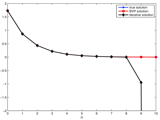
Figure 1: Solution of problem (1) computed by Miller’s algorithm.

Even using the term “stability” in the vague definition often used in Numerical Analysis, it is evident that the BVP solution is much more stable than the IVP solution. To be more precise, the characteristic polynomial of (1) has one root inside the unit circle and one outside. It cannot be considered stable according to the definition reported in Footnote 2. But why does it turn out to be stable for the BVP? The answer is simple: the definition of stability only concerns IVPs. For BVPs one must use the more general concept of conditioning. We do not report here the details (see, e.g. [38]). Once this new and more precise concept is used, then all the above questions become clear. Coming back to the above example, it turns out that a difference equation with one root inside and the other outside the unit circle is well conditioned if the two conditions that guarantee the uniqueness of its solution are placed one at the initial point and the other at the final point. This is enough not only to explain the result of the example, but also to explain, for example, the poor performances of the celebrated shooting method for solving continuous BVPs (see [38]).

Miller’s algorithm was deeply studied later on (see, e.g. [26, 16, 50, 51, 46, 47]) and eventually applied to design methods for ODEs, according to Dahlquist’s suggestion. For details, see [14] and references therein.

2.2 Abundance of $A$-stable methods

Once the vague concept of stability in Dahlquist’s proposal became more precise with the introduction of the conditioning notion, the definition of a great variety of $A$-stable LMMs followed. Of course, the definition of absolute stability, which requires that the asymptotic behaviour of the numerical solution be the same as that of the theoretical one, in relation to the test equation $y^{\prime}=\lambda y$, $\Re(\lambda)<0$, needed to be generalized accordingly.

Definition 1

A $k$-step LMM coupled with $k_{1}$ initial conditions and $k_{2}$ final conditions ($k=k_{1}+k_{2}$), is absolutely stable at $q=h\lambda$, if the characteristic polynomial has $k_{1}$ roots inside the unit circle and $k_{2}$ roots outside.

In other words, the requirement that all the roots of the characteristic polynomial of the difference equation defining the methods must be inside the unit circle was too much restrictive. The freedom to have some of them outside the unit circle opens wide possibilities. The only cost to pay is to shift some additional conditions to the end of the interval. Such methods have been called Boundary Value Methods (BVMs) (see, e.g. [14]). We are now plenty of $A$-stable linear multistep methods: even the methods with the highest possible order with respect to the given number of steps (Top Order Methods) are $A$-stable.

The above result has made it possible to write efficient codes for stiff (multiscale) problems based on LMMs (the codes GAM, GAMD, GAMP [36, 37] BIM, BIMD [4, 5], and TOM. See also the Test Set for IVP Solvers [48] for benchmarks of the most popular codes for ODEs).

3 Stiffness

Stiffness is a mathematical term to denote multiscale problems. At least, this was the first meaning of the term, although during the years the terms has been used in a great variety of meanings (for a historical account see [11]). A common way this term is perceived currently, is the following: a stiff problem is a problem for which explicit methods do not work. It is glaringly evident the inadequacy of such definition both for the mathematical needs and for logical reasons.

Despite the mentioned variety of definitions, the design of powerful codes needs a very precise definition of stiff problems, in order to be able to automatically recognize them and choose the appropriate strategies (appropriate methods, mesh selections, etc.). The situation assumes a paradoxical aspect: from the one hand some experts claim the impossibility of giving the needed precise definition of stiffness, and from the other, such definition does exist and is also published in a book [14, pp. 237 ff.]. The reason of such reluctance in accepting the mentioned precise definition stays, in our optimistic opinion, in the fact that the definition is based on a very simple idea, as we shall see soon. Fortunately, things are changing in recent years since the new definition has been used to improve the performance of some celebrated codes [15, 17, 18, 19].

3.1 The simple new idea

The two plots in Figure 2 report two functions: one constant and the other rapidly variable. How is it possible to distinguish their behaviors without looking at them? Simply, just compute the areas under their graphs and compare the results. Let $T$ be the interval, for technical reasons we normalize the two areas by dividing them by $T$. We get, respectively,

$$\kappa_{c}=\frac{T|y_{0}|}{T}=|y_{0}|;\quad\gamma_{c}=\frac{1}{T}\int_{0}^{T}|y(t)|dt.$$ (2)

  

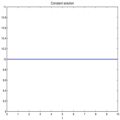
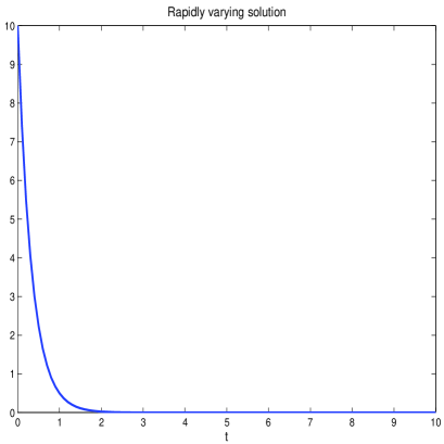
Figure 2: Functions with different behaviors: constant (left plot) and rapidly varying (right plot).

Suppose that $y(t)=e^{\lambda t}y_{0}$ with $\lambda$ negative. We get:

$$\gamma_{c}=\frac{1-e^{\lambda T}}{T|\lambda|}|y_{0}|<\frac{1}{T|\lambda|}|y_{0}|.$$

The ratio

$$\sigma_{c}=\frac{\kappa_{c}}{\gamma_{c}}\simeq\frac{T}{\frac{1}{|\lambda|}}$$

is the ratio of two times: the integration interval ($T$) and the decaying time ($\frac{1}{|\lambda|}$). Of course, the important case is the one in which the two types of solutions occur in the same problem. The quantity $\sigma_{c}$ measures the stiffness (or the multiscalarity) of the problem. The simple definition given above has been generalized to more general differential problems, autonomous and non autonomous dissipative problems, conservative problems, etc. (see [11, 12, 13, 14, 38]). Of course the extension of the definition to more general problems needs the introduction of more involved technicalities, but the leading idea remains unchanged: the definition of stiffness needs two measures, such as the infinity norm ($\kappa_{c}$) and the $L_{1}$ norm ($\gamma_{c}$), and the ratio between the two.

The above definition of stiffness deals with the continuous case. Of course, a very similar definition can be introduced for discrete problems, thus leading to the corresponding parameters $\kappa_{d}$, $\gamma_{d}$, $\sigma_{d}$. The two set of parameters (called conditioning parameters), turn out to be useful also to tell if the discrete problem is appropriate for approximating the corresponding continuous one. In fact one has:

Definition 2

A continuous problem is well represented by a discrete one if $\kappa_{c}\simeq\kappa_{d}$ and $\gamma_{c}\simeq\gamma_{d}$.

The use of the above precise definition, based on computable conditioning parameters, has allowed:

• to automatically recognize stiff problems;

• to define efficient variable mesh selection strategies.

As was pointed out above, some existing codes and new ones take advantage from the use of these conditioning parameters [13, 15, 17, 18, 19, 20, 43, 44, 45].

4 Hamiltonian Problems

Hamiltonian problems form a subclass of conservative problems. They assume the form

$$\frac{dy}{dt}=J\nabla H(y),\quad J=\left(\begin{array}[]{cc}0&I_{m}\\ -I_{m}&0\end{array}\right),\quad y(t_{0})=y_{0},$$ (3)

where $y=(q^{T},p^{T})^{T}$, $q,p\in{\mathbb{R}}^{m}$, and $H$ is a sufficiently smooth scalar function.

As was observed in the introduction, the main difficulty in dealing with them numerically stems from the fact that the meaningful isolated critical points of such systems are only marginally stable: neighboring solution curves do not eventually approach the equilibrium point either in future or in past times.

This implies that the geometry around them critically depends on perturbations of the linear part. Consequently, the use of a linear test equation, which essentially captures the geometry of the linear part, whose utility has been enormous in settling the dissipative case, cannot be of any utility in the present case.

It is then natural to look for other properties of Hamiltonian systems that can be imposed on the discrete methods in order to make them efficient. The first property which comes to mind is the symplecticity of the flow $\varphi_{t}:=y_{0}\mapsto y(t)$ associated with (3). This property can be described either in geometric form (invariance of areas, volumes, etc.) or in analytical form:

$$\left(\frac{\partial\varphi_{t}}{\partial y_{0}}\right)^{T}J\left(\frac{\partial\varphi_{t}}{\partial y_{0}}\right)=J.$$

In one way or the other, it essentially consists in moving infinitesimally on the trajectories representing the solutions. Infinitesimally means retaining only the linear part of the infinitesimal time displacement $\delta t$. It can be shown that this produces new values of the variables $q+\delta q,$ $p+\delta p$ which leave unchanged the value of the Hamiltonian $H(q+\delta q,p+\delta p)=H(q,p)$ (Infinitesimal Contact Transformation (ICT, see [28, p. 386])).

Consequently, since the composition of two or more such infinitesimal transformations maintain the invariance, so does an infinite number of them. The beauty of such result in the continuous case has perhaps created the expectation that similar beautiful achievements could be obtained in the discrete case. It is not surprising that the first attempts, to numerically approach the problem, aimed at devising symplectic integrators ([55, Ruth (1983)] , [25, Feng Kang (1985)]; see also the monographs [56, 42, 33] for more details on the subject).

Although in particular circumstances, for example in the case of quadratic Hamiltonians or, more in general, in the case of Hamiltonian systems admitting quadratic first integrals, this approach has provided very good results, it cannot be considered conclusive in treating general Hamiltonian problems.

A backward error analysis has shown that symplecticity somehow improves the long-time behavior properties of the numerical solutions. For a symplectic method of order $p$, implemented with constant stepsize $h$, the following estimation reveals how the numerical solution $y_{n}$ may depart from the manifold $H(y)=H(y_{0})$ of the phase space:

$$H(y_{n})-H(y_{0})=O(nh\,e^{-\frac{h_{0}}{2h}}h^{p}),$$ (4)

where $h_{0}>0$ is sufficiently small and $h\leq h_{0}$. Relation (4) implies that a linear drift of the energy with respect to time $t=nh$ may arise. However, due to the presence of the exponential, such a drift will not appear as far as $nh\leq e^{\frac{h_{0}}{2h}}$: this circumstance is often referred to by stating that symplectic methods conserve the energy function on exponentially long time intervals (see, for example, [33, Theorem 8.1]). This is clearly a surrogate of the definition of stability in that the “good behaviour” of the numerical solution is not extended on infinite time intervals. Even more alarming is the fact that if one wants to compute the numerical solution over very long times (as is done, for example, in the study of the stability of the Solar System), on the basis of (4), he may be obliged to reduce the stepsize below a safety threshold, which is in contrast with the spirit of the long time simulation of dynamical systems where the use of very large stepsizes is one of the primary prerogatives.

Where is the weakness of the approach? It is just in the above outlined words infinitesimal and infinite, which should be prohibited in Numerical Analysis. This discipline, in fact, has to deal with nonzero (greater than machine precision) and finite (bounded either by the patience of the operator or by the cost of energy) quantities. In other words, following this approach, the situation of the pre-Dahlquist era for dissipative problems has been recreated for conservative problems, in the sense that before Dahlquist there already existed methods, even with high order of convergence, that for $h$ small enough would do the job (for example, the midpoint and Simpson’s methods).

Coming back to linear problems, not all symplectic methods provide a conservation of the Hamiltonian function even in this simpler case: the following example has been taken from [14, Example 8.2.1 on p. 189]. Consider the harmonic oscillator problem in Hamiltonian form

$$\frac{d}{dt}\left(\begin{array}[]{c}q\\ p\end{array}\right)=J\left(\begin{array}[]{c}q\\ p\end{array}\right).$$ (5)

Let $h$ be the integration step and consider the numerical method defined by

$$\left(\begin{array}[]{c}q_{n+1}\\ p_{n+1}\end{array}\right)=M_{h}\left(\begin{array}[]{c}q_{n}\\ p_{n}\end{array}\right)\quad M_{h}=I+hJ-h^{2}\left(\begin{array}[]{cc}1&0\\ 0&0\end{array}\right).$$ (6)

Since the continuous solution in $h$ is $e^{hJ}y_{0},$ it is not difficult to deduce that the method is first order: $e^{Jh}-M_{h}=O(h^{2})$. The method is symplectic, since $M_{h}^{T}JM_{h}=J$, but fails to be conservative since, considering that $H(q,p)=(q,p)(q,p)^{T}/2$, we have

$$(q_{n+1},p_{n+1})\left(\begin{array}[]{c}q_{n+1}\\ p_{n+1}\end{array}\right)=(q_{n},p_{n})M_{h}^{T}M_{h}\left(\begin{array}[]{c}q_{n}\\ p_{n}\end{array}\right)\neq(q_{n},p_{n})\left(\begin{array}[]{c}q_{n}\\ p_{n}\end{array}\right).$$

The matrix $M_{h}$ is orthogonal only if the term $h^{2}$ is not present, according to the ICT hypothesis. But, unfortunately, this cannot be accepted since we want to use the method with finite values of $h$.

The literature about symplectic integrators is quite wide since Numerical Analysts, Physicists and Engineers have been working on them since more than 25 years. Consequently, this testifies their importance in the applications. However, other approaches have been attempted, among which:

• projection methods [3, 31] and numerical integrators on manifolds (see, e.g., [33, Sect. IV.5.3]);

• definitions of discrete counterparts of operators describing conservative vector fields, such as discrete gradients [29, 49], discrete divergence [39], averaged vector fields [54, 32], discrete line integrals [6] (see the next section for an introduction to the latter methods).

• generalizing the definition of symplecticity so as to include some nonlinearity in it (state dependent symplecticity [40]).

Remark 1

It is worth mentioning that a Hamiltonian system may have other constants of motion, consequently the following question arises: suppose that we are able to devise methods conserving the energy, are the methods also able to preserve, for example, quadratic invariants? Few results have been presented so far regarding essentially methods in the Runge-Kutta class, most of them rather pessimistic. The paper [10] gives a first positive answer to this issue.

From the above discussion it turns out that the problem considered is a very difficult one, although very important in the applications. The only solid result obtained in all these years seems to be the one establishing that, in order that a method can preserve the Hamiltonian functions, it must be symmetric (see, e.g., [14]), although, of course, this condition in not sufficient.

4.1 The simple new idea

The novel approach (see, for example [6] and references therein) starts from a trivial observation. Let $\omega(t)$ be any smooth curve $[t_{0},t_{1}]\rightarrow{\mathbb{R}}^{2m}$ passing through $y_{0}$ at time $t_{0}$. Then, we have:

$$H(\omega(t_{1}))-H(y_{0})=\int_{t_{0}}^{t_{1}}\frac{d}{dt}H(\omega(t))dt.$$ (7)

Of course, choosing $\omega(t)$ as the solution $y(t)$ to (3) yields

$$H(y(t_{1}))-H(y_{0})=\int_{t_{0}}^{t_{1}}\nabla^{T}H(y(t))\frac{dy(t)}{dt}\mathrm{d}t=\int_{t_{0}}^{t_{1}}\nabla^{T}H(y(t))J\nabla H(y(t))\mathrm{d}t=0.$$

The above result, which implies the conservation of the Hamiltonian function along the trajectory $y(t)$ at times $t_{0}$ and $t_{1}$, has been obtained by exploiting (3) and the skew-symmetry of the matrix $J$.

Is it possible to obtain a similar result for a curve $\omega(t)$ not coincident with the unknown solution $y(t)$ but nonetheless approximating it to a given order?

Surprisingly enough, the answer is positive. Let $\{\omega_{j}(t)\}_{j=0}^{\infty}$ be a set of linearly independent scalar functions defined on $[t_{0},t_{1}]$ and $\{\gamma_{j}\}_{j=0}^{r-1}$ a set of unknown vectors. For simplicity, we assume that

• the interval $[t_{0},t_{1}]$ coincides with $[0,1]$;

• the functions $\{\omega_{j}(t)\}_{j=0}^{\infty}$ are orthogonal;

• the integrals of such functions are easily expressible as linear combination of themselves.

By setting $\omega^{\prime}(t)=\sum_{i=0}^{r-1}\gamma_{i}\omega_{i}(t)$, we obtain

$$\omega(t)=y_{0}+\sum_{i=0}^{r-1}\gamma_{i}\int_{0}^{t}\omega_{i}(\tau)\mathrm{d}\tau\equiv y_{0}+\sum_{i=0}^{r^{\prime}}\tilde{\gamma_{i}}\omega_{i}(t).$$ (8)

The vectors $\tilde{\gamma_{j}}$, $j=0,\dots,r^{\prime}$ are uniquely determined in terms of linear combinations of the $\gamma_{i}$, $i=0,\dots,r-1$, according to the specific relations mentioned in item (3) above. Setting $y_{1}=\omega(1)$ yields

$$H(y_{1})-H(y_{0})=\sum_{i=0}^{r-1}\gamma_{i}^{T}\int_{0}^{1}\omega_{i}(t)\nabla H(\omega(t))\mathrm{d}t.$$

We now choose the $\{\gamma_{i}\}$ as the Fourier coefficients of the function $J\nabla H(\omega(t))$, i.e., we pose

$$\gamma_{i}=\eta_{i}\int_{0}^{1}\omega_{i}(t)J\nabla H(\omega(t))dt,\qquad i=0,\dots,r-1,$$ (9)

where $\{\eta_{i}\}$ are scalars that normalize the orthogonal functions $\{\omega_{i}(t)\}$ in order to make them an orthonormal basis for the space $L_{2}([0,1])$ of square-integrable functions. Considering the way the vectors $\{\gamma_{i}\}$ are involved in the definition of $\omega^{\prime}(t)$, we see that

$$\eta_{i}=\left(\int_{0}^{1}\omega_{i}^{2}(t)\mathrm{d}t\right)^{-1},\qquad i\geq 0.$$ (10)

Theorem 1

With the choice (9), the Hamiltonian assumes the same values at $y_{0}$ and at $y_{1}$.

Proof.  We have

$$H(y_{1})-H(y_{0})=\sum_{i=0}^{r-1}\eta_{i}\left[\int_{0}^{1}\omega_{i}(t)(\nabla H(\omega(t)))^{T}dt\right]J^{T}\left[\int_{0}^{1}\omega_{i}(t)\nabla H(\omega(t))dt\right]=0,$$

due to the fact that $J$ is skew-symmetric.  $\Box$

We have then proved that the Hamiltonian can be preserved on curves different from the solution. A rescaling of the form $[0,1]\rightarrow[t_{0},t_{0}+h]$ will introduce the stepsize $h$ and the iteration of the procedure will cover all the integration interval of interest with the result that on each interval of length $h$ there are at least two points (the end points) where the Hamiltonian assumes the same value.

The $r$ relations (9) define the unknown vectors $\{\gamma_{i}\}$ implicitly, since they appear as part of the integrands via the curve $\omega(t)$ in (8). Thus, in the general case, (9) have to be regarded as nonlinear integral equations. Therefore, in order to obtain a concrete numerical method we need:

• to substitute the integrals with discrete sums without introducing errors in the quadrature step;

• to design an algorithm to solve the resulting, usually nonlinear, system providing the $\{\gamma_{i}\}$;

• to check that the vector $y_{1}=\omega(t_{1})$, which will be assumed as an approximation, at time $t_{1}$, of the true solution $y(t_{1})$, has indeed the desired order of accuracy, say $p$: $||y(t_{1})-y_{1}||=O(h^{p+1})$, for a given integer $p\geq 1$.

More in general, step (a) could be replaced by the assumption that primitive functions for the integrands are available in closed form, no matter whether they can be expressed via standard quadrature formulae (see the examples in [8, Section 4]). In any event, the requirement (a) can be completely fulfilled if the functions $\{\omega_{i}(t)\}$ and $H$ are polynomials.

Let $\nu$ be the degree of $H(y)$, and $r-1$ be the degree of $\omega^{\prime}(t)$. Then the integrands in (9) are polynomials as well, of degree at most $\mu=r(\nu-1)+r-1=\nu r-1$. We need then quadrature formulae having degree of precision greater than or equal to $\mu$. Of course, it will be advantageous to chose them of Gaussian type.

As we will see in Subsection 4.3, the resulting methods fall in the class of block-BVMs and have been called Hamiltonian Boundary Value Methods (HBVMs).

To describe how the above three tasks can be accomplished, we start with the simpler case where $H(y)$ is a quadratic function and therefore problem (3) is linear. In particular, we will consider hereafter the harmonic oscillator problem realizing that the obtained method is in fact the Gauss-Legendre method. The approach will be then generalized to nonlinear Hamiltonians thus leading to the new formulae.

4.2 Application to the Harmonic Oscillator Problem

The harmonic oscillator problem is described in Eq. (5); note that $\nabla H(y)=(q,p)^{T}$. Of course, we are tempted to take as set $\{\omega_{i}(t)\}_{i=0}^{\infty}$ the trigonometric orthogonal systems, since this would provide the exact solution, even for small values of $r$.

Let us instead take for $\{\omega_{i}\}$ the set of shifted Legendre polynomials $\{P_{i}(t)\}$, which is orthogonal in $[0,1]$. They may be defined by the Rodrigues formula

$$P_{i}(t)=\frac{1}{i!}\frac{\mathrm{d}^{i}}{\mathrm{d}t^{i}}\left[(t^{2}-t)^{i})\right],\qquad i\geq 0$$

(we also set $P_{-1}(t)\equiv 0$). The first few are:

$$P_{0}(t)=1,\quad P_{1}(t)=2t-1,\quad P_{2}(t)=6t^{2}-6t+1,\quad P_{3}(t)=20t^{3}-30t^{2}+12t-1.$$

What we here need about such polynomials are the following two properties ($\delta_{ij}$ denotes the Kronecker symbol):

• $\int_{0}^{1}P_{i}(t)P_{j}(t)dt=\frac{1}{2i+1}\delta_{ij},\qquad i,j\geq 0$;

• $\int_{0}^{t}P_{j}(x)\mathrm{d}x=\frac{1}{2(2j+1)}(P_{j+1}(t)-P_{j-1}(t)+\delta_{j0}P_{0}(t)),\qquad j\geq 0$.

Comparing Property $(L_{1})$ with the normalization condition (10) yields $\eta_{i}=2i+1$. In this example we set $r=3$ and, hence,

$$\begin{array}[]{rcl}\omega^{\prime}(t)&=&P_{0}(t)\gamma_{0}+P_{1}(t)\gamma_{1}+P_{2}(t)\gamma_{2},\\[8.5359pt] \omega(t)&=&y_{0}+\frac{1}{2}(P_{1}(t)+P_{0}(t))\gamma_{0}+\frac{1}{6}(P_{2}(t)-P_{0}(t))\gamma_{1}+\frac{1}{10}(P_{3}(t)-P_{1}(t))\gamma_{2}.\end{array}$$

Relations (9) become

$$\begin{array}[]{rcl}\gamma_{1}&=&\frac{30}{59}J\gamma_{0},\\[8.5359pt] \gamma_{2}&=&\frac{1}{6}J\gamma_{1}~{}=~{}-\frac{5}{59}\gamma_{0},\\[8.5359pt] \gamma_{0}&=&\frac{1}{6}J(3\gamma_{0}-\frac{30}{59}J\gamma_{0}+6y_{0})~{}=~{}\frac{2\cdot 59}{4\cdot 54^{2}+59^{2}}(-59I+2\cdot 54J)y_{0},\end{array}$$

from which, by setting $S=\frac{1}{4\cdot 54^{2}+59^{2}}(-59I+2\cdot 54J)$, we obtain

$$\begin{array}[]{rcl}\omega^{\prime}(t)&=&\left((2\cdot 59P_{0}(t)-10P_{2}(t))I+60P_{1}(t)J\right)Sy_{0},\\[8.5359pt] \omega(t)&=&y_{0}+\left[(60P_{1}(t)+59P_{0}(t)-P_{3}(t))I+10(P_{2}(t)-P_{0}(t))J\right]Sy_{0}.\end{array}$$

and therefore the residual,

$$R(t)=\omega^{\prime}(t)-J\omega(t)=P_{3}(t)JSy_{0},$$

is zero (collocation) when $t$ is a root of $P_{3}(t)$. Since the roots of $P_{3}(t)$ are the abscissae of the Gauss collocation method of order six, from the uniqueness of the collocation polynomial we conclude that our approach applied to linear problems leads to these formulae.

Interestingly, this approach leads to completely new formulae if applied to general nonlinear Hamiltonian problems.

4.3 Hamiltonian Boundary Value Methods (HBVMs)

Relations (9) have been retrieved by imposing the energy conservation property at the end points of the curve $\omega(t)$, $t\in[t_{0},t_{0}+h]$, and we are now assuming that $H(y)$ is a polynomial of degree $\nu$ so that the integrals may be exactly evaluated, for example, by means of a Gaussian quadrature formula of sufficiently high degree. As was pointed out in Subsection 4.1 they form a block nonlinear system of dimension $r$ which, once solved, will provide the expression of the curve $\omega(t)$ and, hence, of the numerical solution at time $t_{1}=t_{0}+h$, namely $y_{1}=\omega(t_{0}+h)$. The resulting methods have been called Hamiltonian Boundary Value Methods (HBVMs) because they are naturally and conveniently recast as block-BVMs (see [8, 7] for more details about their formulation and implementation).

What about their order of convergence? Let us consider again the shifted Legendre polynomials. Substituting (9) into (8), and setting $c=(t-t_{0})/h$, yields

$$\omega(t_{0}+ch)=y_{0}+h\sum_{j=0}^{r-1}(2j+1)\int_{0}^{c}P_{j}(x)\mathrm{d}x\,\int_{0}^{1}P_{j}(\tau)f(\omega(t_{0}+\tau h))\mathrm{d}\tau$$ (11)

and, on differentiating with respect to $c$,

$$\omega^{\prime}(t_{0}+ch)=\sum_{j=0}^{r-1}(2j+1)P_{j}(c)\,\int_{0}^{1}P_{j}(\tau)f(\omega(t_{0}+\tau h))\mathrm{d}\tau.$$ (12)

In the above relations, we have set $f(y)\equiv J\nabla H(y)$.

Both (11) and (12) have an interesting interpretation. Consider the unknown solution $y(t_{0}+ch)$ of

$$\left\{\begin{array}[]{l}y^{\prime}(t_{0}+ch)=f(y(t_{0}+ch)),\qquad c\in[0,1],\\ y(t_{0})=y_{0},\end{array}\right.$$ (13)

or, equivalently, of its integral formulation

$$y(t_{0}+ch)=y_{0}+h\int_{0}^{c}f(y(t_{0}+\tau h))\mathrm{d}\tau.$$ (14)

Let us consider the Fourier series of $f(y(t_{0}+\tau h))$ for $\tau\in[0,1]$:

$$f(y(t_{0}+ch))=\sum_{j=0}^{\infty}(2j+1)P_{j}(c)\int_{0}^{1}P_{j}(\tau)f(y(t_{0}+\tau h))\mathrm{d}\tau.$$ (15)

In terms of such expansion, (13) and (14) read

$$\left\{\begin{array}[]{l}y^{\prime}(t_{0}+ch)=\displaystyle\sum_{j=0}^{\infty}(2j+1)P_{j}(c)\int_{0}^{1}P_{j}(\tau)f(y(t_{0}+\tau h))\mathrm{d}\tau,\qquad c\in[0,1],\\ y(t_{0})=y_{0},\end{array}\right.$$ (16)

and

$$y(t_{0}+ch)=y_{0}+h\sum_{j=0}^{\infty}(2j+1)\int_{0}^{c}P_{j}(x)\mathrm{d}x\,\int_{0}^{1}P_{j}(\tau)f(y(t_{0}+\tau h))\mathrm{d}\tau,$$ (17)

respectively. Consequently (11) and (12) are defined by simply truncating the series on the right hand side of (16) and (17). Of course, in the event that series (15) actually contains a finite number of terms, there will be no difference between (16)-(17) and (13)-(14), provided $r$ is large enough.

How close are the two set of problems? The answer is obtained by means of the Alekseev formula [1], by using the following preliminary result.

Lemma 1

Let $g$ be a suitably regular function and $h>0$. Then

$$\int_{0}^{1}P_{j}(\tau)g(\tau h)\,\mathrm{d}\tau=O(h^{j}),\qquad j\geq 0.$$

Proof.  Assume, for sake of simplicity,

$$g(\tau h)=\sum_{n=0}^{\infty}\frac{g^{(n)}(0)}{n!}(\tau h)^{n}$$

to be the Taylor expansion of $g$. Then, for all $j\geq 0$,

$$\int_{0}^{1}P_{j}(\tau)g(\tau h)\,\mathrm{d}\tau=\sum_{n=0}^{\infty}\frac{g^{(n)}(0)}{n!}h^{n}\int_{0}^{1}P_{j}(\tau)\tau^{n}\,\mathrm{d}\tau=O(h^{j}),$$

since $P_{j}$ is orthogonal to polynomials of degree $n<j$. $\Box$

Let us now define the functions

$$F_{h}(c,y)=\sum_{j=0}^{r-1}(2j+1)P_{j}(c)\int_{0}^{1}P_{j}(\tau)f(y(t_{0}+\tau h))\mathrm{d}\tau$$ (18)

and

$$R_{h}(c,y)=\sum_{j=r}^{\infty}(2j+1)P_{j}(c)\int_{0}^{1}P_{j}(\tau)f(y(t_{0}+\tau h))\mathrm{d}\tau.$$ (19)

From Lemma 1, after setting $g(\tau h)=f(y(t_{0}+\tau h))$, we deduce that

$$R_{h}(c,y)=\sum_{j=r}^{\infty}a_{j}(h)P_{j}(c),$$ (20)

with $a_{j}(h)=O(h^{j})$, $j=r,r+1,\dots$ and, therefore, $R_{h}(c,y)=O(h^{r}).$

Moreover, for any given $\tilde{t}\in[t_{0},t_{0}+h]$, we denote by $\omega(s,\tilde{t},\tilde{y})$ the solution of (12) at time $s$ and with initial condition $\omega(\tilde{t})=\tilde{y}$.

Lemma 2 (Alekseev (1961))

Consider the two initial value problems with the same initial condition

$$\begin{array}[]{ll}z^{\prime}=\varphi(t,z),&z(t_{0})=y_{0},\\ y^{\prime}=\varphi(t,y)+\psi(t,y),&y(t_{0})=y_{0},\\ \end{array}$$

and suppose that $\varphi$ is continuously differentiable with respect to the second argument. Then the two solutions $z(t)$ and $y(t)$ satisfy the following relation:

$$y(t)-z(t)=\int_{t_{0}}^{t}\frac{\partial z}{\partial y_{0}}(t,c,y(c))\,\psi(c,y(c))\,\mathrm{d}c.$$ (21)

Proof.  See, for example, [33, Theorem 14.5, p. 96] or [41, Theorem 7.5.1, p. 205]. $\Box$

We can now state the following result.

Theorem 2

Let $\omega(t_{0}+ch)$ and $y(t_{0}+ch)$, $c\in[0,1]$, be the solutions of (12) and (16), respectively. Then,

$$y(t_{0}+h)-\omega(t_{0}+h)=O(h^{2r+1}).$$

Proof.  In terms of the functions $F_{h}$ and $R_{h}$, problems (12) and (16) read

$$\omega^{\prime}(t_{0}+ch)=F_{h}(c,\omega),\qquad y^{\prime}(t_{0}+ch)=F_{h}(c,y)+R_{h}(c,y),$$

respectively. From the Alekseev formula (21) one then obtains, by virtue of Lemma 1 and (20), that

$$y(t_{0}+h)-\omega(t_{0}+h)=$$

$$= h\int_{0}^{1}\frac{\partial\omega}{\partial y_{0}}(t_{0}+h,t_{0}+\tau h,y(t_{0}+\tau h))\,R_{h}(\tau,y)\,\mathrm{d}\tau$$

$$= h\sum_{j=r}^{\infty}\left(\int_{0}^{1}P_{j}(\tau)\frac{\partial\omega}{\partial y_{0}}(t_{0}+h,t_{0}+\tau h,y(t_{0}+\tau h))\,\mathrm{d}\tau\right)a_{j}(h)$$

$$= h\,O(h^{r})\,O(h^{r})=O(h^{2r+1}).~{}\mbox{$\Box$}$$

As a direct consequence, we obtain the following result.

Corollary 1

Let $T=Nh$ be a fixed positive real number, $N$ being an integer. Then, the approximation to the solution of problem

$$y^{\prime}(t)=f(y(t)),\qquad t\in[t_{0},t_{0}+T],\qquad y(t_{0})=y_{0},$$

by means of

$$\omega^{\prime}(t_{i-1}+ch)=\sum_{j=0}^{r-1}(2j+1)P_{j}(c)\int_{0}^{1}P_{j}(\tau)f(\omega(t_{i-1}+ch))\,\mathrm{d}\tau,\quad c\in[0,1],\quad i=1,\dots,N,$$

where  $t_{i}=t_{i-1}+h$,  $i=1,\dots,N$,  and  $\omega(t_{0})=y_{0}$,  is  $O(h^{2r})$  accurate.

4.4 A numerical example

In order to make clear the advantage of using the energy-preserving HBVMs (12) over standard symplectic methods, we just mention that standard mesh selection strategies are not advisable for symplectic methods (see, e.g., [56, p. 127], [42, p. 235], [33, p. 303]), since a drift in the Hamiltonian and a quadratic error growth is experienced in such a case. The example that we consider below gives a hint that this is not the case for HBVMs, provided that the integral in (12) is exactly computed (at least, numerically which, as observed before, can be always achieved, for all suitably regular Hamiltonian functions).

Remark 2

As also observed in Section 4.2, we mention that when the integrals in (12) are approximated by means of the Gauss-Legendre formula with $r$ points, then the Gauss-Legendre method of order $2r$ is obtained [8].

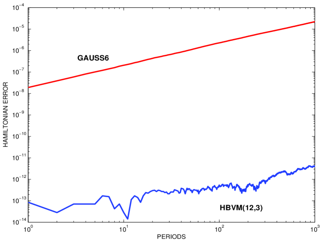
Figure 3: Hamiltonian error growth over 1000 periods with a variable-step solution of problem (22)–(23), $e=0.99$, with tolerance $tol=10^{-10}$.

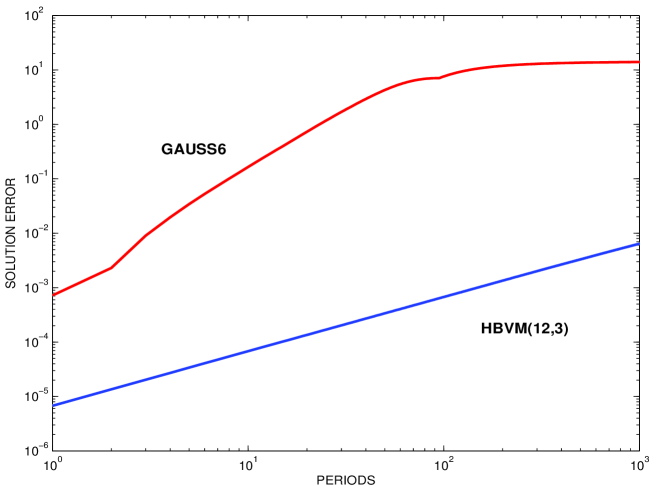
Figure 4: Error growth over 1000 periods with a variable-step solution of problem (22)–(23), $e=0.99$, with tolerance $tol=10^{-10}$.

We now consider the Kepler problem (see, e.g., [33, p. 9]), with Hamiltonian

$$H([q_{1},\,q_{2},\,p_{1},\,p_{2}]^{T})=\frac{1}{2}(p_{1}^{2}+p_{2}^{2})-\frac{1}{\sqrt{q_{1}^{2}+q_{2}^{2}}},$$ (22)

that, when started at

$$\left(\begin{array}[]{cccc}1-e,&0,&0,&\sqrt{\frac{1+e}{1-e}}\end{array}\right)^{T},$$ (23)

has an elliptic periodic orbit of period $2\pi$ and eccentricity $e\in[0,1)$. Moreover, in such a case, the (constant) value of the Hamiltonian is $H_{0}=-\frac{1}{2}$. When $e$ is close to 0, the problem is efficiently solved by using a constant stepsize. However, it becomes more and more difficult as $e\rightarrow 1$, so that a variable-step integration would be more appropriate in this case. In Figures 3 and 4 we plot the error growth in the Hamiltonian and in the solution, respectively, over 1000 periods, in the case $e=0.99$, when using a standard mesh selection strategy (e.g., like (1.1) in [33, p. 303]) with the (symplectic) Gauss-Legendre method of order 6 and the HBVM (12) with $r=3$ (then, again of order 6), where the integral is approximated by means of a Gauss formula with $k=12$ points, then having order 24, which is sufficient to obtain, in this case, a practical energy conservation (see [6], and references therein, for full details). The latter method is in general denoted by HBVM$(k,r)$ [6], so that in the present case we consider the HBVM(12,3) method. The tolerance used is $tol=10^{-10}$. As one can see, the Gauss-Legendre formula produces a drift in the Hamiltonian and a quadratic error growth, whereas the HBVM(12,3) exhibits a negligible error in the Hamiltonian and a linear error growth. This confirms that the symplectic Gauss-Legendre method is more conveniently used with a constant stepsize, whereas the energy preserving HBVM can be profitably used with a standard mesh selection strategy.

Table 1: Statistics for the variable step implementation of HBVM(12,3) on the Kepler problem (22)–(23), $e=0.99$, with tolerance $tol=10^{-10}$.

periods error points 100 6.75e-04 15300 200 1.36e-03 30600 300 2.04e-03 45900 400 2.72e-03 61200 500 3.41e-03 76500 600 4.10e-03 91800 700 4.79e-03 107100 800 5.48e-03 122400 900 6.17e-03 137700 1000 6.85e-03 153000

In Table 1 we also list the number of points required by the HBVM(12,3) method, with variable stepsize, for covering an increasing number of periods: as one can easily deduce from the listed data, 153 steps are required to cover each period. In order to make clear the improvement over the symplectic sixth-order Gauss method, it is enough to observe that, in order to obtain a comparable accuracy, this method would require approximately $2\cdot 10^{5}$ (constant) steps for each period!

5 Conclusions

We have reported three problems in Numerical Analysis considered difficult for as long as half a century and which, in our opinion, have been eventually resolved by dramatically changing the traditional approach suggested by experience. We reiterate that this is certainly due to the fact that past studies were heavily biased by the concept of continuity, whose peculiarities the researchers have tried to import in the new context of Numerical Analysis, where such problems are, instead, of discrete nature: the two areas, i.e., the continuous one and the discrete one, are often not overlapping.

Within this scenario, although it’s certainly easier to follow the tracks already drawn and consolidated in the literature, exploring new routes sometimes allows to reach the goal more quickly and innovatively, as picturesquely described in the tale of the egg of Columbus.

References

- [1] V.M. Alekseev, An estimate for the perturbations of the solution of ordinary differential equations (Russian), Vestn. Mosk. Univ., Ser.I, Math. Meh, 2 (1961) 28–36.
- [2] D.S. Alexander, F. Iavernaro and A. Rosa, “Early Days in Complex Dynamics,” AMS-LMS History of Mathematics, (to appear).
- [3] U. Ascher and S. Reich, On some difficulties in integrating highly oscillatory Hamiltonian systems, in “Computational Molecular Dynamics”, Lect. Notes Comput. Sci. Eng. 4, Springer, Berlin, (1999), 281–296.
- [4] L. Brugnano and C. Magherini, The BiM code for the numerical solution of ODEs, J. Comput. Appl. Math. 164–165 (2004) 145–158.
- [5] L. Brugnano and C. Magherini, Blended implicit methods for solving ODE and DAE problems, and their extension for second order problems, J. Comput. Appl. Math. 205 (2007) 777–790.
- [6] L. Brugnano, F. Iavernaro and D. Trigiante, The Hamiltonian BVMs (HBVMs) Homepage, arXiv:1002.2757.
- [7] L. Brugnano, F. Iavernaro and D. Trigiante, Analisys of Hamiltonian Boundary Value Methods (HBVMs): a class of energy-preserving Runge-Kutta methods for the numerical solution of polynomial Hamiltonian dynamical systems, BIT (2009) submitted (arXiv:0909.5659).
- [8] L. Brugnano, F. Iavernaro and D. Trigiante, Hamiltonian Boundary Value Methods (Energy Preserving Discrete Line Integral Methods), Jour. of Numer. Anal. Industr. and Appl. Math. (2010) to appear (arXiv:0910.3621).
- [9] L. Brugnano, F. Iavernaro and D. Trigiante, Isospectral Property of HBVMs and their connections with Runge-Kutta collocation methods, Preprint (2010) (arXiv:1002.4394).
- [10] L. Brugnano, F. Iavernaro and D. Trigiante, On the existence of energy-preserving symplectic integrators based upon Gauss collocation formulae, submitted (2010) (arXiv:1005.1930).
- [11] L. Brugnano, F. Mazzia and D. Trigiante, Fifty Years of Stiffness. Chapter 1 in Recent Advances in Computational and Applied Mathematics, T.E. Simos Ed., Springer, 2011.
- [12] L. Brugnano and D. Trigiante, On the characterization of Stiffness, Dynamics of Cont., Discr. Impuls. Systems 2 (1996) 317–335.
- [13] L. Brugnano and D. Trigiante, A new mesh selection strategy for ODEs, Appl. Numer. Math. 24 (1997) 1–21.
- [14] L. Brugnano and D. Trigiante, “Solving ODEs by Linear Multistep Initial and Boundary Value Methods,” Gordon and Breach, Amsterdam, 1998.
- [15] S.Capper, J.R. Cash and F. Mazzia, On the development of effective algorithms for the numerical solution of singularly perturbed two-point boundary value problems, Int. Journ. of Comput. Science and Math. 1 (2007) 42–57.
- [16] J. Cash, “Stable recursions. With applications to numerical solution of stiff systems,” Academic Press., London (1979).
- [17] J.R. Cash and F. Mazzia, A new mesh selection algorithm, based on conditioning, for two-point Boundary Value Codes, Jour. Comput. Appl. Math., 184 (2005) 362–381.
- [18] J.R. Cash and F. Mazzia, Hybrid mesh selection algorithms based on conditioning for two-point boundary value problems, J. Numer. Anal. Ind. Appl. Math., 1 (2006) 81–90.
- [19] J.R. Cash and F. Mazzia, Conditioning and Hybrid Mesh Selection Algorithms for Two-Point Boundary Value Problems, Scalable Computing: Practice and Experience, 10 (4) (2009) 347–361.
- [20] J.R. Cash and F. Mazzia, Algorithms for the solution of two-point boundary value problems, http://www.ma.ic.ac.uk/~jcash/BVP˙software/twpbvp.php
- [21] G.F. Curtiss and J.O. Hirshfelder, Integration of stiff equations, Proc. Nat. Acad. Science U.S. 38 (1952), 235–243.
- [22] G. Dahlquist and Ä. Björck, “Numerical Methods”, Prentice Hall, Englewood Cliffs, N.J., 1974.
- [23] G. Dahlquist, A special stability problem for linear multistep methods, BIT 3 (1964), 27–43.
- [24] G. Dahlquist, 33 years of instability, Part I, BIT 25 (1985), 188–204.
- [25] K. Feng, On difference schemes and symplectic geometry, in Proceedings of the 5-th Intern. Symposium on differential geometry & differential equations, August 1984, Beijing (1985), 42–58.
- [26] W. Gautschi, Computational aspects of three-term recurrence relations, SIAM Rev. 9 (1967), 24–82.
- [27] W. Gautschi, “Numerical Analysis, An introduction,” Birkhäuser Boston, Inc., Boston, MA, 1997.
- [28] H. Goldstein, C.P. Poole and J.L. Safko, “Classical Mechanics,” Addison Wesley, 2001.
- [29] O. Gonzalez, Time integration and discrete Hamiltonian systems, J. Nonlinear Sci. 6 (1996), 449–467.
-
[30]
N. Guglielmi and E. Hairer (2007), Scholarpedia 2(11):2850,
revision # 64754.
http://www.scholarpedia.org/article/Stiff˙delay˙equations - [31] E. Hairer, Symmetric projection methods for differential equations on manifolds, BIT 40 (2000), 726–734.
- [32] E. Hairer, Energy-preserving variant of collocation methods, J. Numer. Anal. Ind. Appl. Math., to appear.
- [33] E. Hairer, C. Lubich and G. Wanner, “Geometric Numerical Integration. Structure-Preserving Algorithms for Ordinary Differential Equations,” Second ed., Springer, Berlin, 2006.
- [34] A.C. Hindmarsh, “On Numerical Methods for Stiff Differential Equations–Getting the Power to the People,” Lawrence Livermore Laboratory, UCRL-83259, 1979.
- [35] W.H. Hundshorfer, The numerical solution of stiff initial value problems: an analysis of one step methods, CWI Tracts 12 Amsterdam (1980).
- [36] F. Iavernaro and F. Mazzia, Solving ordinary differential equations by generalized adams methods: properties and implementation techniques, Appl. Numer. Math. (2–4) 28 (1998), 107–126.
- [37] F. Iavernaro and F. Mazzia, On the extension of the code GAM for parallel computing, in EURO-PAR’99, Parallel Processing, Lecture Notes in Computer Science, 1685, Springer, Berlin (1999), 1136–1143.
- [38] F. Iavernaro, F. Mazzia and D. Trigiante, Stability and conditioning in Numerical Analysis, JNAIAM 1 (2006), 91–112.
- [39] F. Iavernaro and D. Trigiante, Discrete conservative vector fields induced by the trapezoidal method. J. Numer. Anal. Ind. Appl. Math. 1 (2006), 113–130.
- [40] F. Iavernaro and D. Trigiante, State-dependent symplecticity and area preserving numerical methods, J. Comput. Appl. Math. (2) 205 (2007), 814–825.
- [41] V. Lakshikantham and D. Trigiante, “Theory of Difference Equations. Numerical Methods and Applications,” Second Edition, Marcel Dekker, New York (2002).
- [42] B. Leimkuhler and S. Reich, “Simulating Hamiltonian Dynamics”, Cambridge University Press 2004.
-
[43]
F. Mazzia, Software for Boundary value Problems,
(2003),
http://www.dm.uniba.it/~mazzia/bvp/index.html - [44] F. Mazzia, A. Sestini and D. Trigiante., The continous extension of the -spline linear multistep metods for BVPs on non-uniform meshes, Appl. Numer. Math., 59(3–4) (2009) 723–738.
- [45] F. Mazzia and D. Trigiante, A Hybrid Mesh Selection Strategy Based on Conditioning for Boundary Value ODE Problems, Numerical Algorithms 36 (2004) 169–187.
- [46] R.M.M. Mattheij, Characterizations of dominant and dominated solutions of linear recursions, Numer. Math. 35 (1980), 421–442.
- [47] R.M.M. Mattheij, Stable computation of solutions of unstable linear initial value recursions, BIT 22 (1982), 79–93.
-
[48]
F. Mazzia and C. Magherini, Test Set for IVP Solvers, rel. 2.4, (2008),
http://dm.uniba.it/~testset/ - [49] R.I. McLachlan, G.R.W. Quispel and N. Robidoux, Geometric integration using discrete gradient, Phil. Trans. R. Soc. Lond. A 357 (1999), 1021–1045.
- [50] J. Oliver, The numerical solution of linear recurrence relations, Numer. Math. 11 (1968), 349–360.
- [51] F.W.J. Olver, Numerical solution of second-order linear difference equations, J. Res. Nat. Bur. Standards 71B (1967), 111-129.
-
[52]
L. Petzold et al., Report on the First Multiscale
mathematics Workshop: First Steps towards a Roadmap, 2004,
http://www.mcs.anl.gov/~gropp/bib/reports/Multiscale-sept04.pdf - [53] H. Poincaré, Sur les courbes définies par une équation différentielle, J. de Mathématiques pures et appliquées, quatrième partie (4) 2 (1886), 151–217.
- [54] G.R.W. Quispel and D.I. McLaren, A new class of energy-preserving numerical integration methods, J. Phys. A: Math. Theor. 41 (2008) 045206 (7pp).
- [55] R.D. Ruth, A canonical integration technique, IEEE Trans. Nuclear Science NS-30 (1983), 2669–2671.
- [56] J.M. Sanz-Serna and M.P. Calvo, “Numerical Hamiltonian Problems,” Chapman & Hall, London, 1994.