Abstract

Taking advantage of the electron Bernstein waves heating (EBWH) system of the TJ–II stellarator, an electron Bernstein emission (EBE) diagnostic was installed. Its purpose is to investigate the B–X–O radiation properties in the zone where optimum theoretical EBW coupling is predicted. An internal movable mirror shared by both systems allows to collect the EBE radiation along the same line of sight that is used for EBW heating. The theoretical EBE has been calculated for different orientations of the internal mirror using the TRUBA code as ray tracer. A comparison with experimental data obtained in NBI discharges is carried out. The results provide a valuable information regarding the experimental O–X mode conversion window expected in the EBW heating experiments. Furthermore, the characterization of the radiation polarization shows evidence of the underlying B–X–O conversion process.

1 Introduction

Plasma heating by Electron Bernstein waves [1] has been successfully demonstrated in several magnetic confinement devices [2, 3, 4, 5]. The main advantage of this technique is that it offers the possibility to heat plasmas above the density limits of the standard electromagnetic modes. For a complete review of the EBW topic see [6] and references therein. Moreover, the emitted Bernstein waves from the over-dense plasma core can be helpful for the plasma diagnosis in high density scenarios. See, for instance, ref. [7], where EBE is used as an electron temperature diagnostic and ref. [8] where it is employed to measure the magnetic field.

The TJ–II stellarator [9] is a medium size heliac with major radius $R_{0}=1.5$ m, minor radius $a\approx 0.2$ m and magnetic field strength on axis around $0.95$ T. In this device, the use of the available ECR heating sources –two gyrotrons delivering 300 kW power each and injecting X–mode polarized waves at second harmonic ($f=53.2$ GHz)– is limited by the cut-off density for that frequency and that mode, i.e. $n_{e}\approx 1.7\times 10^{19}$ m^-3. Two neutral beam injectors allow to heat the plasma above this limit and therefore, additional ECRH heating in NBI plasmas becomes possible only through electron Bernstein waves. The heating scheme using Bernstein waves for TJ-II is based on the O–X–B double mode conversion using low field side launching [10].

As it is well-known, the efficiency of the O–X mode conversion depends strongly on the launching direction and the polarization of the incident wave. Thus, in order to find an optimum experimental heating efficiency, a steerable mirror was installed inside the vacuum vessel, allowing a horizontal and vertical scan of the ECRH beam launching direction around the direction for which maximum O–X mode conversion efficiency is expected. Note that a perfect optimization procedure should also include the displacement of the mirror center, since for each penetration location of the plasma wave a different well defined injection direction is required. This is not possible with the existing design.

In the present setup, the mirror can also be positioned so that the plasma radiation coming along the EBWH launching direction is redirected towards a radiometer antenna that measures thermal emission at 28 GHz. With this setup, measuring and heating can not be performed at the same time. Since both the EBWH and the ECE/EBE systems share the same line of sight, the analysis of electron cyclotron radiation in plasmas above the O mode cut-off density for 28 GHz ($n_{e}\approx 1.0\times 10^{19}$ m⁻³) may provide a very valuable information to determine the optimum direction for O–X–B heating. As a matter of fact, because of the low cut-off densities of the 28 GHz electromagnetic modes, any radiation detected in plasmas above this density must come from an inverse B–X–O mode conversion unless the contribution of the peripheral underdense plasma to the emission is high enough to mask the B–X–O component. This point will be addressed in the discussion.

In this work, we present the theoretical characterization of the EBE resulting from B–X–O conversion, for different orientations of the launching mirror and different rotation angles of the radiometer, in the vicinity of the position that provides the maximum theoretical O–X conversion efficiency. The numerical results are obtained with the ray tracing code TRUBA and the well-known concepts in traditional ECE calculations, i.e. energy balance between emission and absorption as well as black body approximation. The theoretical results are compared with the experimental ones, obtained under ECRH + NBI discharges.

The article is outlined as follows: section 2 focuses on the description of the experimental setup; section 3 deals with the numerical EBE calculations; section 4 is devoted to the experimental results and their comparison with the predictions presented in section 3; and finally, section 5 summarizes and discusses the main results. The appendix describes the calculation of the expected power in the different polarizations measured by the radiometer when it is rotated around its symmetry axis.

2 EBWH launching system and EBE diagnostic

The EBWH launching system consists of a corrugated waveguide that transmits up to 300 kW of microwave power into the vacuum vessel, where a steerable ellipsoidal mirror ($170$ mm $\times 190$ mm) focuses the beam and defines the launching direction. Prior to coupling the radiation to the waveguide, two elliptical focusing mirrors and two $\lambda/4$ and $\lambda/8$ plane polarizers provide a Gaussian beam with the properly

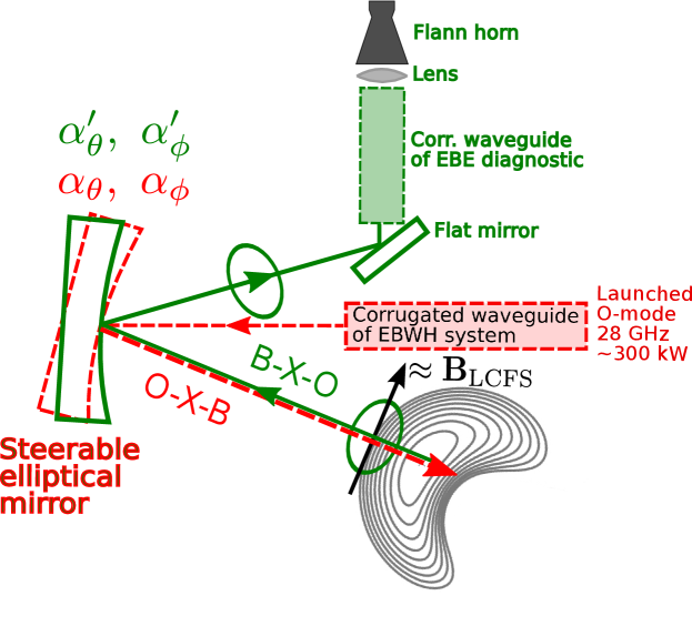
Figure 1: EBWH launching system and EBE diagnostic. Different mirror positioning angles are used for EBW heating ($\alpha_{\phi}$, $\alpha_{\theta}$) and for EBE detection ($\alpha_{\phi}^{\prime}$, $\alpha_{\theta}^{\prime}$). Radiated power suffers two consecutive reflections and is coupled to the detection waveguide.

polarized electromagnetic field. For the details of the EBW heating system see refs. [11, 12]. The position of the movable mirror is determined by two orientation angles along the horizontal (or toroidal) and vertical (or poloidal) directions, $\alpha_{\phi}$ and $\alpha_{\theta}$ respectively. If the launching direction is given by these angles, the radiation coming from this same direction can be redirected to the 28 GHz heterodyne radiometer using a different pair of angles $\alpha_{\phi}^{\prime}$ and $\alpha_{\theta}^{\prime}$ and a flat mirror attached to a corrugated waveguide, similar to the one used in the launching system (see figure 1). After its passing through a glass focusing lens located outside the vacuum chamber, the radiation is detected by a quad-ridged dual-polarized microwave horn. The lens modifies the beam pattern at the output of the waveguide in order to obtain an efficient coupling to the horn antenna. For further details of the EBE diagnostic see [13, 14].

Once the 28 GHz radiation reaches the horn, it is split into two separate components according to two orthogonal detection directions. Properly calibrated, the sum of both signals, $I_{\text{\tiny{EBE1}}}$ and $I_{\text{\tiny{EBE2}}}$, corresponds to the total radiative temperature $T_{\text{\tiny{rad}}}$. Accordingly to the properties of an obliquely propagating O mode, an elliptical polarization is expected. Therefore, in order to perform an experimental measurement of this polarization, the orientation of the detection directions may be changed from shot to shot by rotating the diagnostic an angle $\zeta$ around its symmetry axis. Actually, only the amplitude of the field components can be measured to some degree of accuracy and no information about the interacting phase between components and thus about the rotation sense of the polarization can be extracted.

Using purely geometrical calculations with the vacuum field configuration it can be seen that for $\zeta=10^{\circ}$, channel 2 (EBE2) is aligned along the theoretical major axis of the expected O mode polarization ellipse. Channel 1 is aligned along the minor axis of the ellipse. See the Appendix for a more detailed description of the diagnostic rotation and the expected polarization.

3 EBE numerical simulations

Figure 2: (a) The rays are launched perpendicularly to the wave front surface at the plasma edge.

The calculation of the B–X–O radiation has been performed with ray tracing simulations using the TRUBA code, whose detailed description can be found in refs [15] and [12].

From now on, the internal mirror angles that we set to collect the 28 GHz radiation will be referred as $\alpha_{\phi}$ and $\alpha_{\theta}$, dropping the primes.

To simulate the emission, we need first the ray trajectories obtained by tracing a beam launched from the corrugated detection antenna towards the plasma (all the simulations have been done launching 121 rays, and for the standard equilibrium configuration, provided by VMEC-based libraries [16]. The maximum averaged $\beta$ never exceeds 1%, thus no significant modification in the equilibrium is produced, since TJ-II is designed to present a very small Shafranov shift. The ellipsoidal mirror has been designed to focus the beam generated by the launching antenna. The incidence angles and the distance to the detection waveguide for EBE differ from the ones used in the EBW heating configuration and therefore, the mirror is no longer optimized for the EBE measurements. The changes that this lack of optimization may produce are neglected here. Moreover, note that the ray tracing method has a fundamental limitation when it is applied to the O–X conversion process since it cannot take into account the beam spectrum in a fully self-consistent way. Therefore, the total O–X conversion efficiency obtained from adding the different contribution of each ray –properly weighted with the Gaussian beam profile– differs in general from the O–X conversion efficiency of the real electromagnetic field of the beam [17]. We will discuss this point together with the interpretation of the emission data when we come to the summary.

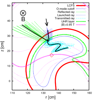
Figure 3: Ray tracing with 121 rays (only 21 rays are represented). The beam transmission efficiency is around 90%. The black solid lines correspond to the central trajectories of the launched, transmitted and reflected rays (see legend).

Figure 3 shows the result of a typical ray tracing simulation. The electron density and a temperature profiles used are fitted to the Thomson Scattering (TS) ones obtained in NBI-heated TJ-II plasmas. To calculate the electron Bernstein emission, the radiative transfer equation [18] is solved along the trajectory of the O–X transmitted rays. The solution to this equation provides the emission intensity per unit frequency, which is given by the well-known expression

$$I_{\omega}=\frac{\omega^{2}}{8\pi^{3}c^{2}}\int_{0}^{\tau(B)}T_{e}(\tau)e^{-\tau}\text{d}\tau$$ (1)

where $T_{e}$ is expressed in energy units, $c$ is the speed of light, $\omega=2\pi f$ is the wave angular frequency and $\text{d}\tau=-\alpha_{\omega}d\sigma$ is the optical thickness, with $\alpha_{\omega}$ the absorption coefficient and $\sigma$ the ray coordinate. For each transmitted ray, the integral in eq. 1 is performed along the ray path up to the inner boundary of the conversion layer, i.e. the SX–mode cut–off, in order to obtain the emission intensity $I_{i}$ prior to the single ray X–O tunneling process. Taking into account the conversion efficiency for each particular ray, $\eta_{i}$, and the Gaussian beam profile weighting factor $g_{i}$, we may write the total emission intensity as

$$I_{\text{\tiny{EBE}}}=\sum_{i}^{n_{c}}\eta_{i}g_{i}I_{i}$$ (2)

where $i$ is the ray index and $n_{c}$ is the total number of converted rays.

3.1 Dependence on mirror position, density and temperature

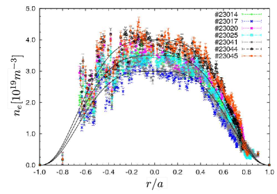
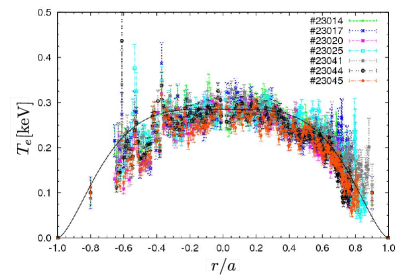
Figure 4: Experimental electron density (a) and temperature (b) Thomson scattering profiles obtained in NBI heated plasmas. The numerical calculations have been carried out using a fit to the average shape of these profiles.

In order to compare with the result of the experiments presented in section 4, the EBE calculations have been carried out for different lines of sight. The experimental TS profiles have been fitted to the functions $n_{e}(\rho)=n_{0}(1-\rho^{2n_{1}})^{n_{2}}$ and $T_{e}(\rho)=T_{0}(1-\rho^{2t_{1}})^{t_{2}}$, where the set of parameters $\{n_{1},n_{2},t_{1},t_{2}\}=\{1.6,2.7,2.0,1.7\}$ is found to match best the whole set of experimental profiles. A wide range of the $n_{0}$ and $T_{0}$ values have been considered. Figure 4 shows some of the experimental and analytical electron density (a) and temperature (b) profiles. The dependence of the electron Bernstein emission on the mirror positioning angles is plotted in the figures 5 for a fixed central density and four different values of central temperature $T_{0}$. As expected, the emission intensity increases with the electron temperature. In all cases, the maximum emission is located around $\alpha_{\phi}\approx 31^{\circ}$ and $\alpha_{\theta}\approx 21.5^{\circ}$.

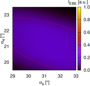
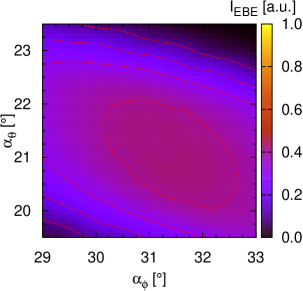
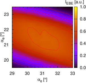
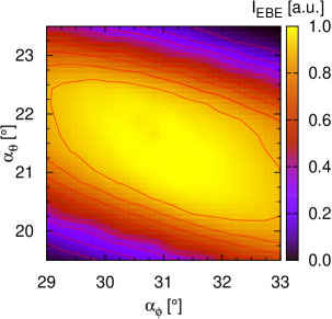
(a)  (b)  (c)  (d)

Figure 5: Dependence of the 28 GHz B–X–O mode converted radiation intensity for (a) $T_{0}=0.1$, (b) $T_{0}=0.3$, (c) $T_{0}=0.5$ and (d) $T_{0}=0.7$ KeV. In all the cases, a central density given by $n_{0}=3.5\times 10^{19}$ m^-3 has been used. Each map represents the result obtained with 256 launched beams and 121 rays per beam.

It is observed that the emission finds a stronger dependence on $\alpha_{\theta}$ than on $\alpha_{\phi}$. This is due to the more pronounced curvature of the plasma along the poloidal direction. On the one hand, this makes the incidence direction at the conversion layer deviate more sensitively from its optimum $\alpha_{\theta}$ value than from the $\alpha_{\phi}$ one, which affects to the conversion efficiency. And on the other hand, it changes appreciably the optical path of the rays and consequently the radiation reached at the O cut–off layer previous to conversion.

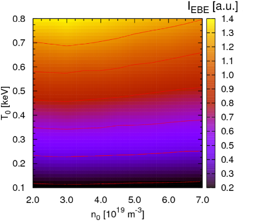
Figure 6: Dependence of the B–X–0 radiation intensity on $n_{0}$ and $T_{0}$ for the line $(\alpha_{\phi},\alpha_{\theta})=(31^{\circ},21.5^{\circ})$.

Regarding the dependence of EBE on central density, note that, as $n_{0}$ increases, the O–mode cut-off layer moves radially outwards. This modifies the O–X conversion efficiency [19] through its dependence on the values at the O mode cut-off of the characteristic density gradient scale length ($L_{n}=n_{e}/|\nabla n_{e}|$), $N_{\|}$ and $N_{\bot}$, and the magnetic field strength $B$. The final combination of these effects is illustrated in figure 6, where, independently of the central temperature $T_{0}$, a maximum intensity is observed always around $n_{0}=3\times 10^{19}$ m^-3.

3.2 Dependence on the rotation angle $\zeta$

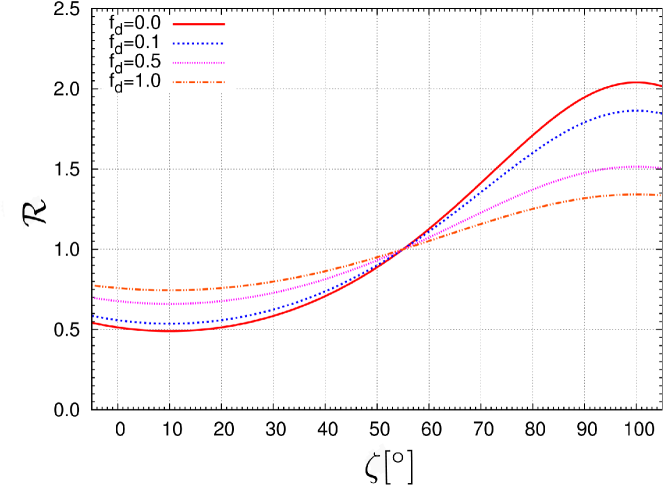
Figure 7: Dependence on the power ratio $\mathcal{R}(\zeta)$ on the EBE diagnostic rotation angle. Different non-polarized background radiation fractions are considered

.

By rotating the diagnostic we should be able to determine if there is a dominant polarization in the incoming radiation and if this coincides with the expected one. For the ideal case of a perfect elliptically polarized wave coming from the B–X–O emission, the power dissipated along each detection direction when the diagnostic rotation angle is set to some arbitrary $\zeta$ is given by eqs. 8 of the Appendix. In order to consider the presence of an unknown amount of non-polarized radiation we define

$$\mathcal{R}(\zeta)\equiv\frac{P_{1}(\zeta)+P_{d}}{P_{2}(\zeta)+P_{d}}$$ (3)

where $P_{d}\equiv f_{d}P_{2}(\zeta=10^{\circ})$ is taken as a fraction of the maximum amplitude measured in channel 2. A minimum in $\mathcal{R}(\zeta)$ is expected for $\zeta=10^{\circ}$, when channel 2 is directed along the major axis of the polarization ellipse. The dependence of $\mathcal{R}$ on the rotation angle $\zeta$ of the horn antenna is represented in figure 7 for different values of $f_{d}$. As it is clear, the greater the amount of unpolarized radiation, the flatter the $\mathcal{R}(\zeta)$ profile becomes.

4 Experimental results

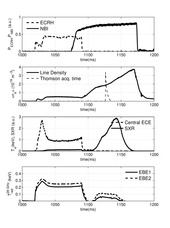
Figure 8: Typical time evolution of some relevant quantities obtained in ECRH+NBI heated plasmas.

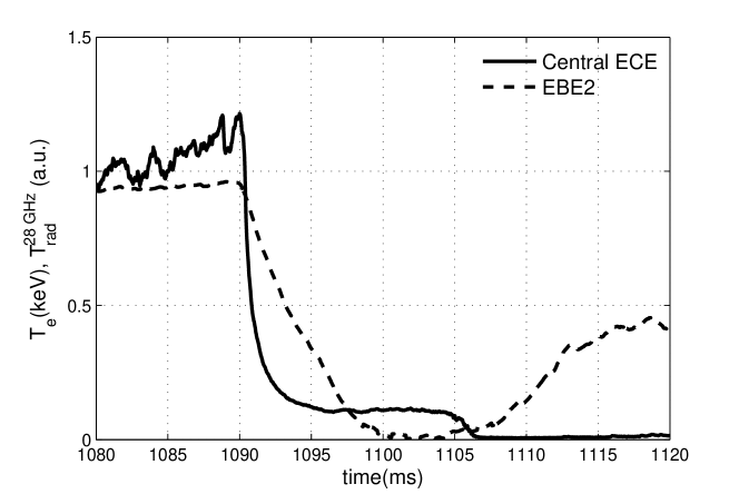
Figure 9: Zoom view of the central ECE and EBE2 signals represented in figure 8.

Figure 8 shows the time evolution of the main plasma parameters observed during a typical ECRH+NBI shot. Plasma heating is first performed by applying 500 kW of second harmonic off-axis ECRH power. Then, NBI heating ($P_{\text{\tiny{NBI}}}\approx$ 1 MW) is turned on and densities in the range $2-3.5\times 10^{19}$ m^-3 are achieved. ECRH power is turned off before the second harmonic cut-off density for 53.2 GHz ($n_{e}\approx 1.7\times 10^{19}$ m^-3) is attained. This provokes the drop in the ECE signals, which still show a low plasma temperature until the NBI-induced electron density growth prevents the detection by ECE means. The increase in the electron temperature and density during the NBI phase is accompanied with the subsequent raise of radiation observed by the Soft X ray (SXR) detector. EBE and ECE radiation after the ECRH turn-off are compared in figure 9. The ECE signal decreases faster because this diagnostic is looking to the plasma along a perpendicular line of sight whereas the EBE diagnostic is looking with a highly oblique view. Thus, the 28 GHz emission comes from suprathermal electrons with a lower collisionality than that of the thermal electrons responsible of the emission detected by the ECE diagnostic.

4.1 Experimental $\alpha_{\phi}$ and $\alpha_{\theta}$ scans

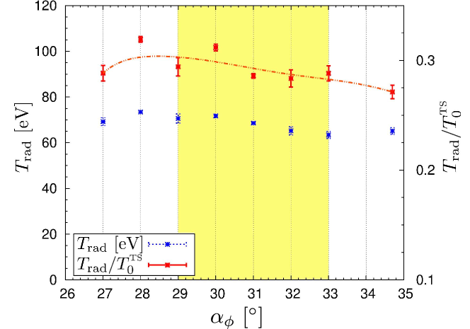
Figure 10: Dependence of $T_{\text{rad}}$ on $\alpha_{\phi}$ for $\alpha_{\theta}=21.5^{\circ}$. The shadowed area represent the interval considered in the theoretical emission plots.

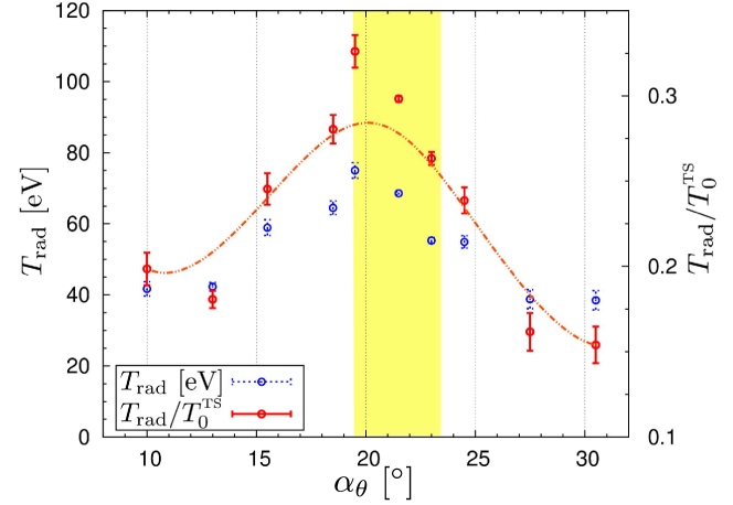
Figure 11: Dependence of $T_{\text{rad}}$ on $\alpha_{\theta}$ for $\alpha_{\phi}=31^{\circ}$.

Figures 10 and 11 show the measured radiative temperature at the TS acquisition time for different positioning angles of the internal mirror. The first of them corresponds to a scan in $\alpha_{\phi}$ for $\alpha_{\theta}=21.5^{\circ}$, while the second one represents, for $\alpha_{\phi}=31^{\circ}$, the scan in $\alpha_{\theta}$. In both figures $T_{\text{\tiny{rad}}}$ is referred to the left axis (blue dots). In order to remove its strong dependence on the temperature profile, which was not constant between shots, these values are normalized to the central temperature value ($T_{0}^{\text{\tiny{TS}}}$) provided by the TS diagnostic (red dots, right axis).

The scanned positions cover a wider area than the one considered in the theoretical calculations. The result presented in figure 10 is consistent with the theoretical predictions. The measured intensity show an almost flat profile weakly dependent on $\alpha_{\phi}$. Regarding the scan shown in figure 11 a stronger variation of the collected 28 GHz intensity on $\alpha_{\theta}$ is clearly manifested, as was also expected. The value for which a maximum emission value is obtained is $\alpha_{\theta}\approx 19.5^{\circ}$. This can be interpreted as an acceptable result compared with the theoretical prediction ($\alpha_{\theta}\approx 21.5^{\circ}$), considering that the range of movement of the mirror along the poloidal direction is $30^{\circ}$ approximately. On the other hand this disagreement of approximately $2^{\circ}$ represents a noticeable deviation compared with the width of the EBE window along the poloidal direction, which has $4^{\circ}$ (see figures 5). Furthermore, if all the radiation received came only from B–X–O-converted one, the intensity should drop drastically out of the $4^{\circ}$ of width of the viewing window. Since this is not what happens, it can be concluded that the amount of $28$ GHz disperse radiation collected by the mirror is far from being negligible. Such a contribution of disperse radiation is probably coming from EBE emitted by the over dense plasma core all around the torus. This radiation leaves the plasma via B–X–O or B–X conversion and reaches the antenna after reflecting on the walls, which also provoke randomly changes on its polarization.

4.2 Experimental determination of polarization

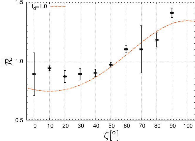
Figure 12: Experimental ratio $\mathcal{R}(\zeta)=I_{\text{\tiny{EBE1}}}/I_{\text{\tiny{EBE2}}}$ compared to the theoretical estimation, for $f_{d}=1$. A significant fraction of disperse radiation is found.

A scan of the rotation angle of the diagnostic has been carried out in order to verify that the radiation reaching the mirror contains a direct contribution of O-mode polarized radiation. If this contribution exists, we should observe a similar trend in the experimental and the theoretical ratio $\mathcal{R}(\zeta)$ (see fig. 7). The polarization has been measured along the line of sight of the mirror for which the measured EBE intensity is maximum along the poloidal angle (see fig. 11). This line of sight corresponds to the values $\alpha_{\theta}=19.5^{\circ}$ and $\alpha_{\phi}=31^{\circ}$. The rotation angle $\zeta$ was varied from $-10^{\circ}$ to $90^{\circ}$. Figure 12 shows the experimental ratio $\mathcal{R}(\zeta)=I_{\text{\tiny{EBE1}}}(\zeta)/I_{\text{\tiny{EBE2}}}(\zeta)$ measured at the TS acquisition time and the calculated one when $f_{d}=1$, that is, the value for which the best agreement is observed. Taking also into account the result shown in fig. 11, it can be concluded that the background unpolarized field contributing to the measured intensity is of the same order of magnitude of the O-mode radiation reaching the detector.

5 Summary and discussion

In this work a comprehensive study of the 28 GHz radiation rising from B–X–O conversion in over-dense TJ–II NBI-heated plasmas has been undertaken theoretically and experimentally. The numerical results have been obtained with the TRUBA ray tracing code. As expected from an X–O conversion process, highly dependent on the wave propagation direction, a strong variation of the intensity has been found as the viewing angle along the poloidal direction is modified. It has been observed that the experimental maximum of the emitted radiation was shifted $1.5-2.0$ degrees with respect to the numerical estimations, which is not negligible compared with the approximately 4 degrees of width of the EBE window along the poloidal direction. As a task for a forthcoming work, a fine scan on this angle should be performed in order to resolve that maximum. Regarding the maximum value of $I_{\text{\tiny{EBE}}}$ along the toroidal direction, the observation is in agreement with the theoretical prediction, since both theory and experiment shows an almost flat profile $I_{\text{\tiny{EBE}}}(\alpha_{\phi})$. From these results, an optimum experimental direction for forthcoming EBW heating experiments is extracted.

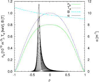
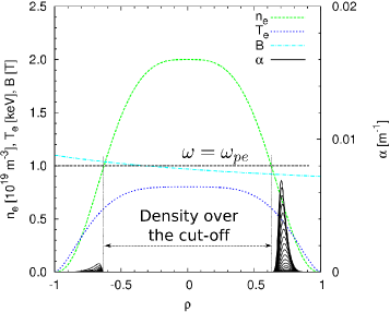
(a)  (b)

Figure 13: (a) Absorption coefficient (solid lines) for oblique O-mode propagation at $28$ GHz as a function of the effective radius, considering a cylindrical plasma with the magnetic field profile similar to the TJ-II one. The electron temperature (dashed line) and density (dotted line) profiles like those generated in ECRH-heated TJ-II plasmas are also represented. The density is under the O-mode cut-off in all the profile. (b) Oblique O–mode absorption coefficient for the over-dense case, i.e. profiles from NBI-heated TJ-II plasmas are considered. In both cases the different values of $N_{\|}$ considered are in the range between $N_{\|}\approx 0$ and $N_{\|}\approx 0.65$. The more peaked curves of the absorption coefficient correspond to the lower value of $N_{\|}$.

The polarization of the collected radiation has been measured in order to verify that the received radiation comes mainly from a B–X–O conversion process. The experiment has confirmed the existence of the expected O-mode component, importantly screened by disperse radiation.

Further discussion can be made on the possibility that this O-mode could be emitted from the under-dense plasma edge. This point is clarified in figs. 13(a) and 13(b), which show the O-mode absorption coefficient for different values of $N_{\|}$ in a cylindrical plasma with typical TJ–II magnetic field, electron density and temperature profiles. This has been estimated by using well-known expressions of the weakly relativistic absorption coefficient of electromagnetic modes [20]. On the one hand, figure 13(a) represents the case where the density is below the O-mode cut-off, i.e. between 1025 and 1100 ms in figure 8. On the other hand, figure 13(b) shows the over-dense case in the interval between 1100 and 1150 ms. The absorption coefficient in the over-dense scenario is three orders of magnitude lower than in the under-dense case. Since in this situation the absorption of the O-mode is negligible in the edge, so is the emission coefficient. This allows to conclude that the O mode polarized radiation measured when in over-dense conditions can only be attributed to a B–X–O process.

A considerable amount of disperse radiation has been found. Its presence can be understood by considering that the emission of EBWs takes place all around the over-dense plasma column and reaches the antenna after many reflections in the vacuum chamber, which in turn produces a random polarization. Further studies on the characterization of the disperse radiation using ray tracing are planned. This task results extremely important due to the role of this contribution to the deterioration of the EBE signal. As a matter of fact, the disperse radiation together with the presence of the X–O conversion layer in between the emitting source and the radiometer horns, represents a handicap in the calibration of the EBE signal by traditional means if the electron temperature diagnosis in over-dense regime is aimed. Note that X–O conversion layer act as a kind of $\mathbf{k}$-spectrum filter that can not be taken into account in the calibration procedure. It could only be included a posteriori knowing the exact O–X conversion efficiency of the beam and assuming a symmetric conversion efficiency, which is not always true. Moreover, as it was briefly mentioned in section 3, the calculation of the beam O-X conversion efficiency by ray tracing is not accurate, making the final determination of an electron temperature a very hard task.

Finally, the improvement in the spatial resolution by considering a more collimated viewing pattern as in standard ECE measurements could help to get rid of the disperse radiation. However, this will be accompanied by a X–O conversion efficiency drop due to the widening of the $\mathbf{k}$-spectrum of the field associated to a highly collimated beam and, consequently, the EBE source for the temperature measurement would be strongly screened by the disperse radiation.

Appendix: Expected power for an arbitrary rotation angle

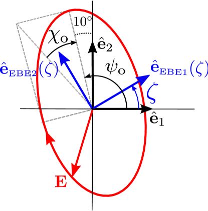
Figure 14: Theoretical O-mode polarization ellipse. In the figure, the azimuth is defined in the non rotated frame ($\zeta=0$). The polarizations vectors of the detector when it is rotated an angle $\zeta$, $\hat{\mathbf{e}}_{\text{\tiny{EBE1}}}(\zeta)$ and $\hat{\mathbf{e}}_{\text{\tiny{EBE2}}}(\zeta)$, are also represented.

For the derivation of an explicit form of the powers $P_{1}(\zeta)$ and $P_{2}(\zeta)$, the ideal theoretical polarization of the B–X–O radiation is first defined in the main reference system given by the polarization vectors $\hat{\mathbf{e}}_{1}$ and $\hat{\mathbf{e}}_{2}$ (see figure 14). As already anticipated, the azimuth of the O mode polarization ellipse in this reference system can be obtained from geometrical calculations by finding the projection of the $\{\mathbf{k},\mathbf{B}\}$ plane, defined at the plasma boundary, onto the detection plane of the horn, after the two successive reflections both in the elliptical and the flat mirror. Furthermore, in order to couple an obliquely propagating ordinary mode at the plasma edge the wave must be elliptically polarized with an ellipticity angle $\gamma$ given by

$$\tan{\gamma}=\frac{Y(\sin^{2}\theta-\varrho)}{2\cos\theta},$$ (4)

where $\varrho^{2}\equiv\sin^{4}\theta+(4/Y^{2})\cos^{2}\theta$, $Y=\omega_{ce}/\omega$ and $\theta$ is the propagation angle at the plasma edge. For the standard TJ–II magnetic configuration and taking into account the fact that the detector is looking to the emitted wave (the rotation sense of the electric field is reversed), we finally obtain the angles that define the polarization ellipse in the main reference system, i.e.

$$\psi_{\text{\tiny{O}}}=100^{\circ},\ \ \ \chi_{\text{\tiny{O}}}\equiv-\gamma=-35^{\circ}.$$ (5)

Taking $|E_{1}|^{2}+|E_{2}|^{2}\equiv 1$ the relation between these angles and the wave electric field is given by [21]

$$\begin{split}&s_{1}=E_{1}^{2}-E_{2}^{2}=\cos 2\chi_{\text{\tiny{O}}}\cos 2\psi_{\text{\tiny{O}}},\\ &s_{2}=2|E_{1}||E_{2}|\cos\delta=\cos 2\chi_{\text{\tiny{O}}}\sin 2\psi_{\text{\tiny{O}}},\\ &s_{3}=2|E_{1}||E_{2}|\sin\delta=\sin 2\chi_{\text{\tiny{O}}},\end{split}$$ (6)

where $|E_{1}|$, $|E_{2}|$ and $\delta\equiv\delta_{2}-\delta_{1}$ determine the complex electric field amplitude through $\mathbf{E}=E_{1}\hat{\mathbf{e}}_{1}+E_{2}\hat{\mathbf{e}}_{2}=|E_{1}|\exp(\text{i}\delta_{1})\hat{\mathbf{e}}_{1}+|E_{2}|\exp(\text{i}\delta_{2})\hat{\mathbf{e}}_{2}$. Consider now the field components in an arbitrary $\zeta-$rotated system defined by the two orthogonal directions of the EBE diagnostic: $\mathbf{E}=E^{\prime}_{1}\hat{\mathbf{e}}_{\text{\tiny{EBE1}}}+E^{\prime}_{2}\hat{\mathbf{e}}_{\text{\tiny{EBE2}}}$.Note that when $\zeta\approx 10^{\circ}$, the vector $\hat{\mathbf{e}}_{\text{\tiny{EBE2}}}$ is directed along the major axis of the polarization ellipse. Therefore, the power detected in both channels, for an arbitrary angle $\zeta$, is given by

$$\begin{split}&P_{1}(\zeta)=E^{\prime}_{1}{E^{\prime}_{1}}^{*}=|E_{1}|^{2}\cos^{2}\zeta+|E_{2}|^{2}\sin^{2}\zeta+2\Re(E_{1}E_{2})\cos\zeta\sin\zeta\\ &P_{2}(\zeta)=E^{\prime}_{2}{E^{\prime}_{2}}^{*}=|E_{2}|^{2}\cos^{2}\zeta+|E_{1}|^{2}\sin^{2}\zeta-2\Re(E_{1}E_{2})\cos\zeta\sin\zeta.\end{split}$$ (7)

Recovering the relations (6) and taking $\delta_{1}=0$, $P_{1}$ and $P_{2}$ can be written as

$$\begin{split}&P_{1}(\zeta)=\left(\frac{1+s_{1}}{2}\right)\cos^{2}\zeta+\left(\frac{1-s_{1}}{2}\right)\sin^{2}\zeta+s_{2}\cos\zeta\sin\zeta\\ &P_{2}(\zeta)=\left(\frac{1-s_{1}}{2}\right)\cos^{2}\zeta+\left(\frac{1+s_{1}}{2}\right)\sin^{2}\zeta-s_{2}\cos\zeta\sin\zeta.\end{split}$$ (8)

For $\zeta=10^{\circ}$, $P_{2}$ is maximum.

References

- [1] Bernstein I B 1958 Phys. Rev. 109 1 10
- [2] Mueck A et al2007 Phys. Rev. Lett. 98 175004
- [3] Laqua H P et al1999 Plasma Phys. and Contr. Fusion 41 A273-A284
- [4] Igami H et al2009 Nucl. Fusion 49 115005
- [5] Preinhaelter et al2009 Plasma Phys. and Contr. Fusion 51 125008
- [6] Laqua H P 2007 Plasma Phys. and Contr. Fusion 41 R1-R42
- [7] Volpe F, Laqua H P and the W7-AS Team 2003 Rev. Sci. Instrum. 74 3 1409
- [8] Jones B et al2004 Phys. Plasmas. 11 3, 1028
- [9] Alejaldre C et al1990 Fusion Technology 17 131
- [10] Castejón F et al2006 Fusion Science and Technol. 52 2 230
- [11] Curto A F et al2005 Fusion Eng. and Design 74 325
- [12] Castejón F et al2008 Nucl. Fusion 48 7 075011
- [13] Caughman J B O 2006 et alProc. 14th Joint Workshop ECE and ECRH p. 243
- [14] Caughman J B O 2010 et alFusion Science and Technol. 57 1 41
- [15] Tereshchenko M A et al 2003 Proceedings of the 30th EPS Conference on Contr. Fusion and Plasma Phys. 27A P-1.18
- [16] Tribaldos V, van Milligen B P and López-Fraguas A L 2001 Informes Técnicos del Ciemat 963
- [17] Köhn A et al 2008 Plasma Phys. and Contr. Fusion 50 085018
- [18] Bekefi G 1966 Radiation Processes in Plasmas (Wiley N.Y.)
- [19] Mjølhus E J 1984 J. Plasma Phys. 31 7
- [20] Bornatici M et al1983 Nucl. Fusion 23 9 1153
- [21] Chandrasekhar M 1950 Radiative Transfer (Oxford Press)