arXiv:1008.4769
Limits on the Time Variation of the Fermi Constant Based on Type Ia Supernova Observations
Alejandro Ferrero and Brett Altschul
Department of Physics and Astronomy
University of South Carolina
Columbia, SC 29208 USA
Abstract
The light curve of a type Ia supernova decays at a rate set by the -decay lifetimes of the 56Ni and 56Co produced in the explosion. This makes such a light curve sensitive to the value of the Fermi constant at the time of the supernova. Using data from the CfA Supernova Archive, we measure the dependence of the light curve decay rate on redshift and place a bound on the time variation of of yr-1.
1 Introduction
Finding new fundamental physics beyond the standard model and general relativity has long been a topic of great interest. One way to identify definitive evidence of new physics is to look for exotic phenomena that simply cannot occur in the standard physical theories. One such exotic possibility that has provoked significant interest is having time-dependent fundamental constants [1, 2, 3, 4, 5, 6, 7, 8].
The possibility of time-varying fundamental constants opens up many new lines of inquiry. The most commonly studied theory with varying constants is one with a time-dependent fine structure constant . A quantum approach to this subject can be found in [9], while other approaches treat the problem rather phenomenalistically (e.g. [10]). Another possibility that has been fairly well studied is a change in the quantum chromodynamics scale and therefore the electron-proton mass ratio.
If some of the fundamental constants in nature are allowed to change over time, the effects of these changes might be detected. Searches for such temporal variations entail measurements of the same experimental observable at different points in time, to see if there is any change. However, since the changes involved should be tiny, laboratory experiments searching for them demand very high precision. Less precision is required if large time scales are involved; a very slow time variation can be observed if the times used to detect it are long enough. Thus, cosmological observations, which give us a view of how physics operated millions or billions of years in the past, seem to be good candidates to test for time variations in fundamental constants.
The purpose of this paper is to study a possible change in the Fermi constant . This quantity is defined to be , with the standard model’s gauge coupling constant and the mass of the boson. Since the vector boson mass is , is really a measure of , the Higgs field vacuum expectation value. The masses of fundamental fermions depend on and the values of the fermion-Higgs Yukawa couplings , with . So a changing value of would also affect the fermion masses unless the couplings also changed to compensate. Since there is no evidence of any time variation in in atomic spectra, we shall assume that such cancellation between the time variation of and occurs, even though that is not a particularly natural scenario.
also governs the strength of charged current weak interactions at low energies. It can be measured with relatively high precision by studying the lifetimes of muons, and its accepted value is GeV-2 [11, 12]. However, laboratory measurements of decay rates are not precise enough to offer a particularly promising way of measuring . On the other hand, the light coming from supernovae explosions can provide a useful way to study weak interactions that occurred at much earlier times.
In Section 2, we shall discuss the physics of supernovae and how their light curves are related to the Fermi coupling constant . Section 3 covers the details of the calculational methodology used to relate the supernova light curve data to . In Section 4, we apply this methodology to data from the Harvard-Smithsonian Center for Astrophysics (CfA) Supernova Archive [14, 15] and state our results. Section 5 presents conclusions and outlook.
2 Supernova Structure
Supernovae are catastrophic variable stars that, having previously produced energy through steady-state fusion processes, explode and release huge additional amounts of energy. The amount of energy released is so vast that even cosmologically distant supernovae can be easily detected in the sky. Normal stars avoid gravitational collapse because nuclear fusion processes are constantly generating energy in their cores, where the high temperature and pressure enable light nuclei to overcome their electrostatic repulsion and fuse. A large red giant star may burn a significant portion of its mass into isotopes of iron, beyond which further fusion is no longer exothermic. However, smaller stars, without thick external layers to compress the core to the high temperatures and pressures needed to produce iron, may cease burning when the core is mostly carbon and oxygen, without having extracted all of this fuel’s available energy. In either case, the core of the star settles down to become a white dwarf, supported against gravitational collapse by the degeneracy pressure of its electrons.
If the mass of a white dwarf star is larger than approximately (the Chandrasekhar mass ), the electron degeneracy pressure can support the star against gravitational collapse. However, if the mass of the star grows larger than this limit, the electron pressure can no longer prevent a collapse. Such a collapse triggers the release of a tremendous amount of energy and the star becomes a supernova. Iron white dwarfs at the cores of massive stars collapse to form even more compact objects—neutron stars or black holes. However, of interest here are the type Ia supernovae produced from carbon-oxygen white dwarfs. These stars may accrete mass from (or possibly merge with) their partners in binary systems, until the white dwarf’s mass becomes sufficient to trigger a supernova. When these stars exceed , they begin to collapse. However, the collapse phase is short-lived; as the star contracts, there is an increase in temperature and density in the core of the star, which allows the ignition of carbon fusion. Within a short period of time, a huge amount of fusion energy is released, blowing the star apart and increasing its luminosity to enormous values. (The total luminosity may be that of millions of ordinary suns).
In this paper, we shall be analyzing the light curves of type Ia supernovae. The near equality of the masses of the white dwarf progenitors gives them all similar energy outputs and makes them extremely important standard candles in cosmology. Type Ia supernovae all seem to follow a characteristic light curve. (Some corrections to the light curves are required in order for the population of type Ia supernovae to act as genuinely standard candles, but these are not important for our present purposes.) The relative uniformity of this curve structure for different stars also makes them a very useful tool for studying certain physical properties.
The light curve is a plot of the apparent magnitude of the source versus time; is the radiation flux from the source, and is a reference value of the flux defining 0 magnitude. Using different kinds of filters, which cover different parts of the spectrum, several different magnitudes may be measured for a single source. There is a separate light curve for each band, but the curves for different colors show similar behavior, which is again consistent across different sources.
At early times, the brightness of a supernova increases rapidly until it reaches a maximum, which is followed by two regions in which decreases linearly (corresponding to exponential decays in the flux). Since type Ia supernovae are ultimately powered by uncontrolled nuclear fusion, they produce large quantities of the heavy elements, especially those elements with binding energies close to the maximum value. Specifically, each supernova produces a great deal of the double magic nucleus 56Ni. This nucleus decays by electron capture (EC) to 56Co with a lifetime of 6.077 d, and this decay provides much of the energy released by the supernova during its earlier stages. The first linear region along the light curve corresponds to the period during which 56Ni decay is the dominant source of heating. The daughter nucleus 56Co also decays by EC to 56Fe, with a lifetime of 77.27 d. At later times (in the second, more slowly decaying linear region), it is this decay that primarily fuels the supernova’s luminosity. This region, whose extent is determined by the decay rates of 56Ni and 56Co, can be found between approximately 35 and 100 days after the maximum magnitude is reached. During this time, some months after a supernova reaches its peak, the light curve approximately tracks the quantity of 56Co still present. The falloff in the luminosity can therefore be used to measure the lifetime of this nuclide at the time the supernova occurred. This gives direct information about the value of several standard model parameters at the time of the explosion’s occurrence, including . This was first suggested in [13], when much less data was available.
An EC decay rate depends on fundamental constants in the following fashion. Being a tree-level weak decay, the rate is naturally proportional to . However, it also depends on the probability that an -state electron will be found close enough to the nucleus to be taken up by a proton. The nuclear volume is proportional to . The square of the electron wave function in the vicinity of the nucleus is proportional to , where is the Bohr radius. The inverse of the mean life of a nucleus that is unstable against EC is therefore proportional to the combination of fundamental quantities . (The rate also depends on the -value of the decay, which is further dependent on and , in more complicated fashion.) However, changes in and are much easier to measure than would be changes in . and affect atomic energy levels directly, so their time derivatives can be constrained by comparing spectra taken at different times. Cosmological and laboratory measurements have constrained these dimensionless quantities to vary only by parts in or less per year.
A supernova’s light curve and total luminosity are also affected by the value of the gravitational constant . The amount of 56Ni produced in the explosion is proportional to the total mass of the collapsing star, [16, 17]. Observations of supernovae have been used to place bounds on the variation of at the yr-1 level. We choose here to look at a model that neglects variations in , although an analysis that considered simultaneously varying and would also be interesting. We shall also neglect any possible time dependences of and , in light of the strong bounds on such time dependences. This means there is a simple relationship between and ,
| (1) |
Bounds on changes in the 56Co decay rate may thus be interpreted as bounds on a change in the Fermi constant.
3 Method
In the light curve of a type Ia supernova, the slope of the second linear region is related to the decay rate of 56Co. The main goal of this paper is to compare this slope across different supernovae of different ages. The slope for each one is related to the Fermi constant at a particular time. We will make this comparison using data from the CfA Supernova Archive.
Ideally, one could simply measure the slopes of the supernova light curves in their 56Co-dominated regions and then determine whether the slopes are correlated with the ages of the events. However, several corrections must be made before this can be done.
The light curves do not give a pure measurement of the 56Co lifetime; what is observed is the luminosity of the supernova remnant. The EC decay is the object’s main energy source, but the decay energy is moderated through the complicated interactions of the expanding gas, so the luminosity does not track perfectly with the 56Co decay profile. The details of the remnant dynamics differ a bit from supernova to supernova. It is not possible to correct for this lack of complete uniformity in the structures, and this will necessarily be a source of random error.
Some of the corrections may be handled more simply, however. This is the case for the correction arising from the well-known Doppler shift associated with the expansion of the Universe. Since the inverse of the mean life, , measures how fast 56Co is decaying (and therefore, the frequency at which EC processes are occurring), the observed value of will be subject to the same cosmological redshift as any other frequency. In terms of the red shift , the measured value on Earth and the proper decay rate at the exploding star are related by
| (2) |
The physical effect of the redshift is to slow down the decay of the light curve.
We shall denote by the slope of the second linear region of each particular light curve, as observed on the Earth. This slope and the 56Co decay rate should be directly proportional, so we have
| (3) |
where is the proper decay rate of the supernova light curve, and is a proportionality constant related to the complex physics of the explosion. The quantity is proportional to the square of the Fermi coupling constant at the time that the explosion occurred, . If has changed over time, we would expect to see a change in the decay rates observed for different supernovae. Comparing the light curves for supernovae of different ages gives a good way to measure a change in the Fermi coupling constant.
The light from a particular supernova is emitted and collected at the times and , respectively. Denoting the scale factor of the Universe by and the Hubble constant by , we have the standard relations
| (4) | |||||
| (5) |
The factor converts derivatives with respect to into ones with respect to time. Based solely on the relations (4) and (5), one may be tempted to conclude that (where is the average value of as computed from the different sources). However, a new complication arises because of the differences in the behaviors of the observed in different wavelength bands, and this relation for is subject to further corrections. Looking at the light from different color regions, we see slightly different slopes associated with the different bands. At first glance this might not seem to be a problem, since the value of the proportionality constant defined in eq. (3) could just be redefined for each band. The value does not depend on , so it would not affect the final result.
Nevertheless, the fact that does not remain constant across the various bands introduces a new correction. To understand why a further correction is necessary, let us consider light that is detected on Earth using a red filter. This light has been redshifted by the expansion of the Universe. If the slopes for the different bands were the same this would not be a problem, but the red light that is detected actually had a shorter wavelength when it was emitted during the explosion. All the red light that is detected on Earth was some amount bluer at the time of its emission; and we should ideally be comparing light from different sources that had the same wavelength at the time of emission—not at the time of observation. If the light curve steepens with increasing wavevector , the redshift would transform this into a steepening (within a given wavelength band) as a function of , because the older light originally had a higher frequency. What is required is similar to a light curve correction [18]. However, rather than using tabulated corrections, we shall, for this low redshift sample of supernovae, calculate our correction directly from the data set. This is justified because the technique minimizes our reliance on the results of unrelated fits and because we shall find that the correction it produces is relatively small.
To account for the redshift’s effect, we suppose that the dependence of on is weak, and make a linear approximation
| (6) |
is the observed slope in the band with mean wavenumber . Once corrected by , gives the proper decay rate , but for a band centered at a higher wavenumber . The dependence of generates a spurious dependence on in the observational data, which we must subtract away.
Unlike the simple factor relating to (which is an exact correction), there is no particular reason for this effect to be linear in . The wavelength dependence of the proportionality constant is a consequence of the complicated dynamics of the supernova remnants; its detailed form is not known. If is itself a function of , there will be corrections to (6). At the same order, it would also be necessary to correct the average to account for the fact that we are actually averaging decay rates in different color regions. We are neglecting these possibilities (which would correspond to corrections that are higher order in in our final formula for ), because the redshifts in the sample we shall study range only from to . However, these corrections can be computed, and working with sources at higher would require us to have a better knowledge of how depends on . Yet there is a limit to the precision that can be derived from more detailed models, since there are data available for only a handful of wavelength bands (five in this case), and data points at multiple frequencies would be required to map out the detailed dependence of on .
In principle, we could try to correct the values of for each supernova individually, by studying the dependence of its light curves on . We could then use the corrected values obtained separated for each source to compute . However, this would require additional fitting for each supernova, which may introduce additional errors and which cannot be practically implemented for many of the sources because of the limited data available. We shall therefore make only a single calculation of , using the combined data from all the sources.
Using eq. (6) we find our final formula for ,
| (7) |
including the linear correction to eliminate the spurious dependence caused by a nonzero . Evaluating this requires multiple fits. The order of the fitting procedures is as follows. First, is determined for each supernova in each band separately. These are then fitted as a linear function of the redshift , giving both an average and a slope for each band. From the fit of the five average values versus , the parameter can be extracted. Then can be evaluated according to eq. (6); this evaluation can be done separately in each of the five bands, although the single fitted value for the quantity is common to all of them.
The overall negative sign in eq. (7) merits some explanation. Because the light curves are decaying in the region of interest, is always negative. If is more negative at greater values of ( and , the decay rate was faster at earlier times. This means and thus are decreasing as time passes, leading to the negative sign in eq. (7).
4 Data Analysis
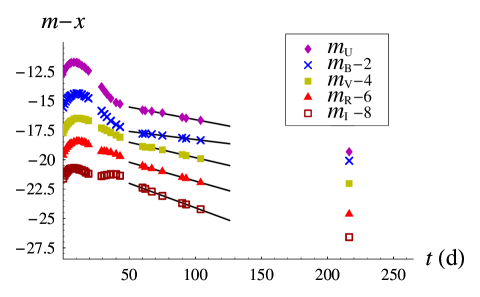
Using the method we have discussed, we can now place a bound on the time variation rate of using data from the CfA Supernova Archive. For purposes of illustration, we shall initially focus on one particular supernova, SN 1998aq [19], for which . Its light curves are shown in fig. 1, plotting the supernova’s magnitude as a function of time in days. The linear behavior arising from the 56Co decay can be seen in a region covering approximately 50–130 days after the maximum magnitude was recorded. Although the data has small errors related to the measurements, these have been omitted for clarity of presentation. To find the slopes in the different bands, we used a weighted linear fit in the region of interest, minimizing the per degree of freedom. The results of these fits are also shown in fig. 1 and the fitted slopes are listed in table 1. In order to transform these results into the reference frame of supernova, we just use the relation .
| Band | (10-4 d-1) |
|---|---|
| U | |
| B | |
| V | |
| R | |
| I |
We have applied the same procedure to multiple sources. Not all sources in the CfA Supernova Archive had sufficient data to be fitted reliably, and not all bands were represented for all sources. In table 2, we summarize the results found for the different supernovae we analyzed. The slopes are in the observer reference frame on Earth (no factor included). There was one further complication associated with fitting some of the light curves. For some sources, there is limited data at early times, and it was not possible to resolve the date at which the light curve achieved its absolute maximum. In many cases, we could identify the proper linear region by inspection, but if there was any doubt whether a given data point should be included, the fitted region was chosen so as to produce the best linear fit.
| Source | (d-1) | (d-1) | (d-1) | (d-1) | (d-1) | |
|---|---|---|---|---|---|---|
| 1995bd | – | – | – | |||
| 1998aq | ||||||
| 1994ae | – | |||||
| 1995al | – | |||||
| 1995D | – | |||||
| 1999gh | ||||||
| 2000cx | ||||||
| 1999ac | ||||||
| 1998bp | – | – | – | |||
| 1998es | – | – | ||||
| 1995E | – | – | ||||
| 1999dq | ||||||
| 1999aa | ||||||
| 1993ae | – | – | ||||
| 1994M | – | |||||
| 1995ak | – |
The data available for some supernovae and some wavelength bands were not of sufficient quality to be useful. We omitted those sources for which the standard error in the fit of was larger than 0.015 d-1 and those with fewer than three data points in the region of interest. The former was indicative of substantial deviations from linear behavior (that is, nonexponential decay in the luminosity), and the later simply represented too few points to be useful.
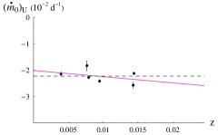
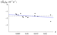
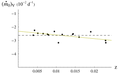
The dependence of for each wavelength band is shown in fig. 2. It is evident that is negative in each of the five distinct wavelength regimes. The values of the slopes, as well as some other relevant quantities, are collected in table 3.
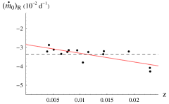
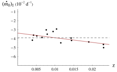
| Band | (nm) | (d-1) | (d-1) |
|---|---|---|---|
| U | |||
| B | |||
| V | |||
| R | |||
| I |
The last fit required was for the wavelength dependence of . The result was nm/d. The correction associated with this factor will make only a small contribution to the final value of . This correction, along with the other factors necessary to produce the final computed value of , are given in table 4. The fourth column of this table collects all the corrections for each band, giving the full -dependence of the 56Co decay rate ; only a factor of the Hubble constant is needed to convert this into a time dependence.
| Band | |||
|---|---|---|---|
| U | |||
| B | |||
| V | |||
| R | |||
| I |
5 Conclusions
Our main result, eq. (8), shows that the Fermi constant may be decreasing with time; however, the evidence for a change is at less than the level. The error is too large to conclude that there is any systematic change in or . Stating our results as a bound, we have
| (9) |
The main source of error was the fitting errors associated with the determination of . Nevertheless, the results for the variation of the decay rate of the 56Co isotope seem to be roughly consistent across the five different wavelength bands.
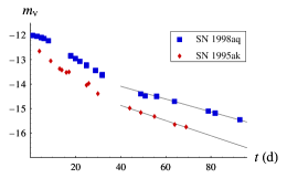
Most of the statistical pull toward a negative value of comes from two sources, SN1995ak and SN1994M, at comparatively high redshifts. The V-band light curves for SN 1995ak and the more typical SN 1998aq are shown in figure 3. The two sources at the highest values show markedly more rapid light curve decays than do the lower- supernovae. When sources such as these are used for cosmic distance scale measurements, the more rapid decay is removed by applying a stretch factor to the time axis [21]. However, the use of such an empirically determined factor appears to be inappropriate here; it could rescale away any actual signal from variations in that was seen from the data. If is not varying, some other systematic difference between these sources and the others is probably responsible, but the nature of this difference is unknown.
The second term in eq. (7), which comes from the dependence of , is considerably smaller than the first term, which accounts for its direct dependence on . Thus, the poorly understood physics that causes the light curve to depend on wavelength contributes only a small adjustment to the inferred value of . This was found to be true in all the bands. Since the leading order correction due to the -dependence is small, as is for the sources we have considered, we do not expect there would be any important changes to if higher order in corrections were taken into account. However, if sources with greater redshifts were to be analyzed, the higher order corrections would need to be considered and their contributions could be important.
More sources should be analyzed for this method to produce its best possible result for the time variation of the Fermi constant. Although the CfA Supernova Archive contained plenty of information for small redshift supernovae (), more large redshift supernovae should also be analyzed in order to obtain better results. At present, the yr-1 bound on the fractional time variation can be seen as ruling out roughly a 10% change in over about 100 million years of time. Although the late time behavior of light curves is more difficult to observe for more distant supernovae, using older sources could significantly improve these results. It would also be desirable to have more data with well-defined locations for their maxima; light curves with more data points in the linear region of interest would also be particularly valuable.
We found no significant evidence for a change in over the cosmological interval we studied, . However, if we did see a systematic shift in the decay rate of the supernova light curves, it could probably be more reasonably explained by something other than a change in the strength of the weak interaction. We have not measured (or the half-life of 56Co) directly. Changes in supernova composition over the lifetime of the sample could potentially have affected the decay rate of the light curve, changing the way the 56Co decay products heat the expanding remnant. Statistically significant evidence for systematic changes in the supernova light curves over the lifetime of the universe would be suggestive, but it would by no means be compelling evidence for changing fundamental constants.
This analysis has determined the rate of change of the dimensional quantity . In general, only the time dependence of dimensionless numbers can be defined unambiguously. A quantity with dimensions must be compared with some similarly dimensioned reference unit, which may itself depend on time in a correlated fashion; what reference is chosen will affect how the measured quantity appears to depend on time. However, there is essentially no problem in this instance. We can calculate how the dimensional parameter (or ) depends on time with no meaningful ambiguity—just as one can observe the growth in a child’s weight over time without confronting any ambiguity—since any reference with which the dimensional observable is implicitly compared is independent of . All possibly relevant time standards with which could be compared have the same dependence on —none.
In order to extend these bounds to data sets with older, more distant supernovae, we would need to account for several additional complications. For very distant sources (and especially for late periods along the light curve), the quality of the magnitude data diminishes. In addition to limiting the amount of usable data, this could introduce unexpected biases into the data. (For example, light curves with more rapid 56Co decay rates might be underrepresented in the set of usable data, because their luminosity falls below the threshold for detection more quickly, providing too few data points to map out the relevant region of their light curves accurately.) A more systematic correction would probably also be required at high redshifts, and it would be desirable to make use of more detailed models of type Ia supernovae structure, so as to get at the 56Co lifetime more directly.
These are not the first published bounds on . Although the Fermi coupling constant cannot straightforwardly be observed through its effects on atomic spectra, it does effect nuclear energy levels in a small way. Aside from astrophysical observations of ancient events and precision laboratory experiments, the most successful method for placing bounds on the time variations of fundamental constants has been to look at the isotopes produced by the natural reactors that operated near Oklo, Gabon about years ago. A bound on the fraction change in the dimensionless quantity at the yr-1 level was based on the production of samarium isotopes at Oklo [22]. However, bounds based on the Oklo data require a very detailed understanding of the operation of the reactor, as well as complicated nuclear structure calculations, whose reliability as regards the effects of is somewhat questionable. Therefore, our technique, which can be extended to older supernovae, may offer the best possibility for placing robust bounds on the time variation of the Fermi constant.
Acknowledgments
The authors wish to thank Santiago Gonzalez for his helpful comments. This research has made use of the CfA Supernova Archive, which is funded in part by the National Science Foundation through Grant No. AST 0606772.
References
- [1] M. Fischer, et al., Phys. Rev. Lett. 92, 230802 (2004).
- [2] E. Peik, B. Lipphardt, H. Schnatz, T. Schneider, Chr. Tamm, S. G. Karshenboim, Phys. Rev. Lett. 93, 170801 (2004).
- [3] P. Tzanavaris, J. K. Webb, M. T. Murphy, V. V. Flambaum, S. J. Curran, Phys. Rev. Lett. 95, 041301 (2005).
- [4] C. R. Gould, E. I. Sharapov, S. K. Lamoreaux, Phys. Rev. C 74, 024607 (2006).
- [5] A. Cingoz, A. Lapierre, A.-T. Nguyen, N. Leefer, D. Budker, S. K. Lamoreaux, J. R. Torgerson, Phys. Rev. Lett. 98, 040801 (2007).
- [6] S. Blatt, et al., Phys. Rev. Lett. 100, 140801 (2008).
- [7] M. T. Murphy, V. V. Flambaum, S. Muller, C Henkel, Science 320, 1611 (2008).
- [8] M. E. Tobar, P. Wolf, S. Bize, G. Santarelli, V. Flambaum, Phys. Rev. D 81, 022003 (2010).
- [9] A. Ferrero, B. Altschul, Phys. Rev. D 80, 125010 (2009).
- [10] V. V. Flambaum, Int. J. Mod. Phys. A 22, 4937 (2007).
- [11] D. B. Chitwood, et al. (MuLan Collaboration), Phys. Rev. Lett. 99, 032001 (2007).
- [12] A. Barczyk, et al. (FAST Collaboration), Phys. Lett. B 663, 172 (2008).
- [13] R. J. Scherrer, D. N. Spergel, Phys. Rev. D 47, 4774 (1993).
- [14] A. G. Riess, et al., Astron. J. 117, 707 (1999).
- [15] S. Jha, et al., Astron. J. 131, 527 (2006).
- [16] E. Gaztañaga, E. García-Berro, J. Isern, E. Bravo, I. Domínquez, Phys. Rev. D, 65 023506 (2001).
- [17] A. Riazuelo, J. Uzan, Phys. Rev. D, 66 023525 (2002).
- [18] E. Hubble, Astrophys. J. 84, 517 (1936).
- [19] A. G. Riess, et al., Astrophys. J. 627, 579 (2005).
- [20] A. G. Riess, et al., Astrophys. J. 699, 539 (2009).
- [21] S. Perlmutter, et al. Astrophys. J. 483, 565 (1997).
- [22] T. Damour, F. Dyson, Nucl. Phys. B 480, 37 (1996).