Penetration of hot electrons through a cold disordered wire.

Abstract

We study a penetration of an electron with high energy $E\gg T$ through strongly disordered wire of length $L\gg a$ ($a$ being the localization length). Such an electron can loose, but not gain the energy, when hopping from one localized state to another. We have found a distribution function for the transmission coefficient ${\cal T}$. The typical ${\cal T}$ remains exponentially small in $L/a$, but with the decrement, reduced compared to the case of direct elastic tunnelling: $\overline{\ln{\cal T}}\approx 0.237\cdot 2L/a$. The distribution function has a relatively strong tail in the domain of anomalously high ${\cal T}$; the average $\overline{{\cal T}}\propto(a/L)^{2}$ is controlled by rare configurations of disorder, corresponding to this tail.

The electronic transport in disordered one-dimensional systems was extensively studied in the past 50 years Anderson ; review . In the non-interacting system all the states are localized Berezinskii , so that the transmission coefficient ${\cal T}$ of a finite system exponentially decays with $L$. ${\cal T}$ varies from sample to sample, since it depends on the configuration of disorder. For strongly disordered chains the distribution of $s\equiv-(1/\alpha)\ln{\cal T}$ is a narrow gaussian:

$$F_{0}(s)\propto\exp\{-(s-1)^{2}/(\Delta s)^{2}\},\quad\Delta s=B\alpha^{-1/2},$$ (1)

$$\alpha=2L/a\gg 1,$$ (2)

being the principal large parameter of the theory (the measure of the localization strength), $B\sim 1$ being the model-dependent factor noninteracting . Thus, the conductivity of a noninteracting system is zero at $L\to\infty$.

The interactions (e.g., with phonons) lead to a finite equilibrium conductivity $\sigma$ of the hopping type (see EfrosShklovskii ). At some $L\sim L_{0}(T)$ the exponential $L$-dependence of the conductance $G$ is changed to $G=\sigma/L$, with $\sigma$, exponentially dependent on the temperature $T$ of the system. The specifics of strongly disordered 1d systems was properly taken into account in Kurkijarvi ; RaikhRuzin ; it was shown that the conductivity in the variable range hopping regime is controlled by rare fluctuations of the density of states at the fermi level – the “breaks”; as a result

$$\sigma\approx\exp\{-T_{0}/2T\},\quad T_{0}=1/ga,$$ (3)

where $g$ is the average density of states. The result (3) does not obey the Mott law $\sigma\propto\exp\{-c(T_{0}/T)^{1/(d+1)}\}$, valid in dimensions $d\geq 2$ (see Mott ; EfrosShklovskii ), where electrons can easily circumvent the breaks. The transport in the strong field ${\cal E}$ was studied in Nattermannetal ; FoglerKelley ; RodinFogler ; NguyenShklovskii . Here the current $I\propto\exp\{-8T_{0}/e{\cal E}a\}$ strongly depends on ${\cal E}$, not on $T$. It is insensitive to the breaks, but, on the other hand, the distribution of electrons is far from equilibrium.

In the present paper we study a different situation, where the current through the system arises due to a small group of strongly nonequilibrium high-energy particles, so that the occupation numbers of most electronic states remain essentially in equilibrium.

A disordered wire of length $L$ is in equilibrium with two metallic leads (reservoirs) at temperature $T$ and chemical potential $\epsilon_{F}$ (see Fig.1). In the left reservoir, however, a small amount of nonequilibrium particles with energies $E\gg T$ ($E$ is measured with respect to $\epsilon_{F}$) is injected, so that the current $I_{\rm in}$ reaches the left end of the wire.

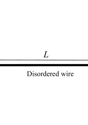
Figure 1: The setup. A disordered wire of length $L$ is in a good contact with two reservoirs, the entire system is in equilibrium. A small flux $I_{\rm in}$ of electrons with energy $E\gg T$ is sent to the left end of the wire through the left reservoir, and the part $I_{R}={\cal T}I_{\rm in}$ finally reaches the right reservoir.

Hot electrons, injected into the wire, weakly interact with the thermal bath, their energy is not conserved. However, as long as $E\gg T$, only the processes in which the energy is transferred from electron to the bath, not vice versa, are allowed. This is only true for not very long wires $L<L_{\rm Mott}(T)$, where $L_{\rm Mott}(T)\sim a(T_{0}/T)^{1/2}$ is the length of the typical Mott hop at given $T$. Under this condition the equilibration does not have chance to occur before the electrons escape from the wire. In this letter we also do not take into account correlation effects (like Coulomb gap) due to electron-electron interactions.

Obviously, only the localized states with the energies $\varepsilon_{i}$ in the interval between the Fermi energy and the initial energy $E$ of the injected electron are relevant for our problem. We enumerate them according to their energies: $0<\varepsilon_{1}<\varepsilon_{2}<\ldots<\varepsilon_{n}<E.$ These “quasiresonant” levels play an important role in the transport physics, as the electron, travelling through the chain with initial energy $E$, can make intermediate stops only at these sites. Indeed, all the sites with $\epsilon_{i}<0$ are occupied, while the sites with $\epsilon_{i}>E$ cannot be reached, as no energy can be absorbed. The spatial positions of quasiresonances are $\ell_{i}=Lx_{i}$, the independent random variables $x_{i}$ are homogeneously distributed in an interval $0<x_{i}<1$. The number $n$ of quasiresonances is itself a random variable, described by the poissonian distribution $p(n,N)=N^{n}\exp(-N)/n!$ , where $N=LEg$ is the average number of quasiresonances. Thus, each wire is characterized by “the configuration” ${\cal C}\equiv\{n,\{x_{1},\ldots x_{n}\}\}$ and the average of any ${\cal C}$-dependent quantity $A({\cal C})$ over the ensemble of wires is $\overline{A}=\sum_{n=0}^{\infty}p(n,N)\prod_{i=1}^{n}\int_{0}^{1}dx_{i}A({\cal C})$. In particular, the distribution function $F_{N}(s)=\overline{\delta(s-s({\cal C}))}$. In this letter we focus on the most interesting case $N\gg 1$, when the poissonian distribution is sharp and one can simply average over $x_{i}$ at fixed $n\approx N$.

How can an electron get from left reservoir to the right one? Besides the obvious possibility of the direct elastic tunnelling (Fig.2a), there are also numerous “inelastic staircases” (Fig.2b,c), in which an electrons makes intermediate stops at certain quasiresonant states, while the excess energy at each hop is transferred to the thermostat. Each staircase ${\cal S}$ is characterized by the choice of a subset of $K$ ($0\leq K\leq n$) quasiresonances, with $\varepsilon_{k_{1}}<\varepsilon_{k_{2}}<\cdots<\varepsilon_{k_{K}}$ and $x_{k_{1}}>x_{k_{2}}>\cdots>x_{k_{K}}$.

Each staircase contributes to the transmission:

$${\cal T}({\cal C})=\sum_{{\cal S}}{\cal T}({\cal S}|{\cal C})\propto e^{-\alpha s({\cal C})},\quad{\cal T}({\cal S}|{\cal C})\propto e^{-\alpha s({\cal S}|{\cal C})},$$ (4)

where the summation runs over all the staircases, possible for given configuration ${\cal C}$. Under the condition (2) the sum in (4) is dominated by only one – the optimal – staircase ${\cal S}_{\rm opt}({\cal C})$ that corresponds to minimal $s({\cal S}|{\cal C})$, so that $s({\cal C})\approx s[{\cal S}_{\rm opt}({\cal C})]=\min_{\cal S}s({\cal S}|{\cal C})$. In a typical situation the longest hop in the optimal staircase is the last one, then goes the last but one, etc. Therefore the value of $s({\cal S}|{\cal C})$ is controlled by few last hops in ${\cal S}$, while the multitude of short hops in the upper part of the staircase are of only secondary importance. The most natural assumption about the structure of the optimal staircase would be the scaling hypothesis: the distribution function ${\cal P}_{k}(\ell_{k})$ for random variables $\ell_{k}=x_{i_{k}}/x_{i_{k-1}}$ does not depend on $k$. Such a simple self-similar structure was, however, not observed in our numerical experiments: ${\cal P}_{k}$ manifestly depended on $k$.

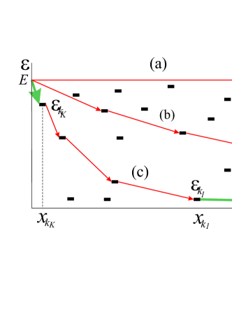
Figure 2: (color online) Possible scenarios for electron passing from the left to the right reservoir. “Natural hops” (occurring with the probability close to unity) are shown by thick green arrows, the non-natural hops (that happen with exponentially small probability) are shown by thin red arrows. (a): Direct elastic tunnelling; (b,c): Inelastic staircases with intermediate stops at quasiresonances.

The explicit expression for $s({\cal S}|{\cal C})$ can be found with the help of the stationary master equation for the quasiresonant levels populations $f_{i}$:

$$P_{L\to i}I_{\rm in}+\sum_{j>i}f_{j}P_{j\to i}-f_{i}P_{i\to{\rm out}}=0,$$ (5)

The first term in (5) is the incoming flux of particles from the left reservoir; the second term describes the particles, coming to the level $i$ from all other levels with higher energies (hence the condition $j>i$); finally, the third term takes into account all possible escapes from the $i$-th level: $P_{i\to{\rm out}}=P_{i\to L}+P_{i\to R}+\sum_{j<i}P_{i\to j}$. The system’s transmittance is

$${\cal T}\equiv I_{R}/I_{\rm in}=P_{L\to R}+\sum_{i}P_{i\to R}(f_{i}/I_{\rm in}).$$ (6)

The rate of transitions between $j\to i$ is $P_{j\to i}=P^{(0)}_{j\to i}(\varepsilon_{j}-\varepsilon_{i})e^{-\alpha|x_{i}-x_{j}|}$. Matrix elements of the electron-thermostat interaction, entering $P^{(0)}_{j\to i}$ are smooth power-law functions of the energy transfer $\varepsilon_{j}-\varepsilon_{i}$. It means, that if we are interested only in the exponential dependencies, we do not have to take these matrix elements into account. Thus, in the exponential approximation we can write

$$P_{i\to j}\propto\theta(i-j)e^{-\alpha|x_{i}-x_{j}|},\quad P_{i\to{\rm out}}\propto e^{-\alpha\chi_{i}},$$ (7)

$$\chi_{i}({\cal C})\equiv\min\left\{x_{i},1-x_{i},\min_{j<i}\{|x_{i}-x_{j}|\}\right\},$$ (8)

being the distance from the $i$-th quasiresonance to its “natural descendant” – a closest neighbor with lower energy, or to one of the two reservoirs. The solution of the system of equations (5) can be written in a recurrent form:

$$f_{i}=(P_{L\to i}/P_{i\to{\rm out}})I_{\rm in}+\sum_{j>i}f_{j}(P_{j\to i}/P_{i\to{\rm out}}),$$ (9)

which allows for finding $f_{i}$ provided all $f_{j}$ with $j>i$ are already found. According to the exponential approximation, justified by the large parameter (2), any sum, occurring in (6) or in (9), is dominated by a single term with the smallest negative exponent. As a result, the normalized probability for the electron to make a hop $i\to j$ is $p(i\to j)=P_{i\to j}/P_{i\to{\rm out}}=\exp\{-\alpha\Delta s(i\to j)\}$, where $\Delta s(i\to j)=|x_{i}-x_{j}|-\chi_{i}$. Then, having in mind that ${\cal T}({\cal S}|{\cal C})=\prod_{k=1}^{K+1}p(i_{k}\to i_{k-1})$, we arrive at

$$s({\cal S}|{\cal C})=\sum_{k=1}^{K+1}\Delta s(i_{k}\to i_{k-1}),$$ (10)

so that $\Delta s(i_{k}\to i_{k-1})$ has the meaning of the contribution of the $k$-th hop to the exponent $s$. In (10) $x_{0}=1$ and $x_{K+1}=0$ are the positions of the right and the left reservoirs, correspondingly; $\chi_{K+1}=0$. From (10) it immediately follows that $s({\cal S}|{\cal C})=1-\sum_{k=1}^{K+1}\chi_{i_{k}}$. In principle, our problem can be solved by means of enumeration of all staircases, possible for a given configuration, and choosing the optimal one. The direct solution of the master equations, however, leads to the same result.

Note, that $\Delta s(i_{k}\to i_{k-1})=0$ if the $i_{k-1}$-th quasiresonance is the natural descendant of the $i_{k}$-th one. The corresponding hops we will call “natural hops” in what follows. Clearly, to minimize $s$, it would be nice to have a staircase, where all the hops $i_{k}\to i_{k-1}$ (or at least as many of them, as possible) are natural. We will see, however, that such a “natural staircase” is possible to find only for some rare “fortunate configurations”.

Suppose that certain configuration ${\cal C}$ generates an optimal staircase, in which a sufficiently long subsequence of last $m$ hops ${k_{m}}\to{k_{m-1}}\to\cdots\to{k_{1}}\to R$ is “natural”, see Fig.3. It means that, if an electron somehow manages to get to the upper level ${k_{m}}$ in this subsequence, then it makes its descending way to the right reservoir through the rest of the staircase with a probability that is close to unity. Then, if this upper level is close enough to the left reservoir (namely, if $x_{k_{m}}<s$), then one can guarantee that $s({\cal C})<s$, no mater whether the preceding short hops in the staircase are natural or not.

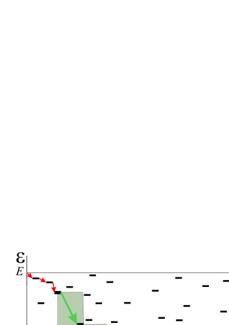
Figure 3: (color online) A “fortunate” configuration (with $m=5$). The last $m$ hops in an optimal staircase are “natural”. There are no quasiresonances in the shaded domain.

The necessary conditions for a given configuration ${\cal C}$ to be a fortunate one are as follows: The last jump (to $R$) should start from the lowest level (i.e., $k_{1}=1$), and this level should be localized in the right half of the wire: $x_{1}>1/2$. In general, the level $k_{p}$ in the optimal staircase should be the lowest one among all the quasiresonances with $0<x_{i}<x_{k_{p-1}}$; this level should be in the right half of the stretch: $x_{k_{p-1}}/2<x_{k_{p}}<x_{k_{p-1}}$. This should be true for all jumps with $p<m$, where $m$ is determined by the condition $x_{k_{m}}<s$.

The probability for all the $m$ last jumps in the optimal staircase to be natural is $2^{-m}$. However, $m$ is not determined solely by $s$: for fixed $s$ $m$ still fluctuates from configuration to configuration.

Let us introduce statistically independent random variables $\xi_{p}=2[x_{k_{p}}-x_{k_{p-1}}]/x_{k_{p-1}}$, homogeneously distributed in the interval $0<\xi_{p}<1$. Then $s=\prod_{p=1}^{m}(1+\xi_{p})/2$. The distribution $P_{m}(\phi)$ of the random variable $\phi=m\ln 2-\ln(1/s)=\sum_{p=0}^{m}\ln(1+\xi_{p})$ can be obtained with the help of the Fourier transformation:

$$P_{m}(\phi)=\int\frac{dq}{2\pi}e^{-iq\phi}\left[\frac{2^{iq+1}-1}{iq+1}\right]^{m},$$

$$F_{\infty}(s)\approx\sum_{m}2^{-m}\int d\phi P_{m}(\phi)\delta(s-\exp\{\phi-m\ln 2\})=$$

$$=\sum_{m}\frac{P_{m}(m\ln 2-\ln(1/s))}{s2^{m}}=\int\frac{dq}{2\pi s}\frac{(1+iq)e^{iq\ln(1/s)}}{2^{-(1+iq)}+iq}$$

$$\propto s^{-1}e^{-2\ln(1/s)}\approx bs.$$

where $b\sim 1$ is a universal constant. Although this asymptotics describes only a small fraction of the configurations, it turns out to be sufficient for finding the average transmission coefficient:

$$\overline{\mathcal{T}}\approx\int_{0}^{1}bs\exp\{-\alpha s\}ds=b\alpha^{-2}\propto L^{-2}.$$ (11)

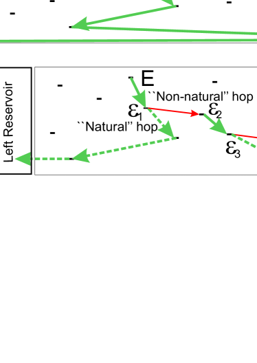
Figure 4: (color online) (a): The “natural path” consisting of hops to nearest neighbors with lower energy. The particle starts from the middle of the wire, so that in one half of the ensemble of samples the natural path leads the left reservoir, and it leads to the right one in the other half. (b): The particle is initially placed near the left reservoir, the natural path leads there in almost all samples. To get to the right reservoir, a particle has to make non-natural hops.

The hopping motion of hot particles, accompanied by the emission of energy, earlier was studied in the context of recombination of photo-excited electron-hole pairs Shklovskii . For that end it was sufficient to take into account only the natural hops since a particle was assumed to be created in the bulk, far from the ends of the sample, so that it could not escape to a nearby lead (see Fig.4a). Under these conditions the evolution of particle density profile, averaged over the ensemble of samples could be described by a peculiar diffusion, in which the distribution of hops lengths is rescaled by a fixed parameter $q>1$ after each hop. If one would extend the same approach to the setup where the particle is initially placed near one of the absorbing leads, then one easily finds for the probability to reach the opposite lead (and thus the average transmission coefficient) $\overline{\mathcal{T}}\propto L^{-\beta}$, where the exponent $\beta$ (as well as the parameter $q$) is universal. Note that this result is in agreement with (11). However, as we have already mentioned, $\overline{\mathcal{T}}$ is controlled by very rare anomalous samples with high transparency, while in a typical sample the natural path would lead to the nearby left lead (see Fig.4b). Therefore, to find the probability to reach the right lead in a typical sample one should take into account the non-natural hops, that were ignored in Shklovskii . The “diffusional approach” Shklovskii , being an adequate instrument for finding $\overline{\mathcal{T}}$, is useless for the determination of the distribution of ${\mathcal{T}}$.

The distribution $F_{N}(s)$ for general $s$ and $N$ can only be found numerically. We generated an ensemble of $\sim 10^{6}$ random configurations ${\cal C}$ and calculated corresponding $s({\cal C})$ with the help of the recurrent formula (9). The results of our Monte-Carlo simulations are summarized in Fig.5. The distribution functions $F_{N}(s)$ are wide: the dispersion of $s$ is of order of $\overline{s}$ for all $N$. For $N\gtrsim 300$ practically $F_{N}(s)\approx F_{\infty}(s)$, and $F_{\infty}(s)$ indeed shows a linear low-$s$ asymptotics with $b\approx 29$.

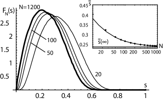
Figure 5: Distribution functions of the logarithm of transparency for different values of average number of quasiresonaces $N\equiv ELg$. For $N\gtrsim 200$ the curves practically merge and coincide with $F_{\infty}(s)$, shown by thick line. The $N$-dependence of the average logarithm of transmittance is shown on the inset, the solid line being the asymptotic expression (12).

The average value $\overline{s}(N)$ monotonically decreases with $N$, tending to a finite limit $\overline{s}(\infty)\approx 0.237$ at $N\to\infty$. The convergence is, however, extremely slow: for $N=1000$ the relative difference is still of order of $2\%$. The convergence can be improved dramatically if one introduces an asymptotic correction according to the empiric formula

$$\overline{s}(N)\approx 0.237+0.598\ln N/N,\qquad\mbox{for $N\gg 1$}.$$ (12)

The deviation of experimental $\overline{s}(N)$ from the asymptotics (12) is less than $2\%$ already for $N\sim 30$. The $N$-dependent corrections are controlled by many short hops in the beginning of the optimal staircase. The scaling hypothesis, mentioned above, would lead to $\overline{s}(N)-\overline{s}(\infty)\propto 1/N$, which is inconsistent with our numerical data. This is another argument against the scaling. A fit of our numerical data for the $N$-dependence of an average number $\overline{K}$ of hops in the optimal staircase gives

$$\overline{K}(N)\approx 0.39(\ln N)^{2}+2.4,\qquad\mbox{for $N\gg 1$}$$ (13)

which is perfectly consistent with the result (12) and, again, inconsistent with the scaling hypothesis, (the latter would give $\overline{K}(N)\propto\ln N$). The elucidation of the structure of the initial part of the optimal staircase and the origin of the empirical laws (12,13) still remains a challenge.

In conclusion, we have found the distribution function of the transmission coefficient for the inelastic penetration of a cold disordered wire by a hot electron. The applications of these results to specific physical effects will be presented in a long paper to follow.

We are indebted to M.E.Raikh for valuable comments.

References

- (1) P. W. Anderson, Phys. Rev. 109, 1492 (1958).
- (2) I. M. Lifshits, S. Gredescul, and L. A. Pastur, Introduction to the Theory of Disordered Systems (Wiley, New York, 1988).
- (3) V. L. Berezinskii, JETP, 38, 620 (1974).
- (4) P. W. Anderson, D. J. Thouless, E. Abrahams, and D. S. Fisher, Phys. Rev. B 22, 3519 (1980); P. W. Anderson, Phys. Rev. B 23, 4828 (1981).
- (5) B. I. Shklovskii and A. L. Efros, Electronic Properties of Doped Semiconductors (Springer-Verlag, Berlin, 1984).
- (6) J. Kurkijärvi, Phys. Rev. B 8, 922 (1973).
- (7) M. E. Raikh and I. M. Ruzin, JETP 68, 642 (1989).
- (8) T. Nattermann, T. Giamarchi, and P. Le Doussal, Phys. Rev. Lett. 91, 056603 (2003).
- (9) N. F. Mott, J. Non-Cryst. Solids, 1, 1 (1968); V. Ambegaokar, B. J. Halperin, and J. S. Langer, Phys. Rev. B 4, 2612 (1971).
- (10) M. M. Fogler and R. S. Kelley, Phys. Rev. Lett. 95, 166604 (2005).
- (11) A. S. Rodin and M. M. Fogler, Phys. Rev. B 80, 155435 (2009).
- (12) Nguyen Van Lien and B. I. Shklovskii, Sol. St. Comm., 38, 99 (1981).
- (13) B. I. Shklovskii, H. Fritzsche, and S. D. Baranovskii, Phys. Rev. Lett. 62, 2989 (1989).