Phase separation of binary condensates in harmonic and lattice potentials

Abstract

We propose a modified Gaussian ansatz to study binary condensates, trapped in harmonic and optical lattice potentials, both in miscible and immiscible domains. The ansatz is an apt one as it leads to the smooth transition from miscible to immiscible domains without any a priori assumptions. In optical lattice potentials, we analyze the squeezing of the density profiles due to the increase in the depth of the optical lattice potential. For this we develop a model with three potential wells, and define the relationship between the lattice depth and profile of the condensate.

I Introduction

After the successful experimental realization of two-species Bose-Einstein condensate (TBEC), consisting of different hyperfine spin states of ⁸⁷Rb Myatt ; Mertes ; Thalhammer , experimental as well as theoretical investigations in this field have come a long way. TBECs of different atomic species (⁴¹K and ⁸⁷Rb) Modugno and of different isotopes of same atomic species (⁸⁵Rb and ⁸⁷Rb) Papp have been experimentally observed. Phase separation, a typical feature of two component Bose-Einstein condensates, has been observed unambiguously Papp . A lot of static as well as dynamical properties of the TBECs have been analyzed in great detail in recent years. These include the ground state geometry Ho ; Chui1 ; Chui2 ; Trippenbach ; Timmermans ; Ao ; Barankov ; Schaeybroeck ; Gautam1 , modulational instability Kasamatsu1 ; Raju ; Ronen , Rayleigh-Taylor instability Gautam2 ,Sasaki , Kelvin-Helmholtz instability Takeuchi , etc..

The ground state geometry of the TBEC has been studied, semi-analytically, using Thomas-Fermi (TF) approximation Ho ; Chui1 ; Chui2 ; Trippenbach . These works did not take into account the contribution of the interface energy explicitly. The interface energy was taken into account in some other works Timmermans ; Ao ; Barankov ; however, the interface energy correction incorporated in these works was not good enough to reproduce the experimentally observed ground state structures with planar interface Papp . A more accurate analytic approximation to account for interface energy was suggested by Schaeybroeck et al. Schaeybroeck , and a recent work Gautam1 conclusively proved that using this analytic approximation for interface energy in TF regime, planar and cylindrical geometries emerge as the ground state structures in cigar and pan-cake shaped trap potentials. The common salient feature of all these works is the use of TF approximation, which is a good approximation for large number of atoms of each species. In fact if $N,~{}a$, and $a_{\rm osc}$ are respectively, number of atoms of the component species, s-wave scattering length, and oscillator length, TF approximation is valid provided $Na/a_{\rm osc}\gg 1$. Obviously, this condition is not satisfied for attractive condensates. For small number of atoms as well, say of the order of a few hundreds, and for very weakly interacting condensates ($a/a_{\rm osc}\ll 1$), the contribution of the kinetic energy to the total energy is significant and can not be merely treated as a correction to total energy as is done in TF based approaches. For such TBECs, TF approximation is not a good approximation, and hence can not be relied upon to determine the ground state structure of the TBEC. In present work, we analyze the ground sate properties of the TBECs using suitable ansatz in both miscible and immiscible regimes. The Gaussian nature of the ansatz makes our approach better equipped to study the stationary state properties of the of very weakly interacting ($Na/a_{\rm osc}\sim 1$) TBECs and also those with attractive interactions. With the advent of Feshbach resonances Chin , it is experimentally possible to tune scattering lengths to reach the very weakly interacting regime or even non-interacting regime Weber ; Kraemer ; Roati . Magnetic Feshbach resonances can tune only one scattering length independently, whereas optical Feshbach resonances Fedichev open up the possibility of tuning different scattering length in a multicomponent system independently. With the experimental observation of optical Feshbach resonances in ¹⁷²YbEnomoto and ¹⁷⁴Yb Yamazaki , experimental realization of weakly interacting regime in binary condensates appears a distinct possibility. The present approach, thus, supplements TF based semi-analytic schemes to determine the ground state geometries of the TBECs.

Keeping a pace with the studies on TBECs, has been the realization of various condensed matter phenomena like ac Josephson effect, Bloch oscillations, Landau-Zener tunneling, etc. in single species Bose-Einstein condensates (BECs) trapped in optical lattices Anderson ; Burger ; Cataliotti ; Morsch . Superfluid-Mott insulator transition has been also observed with BECs in optical lattice potentials Greiner . In mean field approximation, we also study the ground sate geometry of TBECs trapped in optical lattice potentials using discrete nonlinear Schrödinger equation (DNLSE) Trombettoni . We also compare our semi-analytic results with the numerical solution of coupled Gross-Pitaevskii equations and find a very good agreement especially in very weakly interacting regime.

II TBECs in axisymmetric traps

In this section, we provide a general variational scheme to study the stationary state geometry of TBECs in axisymmetric trap potentials

$$V_{i}(r,z)=\frac{m_{i}\omega^{2}}{2}(r^{2}+\alpha_{i}^{2}z^{2}),$$ (1)

where $i=1,2$ is the species index, $\omega$ is the radial trap frequency for two components, and $\alpha_{i}$ are the anisotropy parameters. For simplicity of analysis, we consider trap potentials for the component species are identical $\alpha_{1}=\alpha_{2}=\alpha$ and $m_{1}=m_{2}=m$. The ground state of the TBEC is described by a set of coupled GP equations

$$\left[\frac{-\hbar^{2}}{2m}\nabla^{2}+V_{i}(r,z)+\sum_{j=1}^{2}U_{ij}|\Psi_{j}|^{2}\right]\Psi_{i}=\mu_{i}\Psi_{i},$$ (2)

in mean field approximation, where $i=1,2$ is the species index. Here $U_{ii}=4\pi\hbar^{2}a_{ii}/m_{i}$, where $m_{i}$ is the mass and $a_{ii}$ is the $s$-wave scattering length, is the intra-species interaction, $U_{ij}=2\pi\hbar^{2}a_{ij}/m_{ij}$, where $m_{ij}=m_{i}m_{j}/(m_{i}+m_{j})$ is the reduced mass and $a_{ij}$ is the inter-species scattering length, is the inter-species interaction, and $\mu_{i}$ is the chemical potential of the $i$th species. The energy of the TBEC is

$$E = \int_{-\infty}^{\infty}\left[\sum_{i=1}^{2}\left(\frac{\hbar^{2}}{2m}|\nabla\Psi_{i}|^{2}+V_{i}(r,z)\Psi_{i}^{2}\right.\right.$$ (3)

$$\left.\left.+\frac{U_{ii}}{2}|\Psi_{i}|^{4}\right)+U_{12}|\Psi_{1}|^{2}|\Psi_{2}|^{2}\right]d{\bf r}.$$

To rewrite the energy in suitable units, define the oscillator length of the trapping potential

$$a_{\rm osc}=\sqrt{\frac{\hbar}{m\omega}},$$ (4)

and consider $\hbar\omega$ as the unit of energy. We then divide the Eq.(3) by $\hbar\omega$ and apply the transformations

$$\tilde{r}=\frac{r}{a_{\rm osc}},~{}\tilde{z}=\frac{z}{a_{\rm osc}},~{}\tilde{t}=t\omega,\text{and}~{}\tilde{E}=\frac{E}{\hbar\omega}.$$ (5)

The transformed order parameter

$$\phi_{i}(\tilde{r},\tilde{z})=\sqrt{\frac{a_{\rm osc}^{3}}{N_{i}}}\Psi_{i}(r,z),$$ (6)

and energy of the TBEC in scaled units is

$$\tilde{E} = \int d\tilde{{\bf r}}\left\{\sum_{i=1}^{2}N_{i}\left[\frac{1}{2}|\nabla\phi_{i}|^{2}+V_{i}(\tilde{r},\tilde{z})|\phi_{i}|^{2}+\right.\right.$$ (7)

$$\left.\left.N_{i}\frac{\tilde{U}_{ii}}{2}|\phi_{i}|^{4}\right]+N_{1}N_{2}\tilde{U}_{12}|\phi_{1}|^{2}|\phi_{2}|^{2}\right\},$$

where $\tilde{U}_{ii}=4\pi a_{ii}/a_{\text{osc}}$ and $\tilde{U}_{12}=4\pi a_{12}/a_{\text{osc}}$ in the scaled units. For simplicity of notations, from here on we represent the transformed quantities without tilde. We obtain the coupled 2D GP equations,

$$\left[-\frac{1}{2}\frac{\partial^{2}}{\partial r^{2}}-\frac{1}{2r}\frac{\partial}{\partial r}+V_{i}(r,z)+\sum_{j=1}^{2}G_{ij}|\phi_{j}|^{2}\right]\phi_{i}=\mu_{i}\phi_{i},$$ (8)

when the energy functional ${\cal E}=E-\sum_{i}\mu_{i}N_{i}$ is variationally minimized with $\phi_{i}^{\star}$ as parameters of variation, here $G_{ii}=N_{i}\tilde{U}_{ii}$ and $G_{ij}=N_{j}\tilde{U}_{ij}$. The equations are then solved numerically. Another approach ideal for semi-analytic treatment is to adopt a predefined form of $\phi$ with few variational parameters and minimize $E$. This is outlined for the 2D and 1D in the next subsections.

II.1 Variational ansatz

As mentioned earlier, the ground state of TBEC can be either be miscible or immiscible depending on the interaction parameters. An ansatz which describes the ground state of the TBEC well, both in the miscible and immiscible domain, when $a_{ii},a_{ij}>0$ and $a_{22}>a_{11}$ is

$$\Psi_{1}(r,z) = ae^{-(r^{2}+\alpha^{2}z^{2})/(2b^{2})},$$

$$\Psi_{2}(r,z) = \left[f+c(r^{2}+\alpha^{2}z^{2})\right]e^{-(r^{2}+\alpha^{2}z^{2})/(2d^{2})},$$ (9)

with $a,~{}b,~{}f,~{}c$, and $d$ as the variational parameters. In the phase separated or immiscible domain, this ansatz is apt for the ellipsoidal interface geometry where the density distribution follows the equipotential surfaces of the trapping potentials. It is applicable, in particular, to weakly interacting TBECs, and this is precisely the underlying assumption for choosing the present ansatz. This ansatz is not suitable for analysis of planar and cylindrical geometries where density distributions do not follow equipotential surfaces. A similar ansatz, perhaps more general, is used in ref. Adhikari to examine symbiotic gap and semi gap solitons in TBECs trapped in optical lattice potentials. The parameter $c$ accounts for the flattening of the density profile of the second species as the intra-species non-linearity is increased. Moreover, for symmetric ground state geometries, $c$ is a parameter related to the overlap of two component wave functions. For an ideal case when all the non-linearities are small and equal, $c$ is $\approx 0$, and hence the two species of the TBEC completely overlap.

If $N_{1}$ and $N_{2}$ are the number of particles of the two species, then from Eq.(6) in scaled units

$$\int_{-\infty}^{\infty}d{\bf r}|\phi_{i}(r,z)|^{2}=1.$$ (10)

Since the number of atoms of each species is fixed, the normalization conditions are equivalent to two constraint equations and reduce the number of variational parameters by two. After evaluating the integrals, the two constraint equations are

$$b = \frac{(-1)^{2/3}\alpha^{1/3}}{a^{2/3}\sqrt{\pi}},$$

$$c = \frac{2\sqrt{3}}{15d^{7}}\left(\frac{\sqrt{5d^{7}\pi^{3/2}\alpha-2d^{10}f^{2}\pi^{3}}}{\pi^{3/2}}-\sqrt{3}d^{5}f\right).$$ (11)

From Eqs.(7-10), the energy of the first species is

$$E_{1}=\frac{a^{2}bN_{1}\pi^{3/2}}{8\alpha}\left(\sqrt{2}a^{2}b^{2}G_{11}+4+6b^{4}+2\alpha^{2}\right),$$ (12)

similarly, for the second species

$$E_{2} = \frac{dN_{2}\pi^{3/2}}{2048\alpha}\left\{128\left[4f^{2}\left(2+3d^{4}+\alpha^{2}\right)+4cd^{2}f(2\right.\right.$$ (13)

$$\left.+15d^{4}+\alpha^{2})+c^{2}d^{4}(22+105d^{4}+11\alpha^{2})\right]$$

$$+\sqrt{2}d^{2}G_{22}(945c^{4}d^{8}+1680c^{3}d^{6}f+1440c^{2}d^{4}f^{2}$$

$$\left.+768cd^{2}f^{3}+256f^{4})\right\},$$

and the energy from the inter species interaction is

$$E_{12} = \frac{2N_{1}G_{12}b^{2}d^{3}\pi^{3/2}}{2048\alpha(b^{2}+d^{2})^{7/2}}\left[15b^{4}c^{2}d^{4}+12b^{2}cd^{2}f(b^{2}\right.$$ (14)

$$\left.+d^{2})+4f^{2}(b^{2}+d^{2})^{2}\right].$$

We can then define the energy per boson as

$$\epsilon=\frac{E_{1}+E_{2}+E_{12}}{N_{1}+N_{2}}.$$ (15)

This can now be minimized numerically to determine variational parameters and hence the ground state wave functions. The results of minimization with the parameters satisfying $N_{i}a_{ij}/a_{osc}\sim 1$ are shown in Fig.1 along with the corresponding numerical results.

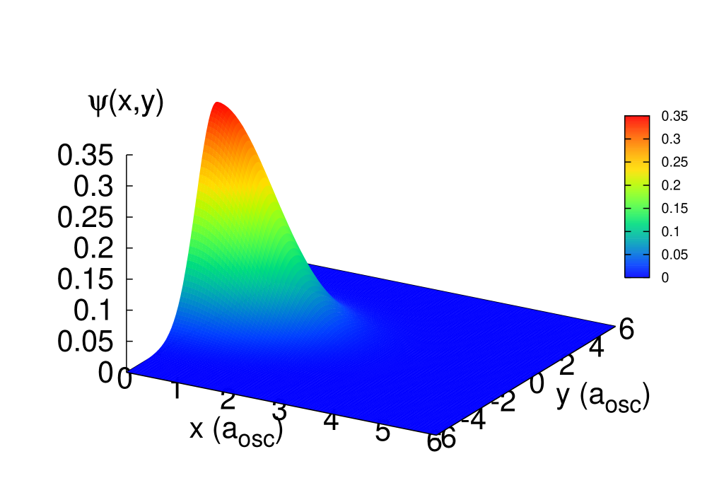
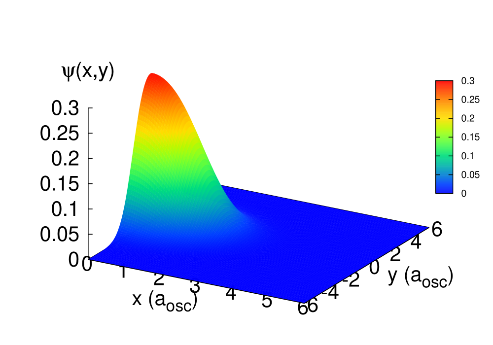
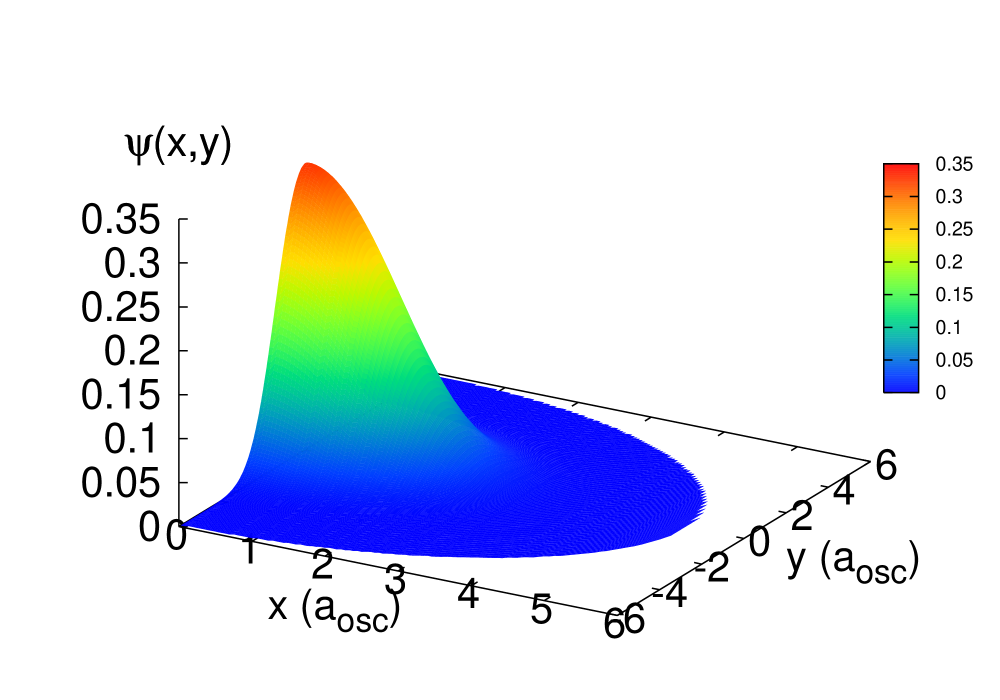
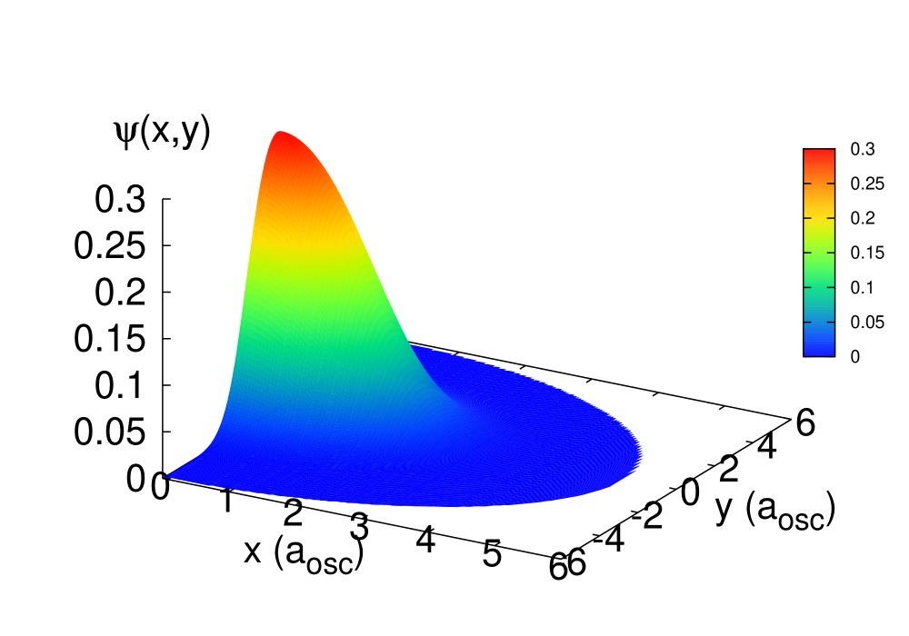
Figure 1: The semi-analytic and numerical profiles for a binary condensate with $N_{1}=N_{2}=10,000$, $\alpha=0.8$, $a_{osc}=9.566\times 10^{-7}m$, $a_{11}=0.5a_{0}$, $a_{22}=1.0a_{0}$, and $a_{12}=0.8a_{0}$. Starting from left, the upper panel shows the semi-analytic profiles for the first and the second component, exactly below them in lower panel are wave function profiles obtained by numerically solving Eq.(8).

It should be noted that the scenario of all the non-linearities to be equal ($N_{1}=N_{2}$ and $a_{ii}=a_{ij}$) is not equivalent to single component condensate with $a_{ii}=a_{ij}=a_{s}$ as the $s$-wave scattering length and total number of atoms equal to $N_{1}+N_{2}$. This is due to fact that we are still treating the two components as two different species having order parameters $\phi_{1}(r,z)$ and $\phi_{2}(r,z)$. It means that experimentally, even if for two different hyperfine states of an isotope above condition is satisfied, the system will be still a binary system having a pair of ground state wave functions $\phi_{1}(r,z)$ and $\phi_{2}(r,z)$ instead of single ground state wave function for single component BEC. Quantum mechanically, it means that for the system to behave as a single species BEC, the two components needs to be indistinguishable with the same wave function $\phi(r,z)$.

II.2 Quasi-1D condensates

When the radial trapping frequency is much larger than axial trapping frequency ($\alpha\ll 1$), and the TBEC is in the weakly interacting regime $a_{i}N_{i}|\psi(z)|^{2}\ll 1$, the order parameter can be factorized into radial and axial parts

$$\phi_{i}(r,z)=\xi_{i}(r)\psi_{i}(z),$$ (16)

where $\xi_{i}(r)$ is the normalized ground state of radial trapping potential $V_{i}^{\rm rad}=r^{2}/2$. From Eq.(7), after integrating out the radial order parameter, the energy of the quasi-1D system is

$$E = \int_{-\infty}^{\infty}\left[\sum_{i=1}^{2}N_{i}\left(\frac{1}{2}|\nabla_{z}\psi_{i}|^{2}+V_{i}^{a}(z)|\psi_{i}|^{2}+\right.\right.$$ (17)

$$\left.\left.N_{i}\frac{u_{ii}}{2}|\psi_{i}|^{4}\right)+N_{1}N_{2}u_{12}|\psi_{1}|^{2}|\psi_{2}|^{2}\right]dz,$$

where $u_{ii}=2a_{ii}$, $u_{12}=2a_{12}$, and $V_{i}^{a}(z)=\alpha^{2}z^{2}/2+1$. We analyze the ground state of the of repulsive TBEC $a_{ii},a_{ij}>0$ trapped in quasi-1D traps in both miscible $a_{12}\leq\sqrt{a_{1}a_{2}}$ and immiscible $a_{12}>\sqrt{a_{11}a_{22}}$ domains. Without loss of generality we assume $a_{22}>a_{11}$ and hence, the first species, on account of lower repulsive mean field energy, has larger density at the center when $N_{1}\approx N_{2}$. We consider

$$\psi_{1}(z) = ae^{-(z-\gamma)^{2}/(2b^{2})},$$

$$\psi_{2}(z) = (f+cz^{2})e^{-(z+\delta)^{2}/(2d^{2})},$$ (18)

as our ansatz for the two order parameters with $a,~{}\gamma,~{}b,~{}f,~{}c,~{}\delta$, and $d$ as variational parameters. Here $\gamma$ and $\delta$ represent the location of the order parameter maxima and center of mass motion. This is an apt ansatz as it describes the smooth transition between miscible and immiscible phases of the TBEC in a very natural way.

In the miscible domain, the parameter $c$ is a measure of flatness of the $\psi_{2}$ profile which arises from the larger intra-species repulsion energy. However, in the immiscible domain, it is the degree of separation between the two species due to the higher inter-species repulsion energy. The order parameters, like in previous subsection, satisfy the normalization conditions

$$\int_{-\infty}^{\infty}dz|\psi_{i}(z)|^{2}=1,$$ (19)

where $\psi_{i}(z)=\sqrt{a_{\rm osc}/N_{i}}\Psi(za_{\rm osc})$, and hence the number of independent variational parameters is reduced to five. From Eq.(17), Eq.(18), and Eq.(19), we obtain the expression for energy as a function of five independent parameters. It is a complicated eighth degree polynomial (given in appendix) and can not be solved analytically. However, one can treat it as a nonlinear optimization problem and use numerical schemes like Nelder-Meade to find a solution Press . Like in Eq.(8), the coupled 1D GP equations

$$\left[-\frac{1}{2}\frac{\partial^{2}}{\partial z^{2}}+V_{i}^{a}(z)+\sum_{j=1}^{2}g_{ij}|\psi_{j}|^{2}\right]\psi_{i}=\mu_{i}\psi_{i},$$ (20)

are obtained when ${\cal E}=E-\mu_{i}N_{i}$ is variationally extremized with $\psi_{i}^{\star}$ as the variational parameters, where $g_{ii}=N_{i}u_{ii}$ and $g_{ij}=N_{j}u_{ij}$.

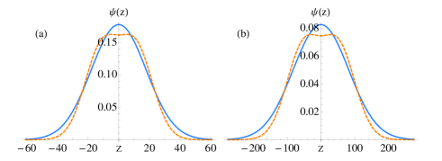
Figure 2: Order parameters $\psi_{i}$ of the two components from the variational calculations with equal intra-species scattering length of $51a_{0}$ but no inter-species interaction ($a_{ij}=0$). Solid (blue) and dashed (orange) correspond to the first and second species, respectively. The figure on the left hand side is for $N_{1}=N_{2}=1000$, while that on the right hand side is for $N_{1}=N_{2}=100,000$. The trapping potential parameters are $\alpha=0.02$ and $a_{\rm osc}=9.566\times 10^{-7}m$. For (a) $N_{i}a_{ii}/a_{osc}=2.821$ and for (b) $N_{i}a_{ii}/a_{osc}=282.137$.

II.2.1 Miscible domain with $a_{12}=0$

As mentioned earlier, the inequality $a_{12}<\sqrt{a_{11}a_{22}}$ defines the miscible domain. In this parameter range, the two order parameters overlap and in the limiting case of $a_{12}=0$, the two maxima coincide if $a_{11}=a_{22}$. Furthermore, in the non-interacting limit $a_{ij}\rightarrow 0$, the profiles of the two order parameters are identical for the same number of atoms ($N_{1}=N_{2}$). For the special case of identical intra-species scattering lengths ($a_{11}=a_{22}$), finite inter-species interaction ($a_{12}\neq 0$), and identical number of atoms ($N_{1}=N_{2}$), an appropriate ansatz is Navarro

$$\psi_{1}(z) = Ae^{-(z-B)^{2}/(2W^{2})}e^{i(C+Dz+Ez^{2})},$$

$$\psi_{2}(z) = Ae^{-(z-B)^{2}/(2W^{2})}e^{i(C-Dz+Ez^{2})},$$ (21)

originally introduced to describe dynamics of coupled solitons in nonlinear optical fibers Muraki . Here, the parameters $A$, $B$, $C$, $D$, $E$, and $W$ are assumed to be time dependent and represent the amplitude, position, phase, wave number, chirp, and width of the Gaussian ansatz, respectively. In our ansatz too, a more symmetric choice of the order parameters

$$\psi_{i}(z)=(f_{i}+c_{i}z^{2})e^{-(z-\gamma_{i})^{2}/(2b_{i}^{2})},$$ (22)

can represent the special case mentioned here. The expression of the energy is then much more complicated, and the situation considered being too restrictive, we do not consider this for further analysis and discussion. However, to examine the ground state geometry for a varied range of parameters, interaction strengths, and number of atoms, the ansatz in Eq.(18) is an ideal choice.

With our ansatz, when $a_{11}=a_{22}\neq 0$, $a_{12}=0$, and $N_{1}=N_{2}$, the $cz^{2}$ dependence in $\psi_{2}$ accounts for the self interaction. For this reason, the profile of $\psi_{2}$ is broader and more accurate, whereas $\psi_{1}$ is a Gaussian and does not reflect the effect of the self interaction in the profile in an equally precise manner as $\psi_{2}$. To examine the density profiles as function of the nonlinearity, arising from the mean field interaction, consider TBEC with $N_{i}=100,1000,$ and $10000$. As a specific case take $a_{11}=a_{22}=51$, which corresponds to ⁸⁵Rb Cornish , however, to begin with set $a_{12}=0$. The later is experimentally not realizable in ⁸⁵Rb, but it is a good reference for a comparative study on the role of inter-species interactions. The order parameters for the different $N_{i}$ with the chosen parameters are as shown in Fig.2. As mentioned earlier, the $\psi_{2}$ profiles are flatter and closer to the numerical values. Ideally, the two profiles should be identical as there is no inter-species interaction ($a_{12}=0$). So the difference between the profiles of the two order parameters is an indication of the error due to the Gaussian ansatz of $\psi_{1}$. From the figures, the deviation grows as $N_{i}$ is increased, which is expected as the mean field contribution to $E$ is quadratic in $N$. In the weakly interacting domain $c<1$ and contributions to $E$ from higher order terms of $c$ are negligible. Retaining only the linear terms, the energy correction arising from the mean field is

$$\Delta E \approx \frac{cfN_{2}\sqrt{\pi}}{4}\left[\frac{2\delta^{2}-d^{2}}{d}+d\alpha^{2}(3d^{4}+12d^{2}\delta^{2}\right.$$ (23)

$$+4\delta^{4})+\sqrt{2}df^{2}g_{22}(d^{2}+4\delta^{2})\bigg{]}.$$

For identical trapping potentials $V_{1}=V_{2}$, the order parameters $\psi_{i}$ are centered at the origin ( $z=0$) and hence $\delta\approx 0$. The energy correction then simplifies to

$$\Delta E\approx\frac{cdfN_{2}\sqrt{\pi}}{4}(3\alpha^{2}d^{4}+\sqrt{2}d^{2}f^{2}g_{22}-1).$$ (24)

The three terms are the leading order corrections from the trapping potential, mean field, and kinetic energy, respectively. Considering that in quasi 1D case $\alpha\ll 1$, the correction arising from $c$ is a competition between the mean field and kinetic energy contributions; at lower values of $g_{22}$, the kinetic energy correction dominates and $\Delta E$ is negative. As mentioned earlier for identical intra-species scattering lengths ($a_{11}=a_{22}$), Eq.(21) is more appropriate ansatz and for parameters of Fig.2(b) the ground state geometry of the TBEC is shown in Fig.3

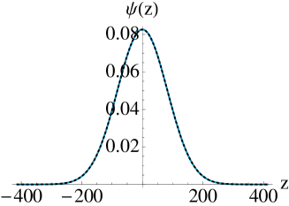
Figure 3: Order parameters $\psi_{i}$ of the two components from the variational calculations using Eq.(21) with equal intra-species scattering length of $51a_{0}$ but no inter-species interaction ($a_{ij}=0$). Solid (turquoise) and dotted (black) correspond to the first and second species, respectively. The number of atoms and trapping potential parameters are same as those in Fig.2(b).

II.2.2 Miscible domain with $a_{12}>0$

Finite inter-species interaction ($a_{12}\neq 0$) modifies the density profiles of the two species in a dramatic way. As $a_{12}$ is increased, the species with the higher repulsion energy, second in the present case, is repelled from the center of trap. This is noticeable in the profiles of TBEC shown in Fig.(4). The lower density of the second species, around the center of the trap decreases inter-species density product $|\psi_{1}|^{2}|\psi_{2}|^{2}$ and minimizes the total energy. However, this must be in proportion with the higher energy from trapping potential due to broader density profile. For identical trapping potentials ($V_{1}=V_{2}$), the profiles of the two species are centered at the origin ($\gamma=\delta=0$) and symmetric. From Eq.(70) in appendix, the inter-species interaction energy is

$$E_{12}^{\rm sym} = \frac{\sqrt{\pi}a^{2}bdN_{1}g_{12}}{4(b^{2}+d^{2})^{9/2}}\bigg{[}4d^{8}f^{2}+4b^{2}d^{6}(4f^{2}+cd^{2}f)$$ (25)

$$+b^{8}(4f^{2}+4cd^{2}f+3c^{2}d^{4})+2b^{6}d^{2}(8f^{2}+3c^{2}d^{4}$$

$$+6cd^{2}f)+b^{4}d^{4}(24f^{2}+3c^{2}d^{4}+12cd^{2}f)\bigg{]}.$$

Geometrically, with higher $a_{12}$ the shape of $\psi_{2}$ near potential minima undergoes a smooth transition from Gaussian to flat Fig. 4(a-b) and then, to parabola with a local minima at the center of the trap Fig. 4(c-d).

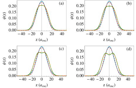
Figure 4: Ground state wave functions for the two components of the TBEC with $N_{1}=N_{2}=10000$, $g_{11}=0.553$, $g_{22}=2g_{11}$, $\alpha=0.02$ and $a_{osc}=9.566\times 10^{-7}m$. Starting from left, the values of $g_{12}$ are $0.1g_{22},0.3g_{22}$ in upper panel; and $0.5g_{22}$ and $0.7g_{22}$ in lower panel, respectively. The criterion, $N_{j}a_{ij}/a_{osc}=g_{ij}/2\sim 1$, for the applicability of the variational ansatz is satisfied for each case. Turquoise (reddish-brown) and dark-green(orange) curves correspond to first and second component, respectively; solid curves are semi-analytic results, while dashed ones are the numerical solutions of Eq.(20).

When $\psi_{2}$ is flat around the center, to a very good approximation $\psi_{2}^{\prime}(z)=\psi_{2}^{\prime\prime}(z)=0$ for $z<1$. With our ansatz $\psi_{2}^{\prime\prime}(0)$ is not zero when $a_{12}>0$, so there are deviations from the actual solutions. Deviations are negligible when $0<a_{12}\ll 1$, however, these grow and become quite prominent when $\psi_{2}$ is constant around the center of the trap.

At the center of the trap $\psi_{1}$ has the global maximum and $\psi_{1}^{\prime}(0)=0$. Close to the center the order parameter

$$\psi_{1}(z)\approx\psi_{1}(0)+\frac{z^{2}}{2}\psi_{1}^{\prime\prime}(0),$$ (26)

when $z<1$. Gaussian ansatz of $\psi_{1}$ defined in Eq.(18) then gives

$$\psi_{1}(z)\approx a-\frac{z^{2}}{2}\frac{a}{b^{2}}.$$ (27)

For the parameter domain where $\psi_{2}$ is constant close to the center for $z<1$, we can write

$$\psi_{2}(z)\approx\psi_{2}(0).$$ (28)

After substituting these expressions of $\psi_{i}$ in Eq.(20), the chemical potential of the two species obtained from the zeroth order equations are

$$\mu_{1} = \frac{1}{2b^{2}}+g_{11}a^{2}+g_{12}\psi_{2}(0)+1,$$

$$\mu_{2} = g_{22}\psi_{2}^{2}(0)+g_{21}a^{2}+1.$$ (29)

Since $\psi_{i}^{\prime}(0)=0$, the first order terms are zero, and hence second order equation of $\psi_{1}$ is

$$\left[\frac{\alpha^{2}}{2}+\frac{3g_{11}}{2}\psi_{1}(0)\psi_{1}^{\prime\prime}(0)\right]\psi_{1}(0)+\frac{g_{12}}{2}\psi_{2}(0)\psi_{1}^{\prime\prime}(0)=\frac{\mu_{1}}{2}\psi_{1}^{\prime\prime}(0).$$ (30)

Further simplifications provide the condition

$$g_{11}=\frac{1}{2a^{2}}\left(\frac{1}{2b^{2}}+\alpha^{2}b^{2}+1\right)$$ (31)

on the intra-species interaction of the first species. Similarly, the second order equation of $\psi_{2}$ is

$$\left[\frac{\alpha^{2}}{2}+g_{21}\psi_{1}(0)\psi_{1}^{\prime\prime}(0)\right]\psi_{2}(0)=0.$$ (32)

This defines the inter-species interaction as

$$g_{21}=\frac{\alpha^{2}b^{2}}{2a^{2}},$$ (33)

to obtain a constant profile of $\psi_{2}$ around center of the trap. In other words when this condition holds true, the repulsive inter-species interaction balances the effect of confining potential. And the net outcome is an effective potential around the center which is constant. The $\psi_{2}$ profile acquires a local minimum at the center when $g_{21}>\alpha^{2}b^{2}/(2a^{2})$, our ansatz is then the appropriate form of $\psi_{2}$.

II.2.3 Immiscible domain: symmetric profile

Phase separation occurs when the TBEC is immiscible. The density profiles of the two species are then spatially separated. Condition for immiscibility is $a_{12}>\sqrt{a_{11}a_{22}}$ when the TBEC is confined within a square well potential Ao . In which case, the trapping potential is flat and except for the surface effects, limited to within healing length $\xi=\sqrt{\hbar^{2}/(2m\mu)}$ from the boundary, there are no trapping potential induced density variations. The TBEC is then homogeneous in the miscible domain and phase separated in the immiscible domain, where the interface acquires a geometry which minimizes the surface energy. Here, the density distributions in the bulk is entirely dependent on the strength of interactions. And transition into phase separated domain is well defined.

With harmonic trapping potentials the densities, to begin with, are not homogeneous in the miscible phase. Even when $a_{12}<\sqrt{a_{11}a_{22}}$, miscible domain discussed previously, there is a separation between the two maxima of the densities. When $N_{1}\approx N_{2}$ and $a_{11}\approx a_{22}$, the density profiles are symmetric about the center ($\delta=\gamma=0$) and total energy of the TBEC is

$$E = \frac{\sqrt{\pi}}{4}\left[\frac{a^{2}N_{1}}{b}+a^{2}b^{3}\alpha^{2}N_{1}+\frac{N_{2}}{4d}(4f^{2}-4cd^{2}f\right.$$ (34)

$$+7c^{2}d^{4})+\frac{d\alpha^{2}N_{2}}{4}(4d^{2}f^{2}+12cd^{4}f+15c^{2}d^{6})$$

$$+\sqrt{2}a^{4}bN_{1}g_{11}+\sqrt{2}d\left(f^{4}+cd^{2}f^{3}+\frac{9}{8}c^{2}d^{4}f^{2}\right.$$

$$\left.\left.+\frac{15}{16}c^{3}d^{6}f+\frac{105}{256}c^{4}d^{8}\right)N_{2}g_{22}\right]+E_{12}^{\rm sym},$$

where $E_{12}^{\rm sym}$ is the inter-species interaction energy defined in Eq.(25). For the TBEC in square well described earlier, the criterion for phase separation Ao is the emergence of a dip in the total density $\rho_{1}(z)+\rho_{2}(z)=|\psi_{1}(z)|^{2}+|\psi_{2}(z)|^{2}$ at the interface. Such a criterion does not apply for TBEC in harmonic potentials. Instead we define phase separation as the state when the maxima of the densities are well separated. To quantify, define $z_{\rm e}$ as the point where the densities of the two species are equal, which implies

$$ae^{-z_{\rm e}^{2}/(2b^{2})}=(f+cz_{\rm e}^{2})e^{-z_{\rm e}^{2}/(2d^{2})}.$$ (35)

For large $a_{12}$, the order parameter $\psi_{2}(z)$ is bimodal. The two maxima are solutions of $\psi_{2}^{\prime}(z)=0$ and located at

$$z_{\rm m}=\pm\left(\frac{4cd^{2}-f}{c}\right)^{1/2}.$$ (36)

The maxima of $\psi_{2}$ are well separated from $\psi_{1}$ when $z_{\rm m}>z_{\rm e}$. We define this as the criterion for phase separation of TBEC in harmonic potentials. This definition of phase separation is an appropriate one in very weakly interacting TBECs $Na/a_{osc}\approx 1$, but not so in TF regime $Na/a_{osc}\gg 1$, where $f=0$ is a better criterion to define phase separation.

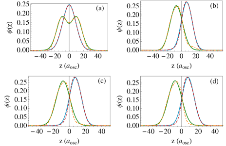
Figure 5: Ground state wave functions for the two components of the TBEC with $N_{1}=N_{2}=10000$, $g_{11}=0.553$, $g_{22}=2g_{11}$, $\alpha=0.02$ and $a_{osc}=9.566\times 10^{-7}m$. Starting from left, the values of $g_{12}$ are $0.9g_{22},1.2g_{22}$ in upper panel; and $1.4g_{22}$ and $1.6g_{22}$ in lower panel,respectively. The criterion, $N_{j}a_{ij}/a_{osc}=g_{ij}/2\sim 1$, for the applicability of the variational ansatz is satisfied for each case.Turquoise (reddish-brown) and dark-green (orange) curves correspond to first and second component, respectively; solid curves are semi-analytic results, while dashed ones are the numerical solutions of Eq.(20).

II.2.4 Imiscible domain: non-symmetric profile

In imiscible domain, if one or both the intra-species non-linearities $g_{ii}$ are sufficiently small, the stationary state geometry with symmetric $\psi_{i}$ can have higher energy than the asymmetric stationary state with the two components lying side by side. There are two reasons for the emergence of asymmetric ground state geometries. First, this geometry has only one interface region, whereas the corresponding symmetric profile has two; as a result the interface energy is lower. And second, smaller kinetic energy as $\psi_{i}^{\prime}(z)$ is prominent at the interface and edges of the condensates.

With our ansatz, for the asymmetric profile $c\sim 0$, but $\delta$ and $\gamma$ are nonzero. The total energy of the TBEC is then

$$E = \frac{\sqrt{\pi}}{4}\bigg{[}\frac{a^{2}N_{1}}{b}+\frac{f^{2}N_{2}}{d}+a^{2}b\alpha^{2}N_{1}(b^{2}+2\gamma^{2})$$ (37)

$$+df^{2}\alpha^{2}N_{2}(d^{2}+2\delta^{2})+\sqrt{2}a^{4}bN_{1}g_{11}+\sqrt{2}df^{4}N_{2}g_{22}$$

$$+\frac{4a^{2}bde^{-(\gamma+\delta)^{2}/(b^{2}+d^{2})}}{(b^{2}+d^{2})^{9/2}}(d^{8}f^{2}+4b^{2}d^{6}f^{2}+b^{8}f^{2}$$

$$+4b^{6}d^{2}f^{2}+6b^{4}d^{4}f^{2})N_{1}g_{12}\bigg{]}.$$

It must be emphasized that, with our present ansatz the asymmetric density profiles emerges very naturally as a function of $a_{12}$. That is not the case with TF based semi-analytic methods which can not account for the existence of of asymmetric ground state geometries Trippenbach .

Typical ground state geometries of the TBECs obtained by this variational scheme are shown in Fig.(5) along with the respective non-linearities and trapping potential parameters mentioned in the caption of each figure. We observe that the present variational scheme also explains the existence of the asymmetric states, as is shown in Fig.(5), as the ground state geometry.

II.3 Gram-Charlier expansion of $|\psi_{i}|^{2}$

As mentioned earlier, for the ideal case when all the non-linearities are small and equal, $c$ is $\approx 0$. In this limit, both the species have Gaussian distribution. In order to quantify the departure, brought about by interactions among the bosons, of the density distributions from the normalized Gaussian, we resort to an analysis based on Gram-Charlier series A. It is the expansion of a probability density function Kendall-77 in terms of the normal distribution. It can be used to analyze the departure from the normal distribution. If $F(z)$ is a nearly normal distribution with cumulants $\kappa_{r}$, then $F(z)$ can be expressed as a series consisting of product of Hermite polynomials $H_{i}(z)$ and $\kappa_{r}$. The truncated expression for Gram-Charlier A series up to fourth cumulant is

$$F(\bar{z}) = \frac{e^{-\bar{z}^{2}/2}}{\sqrt{2\pi\sigma^{2}}}\left[1+\frac{\kappa_{3}}{3!\sigma^{3}}H_{3}(\bar{z})+\frac{\kappa_{4}}{4!\sigma^{4}}H_{4}(\bar{z})\right],$$ (38)

$$= \frac{e^{-\frac{\bar{z}^{2}}{2}}}{24\sigma^{5}\sqrt{2\pi}}\bigg{[}24\sigma^{4}+4\sigma\bar{z}\left(\bar{z}^{2}-3\right)\kappa_{3}+$$

$$\left(\bar{z}^{4}-6\bar{z}^{2}+3\right)\kappa_{4}\bigg{]}$$

where $\bar{z}=(z-\mu)/\sigma$, with $\mu$ and $\sigma$ as the mean and standard deviation of normal distribution. The departure of a distribution from normal are measured in terms of skewness ( $\gamma_{1}$ ) and kurtosis ( $\gamma_{2}$ ). These quantify the asymmetry and peakedness of the distribution function, and are defined as

$$\gamma_{1}=\frac{\kappa_{3}}{\kappa_{2}^{3/2}},~{}~{}\gamma_{2}=\frac{\kappa_{4}}{\kappa_{2}^{2}},$$ (39)

where second cumulant $\kappa_{2}$ is equal to the variance $\sigma^{2}$. The $\mu$ and $\sigma^{2}$ of the normal distribution are calculated from the numerically calculated $\psi_{i}(z)$ using the definitions

$$\mu = \int z|\psi(z)|^{2}dz,$$

$$\sigma^{2} = \int(z-\mu)^{2}|\psi(z)|^{2}dz.$$

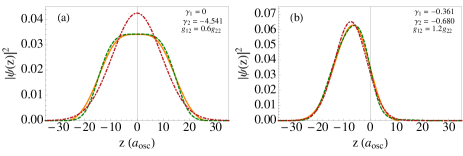
Figure 6: The solid orange curve is the approximate $|\psi_{2}|^{2}$ of the TBEC with $N_{1}=N_{2}=10,000,~{}a_{\text{osc}}=9.566\times 10^{-7},~{}g_{11}=0.553,~{}\text{and}~{}g_{22}=2g_{11}$, obtained by fitting Gram-Charlier A series over numerically obtained density profile (dashed dark-green curve). In (a)$g_{12}=0.6g_{22}$, while in (b) $g_{12}=1.2g_{22}$. The dot-dashed reddish brown shows the density profile of normal distribution with respect to which $\gamma_{1}$ and $\gamma_{2}$ of numerical density profile have been calculated. For first figure, the variational parameters $f$, $c$, $\delta$, and $d$ are $0.177,~{}0.001~{},0~{},~{}8.675$, respectively; while Gram-Charlier values are $0.185,~{}0,~{}0,13.2836$, respectively. For second figure, semi-analytic values of $f$, $c$, $\delta$, and $d$ are $0.267,~{}0,~{}8.529,~{}9.567$,respectively; while Gram-Charlier values are $0.270,~{}0,~{}7.358,~{}8.662$, respectively.

For example, Fig.(6) shows the results of Gram-Charlier analysis of density profile for the second component of the TBEC in miscible and immiscible domains. As is evident from the figure, in the miscible domain, density profile (solid-orange curve) is symmetric and relatively flatter (platykurtic) compared to normal distribution (dot-dashed reddish-brown curve) about origin, and consequently it has zero skewness and negative kurtosis; whereas in second figure, the density distribution has a longer right tail (quantified by positive skewness) and narrow distribution about the mean (leptokurtic) as compared to normal distribution. From Gram-Charlier analysis, we can extract the coefficient of $z^{4}$ (excluding exponential part) and compare it with semi-analytic values of $c^{2}$. For both the cases in Fig.(6), the two values are same up to second decimal place.

III TBECs in optical lattices

In this section, we analyze the ground state geometry of TBECs in optical lattices with the ansatz we have introduced. For this, we consider the optical lattice potential, generated by a pair of orthogonally polarized counter propagating laser beams along axial direction, in presence of the axisymmetric harmonic trapping potential. The period of the lattice potential is half of the laser wavelength. The net external potential experienced by TBEC (in scaled units) is the sum total of the two potentials,

$$V_{i}(r,z)=\frac{1}{2}(r^{2}+\alpha_{i}^{2}z^{2})+V_{0}\cos^{2}\left(\frac{2\pi z}{\lambda}\right),$$ (40)

where $V_{0}=sE_{r}$ is the depth of potential well at each lattice site and $\lambda$ is the wavelength of the laser. Here, $E_{r}=(2\pi/\lambda)^{2}/2$ is the recoil energy of laser light photon and $s$ is the lattice depth scaling parameter. As in the previous section, in weakly interacting regime, the TBEC in cigar shaped traps is like a quasi-1D system and its energy is given by Eq.(17). The axial trapping potential is

$$V_{i}^{a}(z)=\frac{\alpha^{2}z^{2}}{2}+V_{0}\cos^{2}\left(\frac{2\pi z}{\lambda}\right)$$ (41)

In tight binding approximation Trombettoni

$$\psi_{i}(z)=\sqrt{N_{i}}\sum_{n}\zeta_{i}(n)\phi_{n}(z),$$ (42)

where $n$ is index of lattice sites, $\phi_{n}(z)=\phi(z-n\lambda/2-\lambda/4)$ is the wave function with amplitude $\zeta(n)$ localized at $n$th lattice site. Using the tight binding ansatz, energy functional of a TBEC in optical lattice is

$$E = \sum_{n}\left\{\sum_{i=1}^{2}\bigg{[}-2KN_{i}\zeta_{i}(n)\zeta_{i}(n+1)+\epsilon(n)N_{i}|\zeta_{i}(n)|^{2}+\right.$$ (43)

$$\left.\left.\frac{\Lambda_{ii}}{2}N_{i}|\zeta_{i}(n)|^{4}\right]+\Lambda_{12}N_{1}|\zeta_{1}(n)|^{2}|\zeta_{2}(n)|^{2}\right\},$$

where $\Lambda_{ii},~{}\Lambda_{12},~{}K$ and $\epsilon(n)$ are defined as

$$\Lambda_{ii} = 2a_{ii}N_{i}\int\phi_{n}^{4}dz,$$

$$\Lambda_{12} = 2a_{12}N_{2}\int\phi_{n}^{4}dz,$$

$$K = -\int\left[\frac{1}{2}\nabla_{z}\phi_{n}\cdot\nabla_{z}\phi_{n+1}+\phi_{n}V_{i}^{a}(z)\phi_{n+1}\right]dz,$$

$$\epsilon(n) = \int\left[\frac{1}{2}(\nabla_{z}\phi_{n})^{2}+V_{i}^{a}(z)\phi_{n}^{2}\right]dz.$$ (44)

To examine the stationary state of the system we consider $\zeta_{i}(n)$ is real while deriving above relation.

III.1 Ground state

In the weakly interacting regime, the localized wave function $\phi_{n}$ can be taken as ground state wave function of the lattice site,

$$\phi_{n}(z)=\frac{1}{\pi^{1/4}\sqrt{\sigma}}e^{-(z-n\lambda/2-\lambda/4)/(2\sigma^{2})},$$ (45)

where $\sigma=\sqrt{\lambda}/(8\pi^{2}V_{0})^{1/4}$. Ideally, the energy associated with each individual lattice sites can be minimized to evaluate $\phi_{n}(z)$. Neglecting the energy due to harmonic trapping potential and interaction energy in comparison to potential energy due to optical lattice potential, the energy of the $n$th lattice site is approximately

$$\int\left\{\frac{1}{2}\left(\frac{d\phi_{n}}{dz}\right)^{2}+V_{0}\left(\frac{2\pi}{\lambda}\right)^{2}\left[x-\frac{\lambda}{4}(2n+1)\right]^{2}\right\}dz,$$ (46)

where we have used $V_{0}\cos^{2}(2\pi z/\lambda)\approx V_{0}(2\pi/\lambda)^{2}(z-n\lambda/2-\lambda/4)^{2}$ as the potential at the $n$th lattice site. The expressions for $\epsilon(n)$ and $K$ are

$$\epsilon(n) = \frac{V_{0}}{2}\left(1-e^{-\frac{4\pi^{2}\sigma^{2}}{\lambda^{2}}}\right)+\frac{1}{32\sigma^{2}}\left[8+8\alpha^{2}\sigma^{4}\right.$$ (47)

$$\left.+\alpha^{2}\sigma^{2}\lambda^{2}(1+2n)^{2}\right],$$

$$K = -e^{-\frac{\lambda^{2}}{16\sigma^{2}}}\bigg{\{}\frac{V_{0}}{2}\left(1+e^{-\frac{4\pi^{2}\sigma^{2}}{\lambda^{2}}}\right)+\frac{1}{32\sigma^{4}}\left[4\sigma^{4}\lambda^{2}\alpha^{2}\right.$$ (48)

$$\left.\times(1+n)^{2}-\lambda^{2}+8(\sigma^{2}+\alpha^{2}\sigma^{6})\right]\bigg{\}}.$$

Similarly, the energy per boson $\bar{E}=E/(N_{1}+N_{2})$ can be calculated, however, as to be expected the expression is complicated and long. Following our ansatz, we consider

$$\zeta_{1}(n) = ae^{-(n-\gamma)^{2}/(2b^{2})},$$

$$\zeta_{2}(n) = (f+cn^{2})e^{-(n+\delta)^{2}/(2d^{2})},$$ (49)

as the envelope profiles with five independent parameters. The length scale associated with the lattice potential, in scaled units, is $a_{\rm latt}=\sqrt{\omega/\omega_{l}}$, where $\omega_{l}$ is the laser frequency of the optical lattice. Considering that the frequency of the harmonic trapping potential $\omega$ is at the most Khz and $\omega_{l}$ is in the optical region $a_{\rm latt}\ll 1$. Hence, there are large number of lattice sites within the envelope profile. This implies that $b\gg\sigma$ and $d\gg\sigma$, where $\sigma$ is the width of the lattice ground state $\phi_{n}$. We can replace summation over lattice sites with integration over the same variable in Eq.(43). In fact, due to very weak trapping along axial direction, $b$ and $d$ are of the order of a few $a_{\rm osc}$ even for very weak non-linearities. It implies that $e^{-\pi^{2}b^{2}}\rightarrow 0$ and $e^{-\pi^{2}d^{2}}\rightarrow 0$, and in this limit the error incurred in replacing summation by integration approaches zero. From Eq.(43), Eq.(44), and Eq.(49), we calculate the energy per particle which can be minimized to determine the variational parameters. The typical variational results for equal number of atoms of two species are shown in Fig.(11).

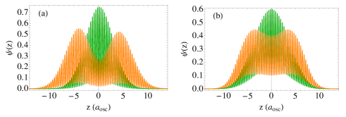
Figure 7: The stationary state solution of the TBEC with $N_{1}=N_{2}=10,000$, $g_{11}=0.465$, $g_{22}=2g_{11}$, $g_{12}=g_{21}=0.8g_{22}$, $\alpha=9/92$, $a_{\rm osc}=1.137\times 10^{-6}m$, $\tilde{\lambda}=0.7$, and $s=6.0$ as the non-linearity and trapping potential parameters, respectively. The criterion, $N_{j}a_{ij}/a_{osc}=g_{ij}/2\sim 1$, for the applicability of the variational ansatz is clearly satisfied. The left and right figures are, respectively, the profiles obtained by variational minimization and numerically solving quasi-1D GP equation.

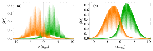
Figure 8: The stationary state solution of the TBEC with $N_{1}=N_{2}=5,000$, $g_{11}=0.233$, $g_{22}=2g_{11}$, $g_{12}=g_{21}=2g_{22}$, $\alpha=9/92$, $a_{\rm osc}=1.137\times 10^{-6}m$, $\tilde{\lambda}=0.7$, and $s=6.0$ as the non-linearity and trapping potential parameters, respectively. The criterion, $N_{j}a_{ij}/a_{osc}=g_{ij}/2\sim 1$, for the applicability of the variational ansatz is clearly satisfied. The left and right figures are, respectively, the profiles obtained by variational minimization and numerically solving quasi-1D GP equation.

Symmetric and Non-symmetric Profiles

Similar to TBECs in harmonic trapping potentials, ground sate geometry of binary condensates in optical lattices can be symmetric or asymmetric. In miscible and weakly segregated domain ( coherence length of the first component is smaller than the penetration depth of the second component Ao ), the ground state geometries are symmetric. For example, a typical symmetric ground state geometry of TBEC in quasi-1D optical lattice is shown in Fig.(7).

In strongly segregated domain ( coherence length of the first component is greater than the penetration depth of the second component), the ground state geometries can be asymmetric. A typical asymmetric ground state geometry of TBEC in quasi-1D optical lattice is shown in Fig.(8).

III.2 Profile narrowing with lattice depth

The density profiles of the two components in TBEC is more compact with deeper lattice potential. To analyze this, we consider an ideal Bose gas ( non-interacting ) trapped in a triple 1D potential well superimposed with a weak harmonic potential

$$V(x)=\left\{\begin{aligned} &\frac{1}{2}\alpha^{2}x^{2}+\frac{1}{2}\beta^{2}(x+d)^{2}&&\text{if }-\frac{3d}{2}\leqslant x<-\frac{d}{2},\\ &\frac{1}{2}\alpha^{2}x^{2}+\frac{1}{2}\beta^{2}x^{2}&&\text{if }-\frac{d}{2}\leqslant x\leqslant\frac{d}{2},\\ &\frac{1}{2}\alpha^{2}x^{2}+\frac{1}{2}\beta^{2}(x-d)^{2}&&\text{if }\frac{d}{2}<x\leqslant\frac{3d}{2},\\ &\infty&&\text{if }|x|>3d/2,\end{aligned}\right.$$ (50)

where $\alpha$ and $\beta$ are the parameters of harmonic and periodic potentials, respectively, and $d$ is the spatial extent of each well. This is most basic model to examine the nearest neighbour effects in a lattice. The central well, in particular, which has two nearest neighbours is a representation of lattice sites in optical lattices. In the experiment set up used by Cataliotti et. al. Cataliotti , the trap geometry is quasi-1D with $\omega_{z}/\omega_{r}=9/92$. For further analysis the equations are scaled in terms of the transverse oscillator length of the harmonic potential realized in aforementioned experimental set up, which is equivalent to setting $\alpha=9/92$. Accordingly, $\beta$ and all the coordinates, from here after, are in scaled units. The potential considered is a simplified model and discontinuities are present at the boundary of two neighbouring wells. However, the ground state energy is much lower than the barrier height and it describes the underlying physics very well. In the tight-binding approximation, the total wave function is

$$\psi(x)=\sum_{i=-1}^{1}a_{i}\phi_{i}(x),$$ (51)

where $i=-1,0,\text{and }1$ represent the left, central, and right well, respectively. Here the normalization is

$$\int_{\infty}^{\infty}|\psi(x)|^{2}dx=1.$$ (52)

We consider $\beta>\alpha$, which follows from the tight binding approximation. The width of each of these localized wave functions are calculated by minimizing the localized energies of each well

$$E_{i}=\int N_{i}\left[\frac{1}{2}|\nabla\phi_{i}|^{2}+V_{i}(x)|\phi_{i}|^{2}\right]dx,$$ (53)

where, from the previous definition

$$V_{i}(x)=\frac{1}{2}x^{2}+\frac{1}{2}\beta^{2}(id+x)^{2}.$$ (54)

The range of each well, as defined earlier, is $(2i-1)d/2\leqslant x\leqslant(2i+1)d/2$. Neglecting the nearest neighbour overlaps of wave the functions, the integration limits can be considered as $-\infty$ to $+\infty$. The energies are then

$$E_{0} = \frac{1}{2}\eta,$$

$$E_{\pm 1} = E_{0}+\delta E$$ (55)

where $\eta=\sqrt{\alpha^{2}+\beta^{2}}$ and

$$\delta E=\frac{\alpha^{2}d^{2}}{2},$$ (56)

is the energy difference between side and central wells.

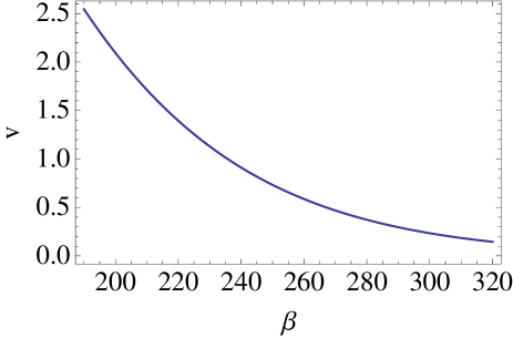
Figure 9: Variation of $v$ as a function of $\beta$.

For the combined system of the three wells, in tight binding approximation, we only consider tunneling between adjacent wells. The lowest eigen energy is the chemical potential of the system and the eigen vector correspond to the probability amplitudes for the occupancy of each well. As defined earlier, $E_{-1}$, $E_{0}$, and $E_{1}$ are the energies localized in left, central, and right well, respectively. Define the tunneling matrix element between left and central well as

$$v=\int\left[\frac{1}{2}\nabla\phi_{-1}\cdot\nabla\phi_{0}+\phi_{-1}V(x)\phi_{0}\right]dx,$$ (57)

and similarly, for the central and right wells as

$$w=\int\left[\frac{1}{2}\nabla\phi_{0}\cdot\nabla\phi_{1}+\phi_{0}V(x)\phi_{1}\right]dx.$$ (58)

For the symmetric case considered here $v=w$, and after evaluating the integrals

$$v = \frac{e^{-\frac{17}{4}d^{2}\eta}}{16\sqrt{\pi\eta}}\bigg{\{}4d\left[\beta^{2}\left(1-2e^{3d^{2}\eta}-2e^{4d^{2}\eta}\right)-\left(1+2e^{3d^{2}\eta}\right)\right]$$ (59)

$$-\sqrt{\pi\eta}e^{4d^{2}\eta}\left[2\eta+d^{2}(5\beta^{2}-3)\right]\text{Erf}\left(d\sqrt{\eta}\right)$$

$$-\sqrt{\pi\eta}e^{4d^{2}\eta}\left[2\eta-d^{2}(11\beta^{2}+3)\right]\text{Erf}\left(2d\sqrt{\eta}\right)\bigg{\}}$$

In the above expression $\text{Erf}(\cdots)$ represents error function. The Hamiltonian matrix of the system is then

$$H=\begin{pmatrix}E_{-1}&v&0\\ v&E_{0}&v\\ 0&v&E_{1}\end{pmatrix}.$$ (60)

The ground state of the system is the lowest energy eigen vector obtained from diagonalizing the Hamiltonian matrix. This is equivalent to solving the secular equation and amounts to calculating the roots of a cubic polynomial, which is possible analytically. The eigen values, in increasing order of magnitude, of the Hamiltonian in Eq.(60) are

$$\frac{1}{2}(E_{0}+E_{1}-E_{12}),~{}~{}E_{1},~{}~{}\frac{1}{2}(E_{0}+E_{1}+E_{12});$$ (61)

where $E_{12}=\sqrt{{\delta E}^{2}+8v^{2}}$. The eigen vector of the lowest eigen value is

$$a_{\pm 1} = \frac{\sqrt{2}v}{\sqrt{8v^{2}+\delta E\left(\delta E+E_{12}\right)}},$$

$$a_{0} = -\frac{\sqrt{8v^{2}+\delta E\left(\delta E+E_{12}\right)}}{\sqrt{2}\sqrt{{\delta E}^{2}+8v^{2}}},$$

and the ratio of the probability amplitude of occupancy of central to side well is

$$\frac{|a_{0}|}{|a_{\pm 1}|}=\frac{\delta E(\delta E+E_{12})+8v^{2}}{2v\sqrt{{\delta E}^{2}+8v^{2}}}.$$ (62)

This energy difference $\delta E$ is quite small for small values of $d$. For example based on Ref.Cataliotti , consider $d=0.35$, and $\beta=197.824$. The associated energy difference and tunneling matrix element are $\delta E=0.00049494$ and $v=2.18549$, respectively. Hence, for $\delta E\ll v$, using Taylor series expansion Eq.(62) simplifies to

$$\frac{|a_{0}|}{|a_{\pm 1}|}\approx\sqrt{2}+\frac{\delta E}{2v}.$$ (63)

Since $\delta E$ is independent of $\beta$ and $v$ decreases as $\beta$ is increased (see Fig.(9)), the above ratio is larger with higher values of $\beta$. Using Eq.(63), Fig.(10) shows the variation of ratio of probability of occupancy of central to side wells with respect to $v$. This relation is not valid for very large values of $\beta$ when $\delta E\ll v$ does not hold true.

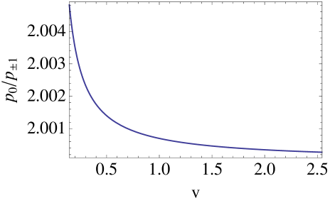
Figure 10: The plot shows the $p_{0}/p_{\pm 1}$ as a function of $v$ for the values of $\beta$ ranging from $197.82$ to $312.79$. In terms of the ratio of barrier height to recoil energy of laser light photon $s$ used in Ref.Cataliotti , the above mentioned range of $\beta$ values is equivalent to $s$ ranging from $6$ to $15$.

For trapping potentials without the harmonic component ($\alpha=0$), purely lattice potential, the three eigenvalues are identical when the hopping across adjacent wells is zero ($v=w=0$). This solution correspond to all the atoms confined to one of the potential wells. At this stage for further reference we define the occupancy probability of the $i$th well as

$$p_{i}=\left(\int_{-\infty}^{\infty}\phi_{i}^{*}\psi dx\right)^{2}=|a_{i}|^{2}.$$ (64)

When $v$ and $w$ are non-zero, then the ground state has nonzero occupancies for all the three wells.The central well has probability of occupancy equal to half ($p_{0}=0.5$) while the wells at the wings have probability equal to one fourth each ($p_{\pm 1}=0.25$). More importantly, these values are are independent of $\beta$. That is, no squeezing of the density profile occurs without the harmonic potential ($\alpha=0$).

In the presence of a weak harmonic potential, there is an increase in $p_{0}$ when $\beta$ is increased. For $\beta=197.82$, equivalent to $s=6$ in Ref.Cataliotti , the occupancy probability of the central well is $0.500047$, this is marginally larger than the $\alpha=0$ case. On the other hand, the wings have occupancy probability of $0.249976$, slightly lower probability of occupancy than $\alpha=0$ case. The trend continues with further increase of $\beta$, and for $\beta=1000$ there are almost no atoms in the potential wells at the wings. Thus with increase in value of $\beta$, atoms migrate from the wings to central well and lead to the squeezing of the condensate. The squeezing of the condensate profile is evident from the comparative study of plots in Fig(11).

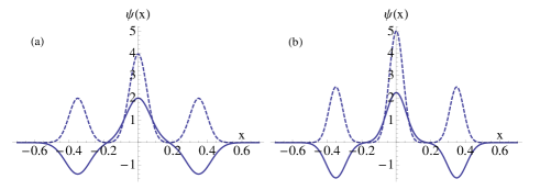
Figure 11: The plots show the ground state wave function $\psi(x)$ (solid curve) and probability density $|\psi(x)|^{2}$ (dashed curve) for potential considered in Eq.(50) For figure on left side, $\alpha=9/92,d=0.35$ and $\beta=197.82$ ($s=6$), while for figure on right side, $\alpha=9/92,d=0.35$ and $\beta=312.79$ ($s=15$)

In three level approximation, a triple well problem can also be analyzed by considering the following classical Hamiltonian Graefe

$$\mathcal{H} = \frac{1}{2}g\left[n_{-1}^{2}+(1-n_{-1}-n_{1})^{2}+n_{1}^{2}\right]+n_{-1}\epsilon_{-1}+n_{1}\epsilon_{1}+$$ (65)

$$2\sqrt{1-n_{-1}-n_{1}}\left(v\sqrt{n_{-1}}\cos\theta_{-1}+w\sqrt{n_{1}}\cos\theta_{1}\right),$$

where $n_{j}=|a_{j}|^{2}$ and $\theta_{j}=\arg(a_{2})-\arg(a_{j})$ are canonical conjugate variables satisfying following equations

$$\frac{dn_{j}}{dt}=-\frac{\partial\mathcal{H}}{\partial\theta_{j}}~{}\text{and}~{}\frac{d\theta_{j}}{dt}=\frac{\partial\mathcal{H}}{\partial n_{j}},$$ (66)

and $\epsilon_{-1}$ and $\epsilon_{1}$ are the zero point energies of potential wells at the flanks measured with respect to zero point energy of central well. The stationary states of the system can be calculated by by solving

$$\frac{dn_{j}}{dt}=\frac{d\theta_{j}}{dt}=0$$ (67)

In the absence of the harmonic potential $\epsilon_{-1}$ and $\epsilon_{1}$ are zero and change in tunneling amplitude has no effect on the occupancy of three wells. But the situation is dramatically different with the harmonic potential, $\epsilon_{-1}=\epsilon_{1}\neq 0$. In this case probability of occupancy of central well increases with decrease in $v$. This is experimentally realizable by increasing depth of lattice potential. Similarly for four potential wells, the occupancy of the two central wells (whose occupancies are equal) grows as we increase $\beta$ for non zero $\alpha$.

IV Conclusions

We have studied the stationary state properties of the TBECs both in miscible and imiscible domains using a variational ansatz. The stationary state geometries obtained using the variational ansatz are in very good agreement with numerical results, especially for very weakly interacting TBECs, i.e., $Na/a_{osc}$ is of the order $1$. We have also quantified the departure of the variational ansatz based semi-analytic results from the numerical ones using Gram-Charlier analysis. Besides harmonic trapping potentials, the present ansatz can also be used to study the TBECs in deep optical lattices where coupled GP equations can be mapped into coupled discrete non-linear Schrödinger equations. In optical lattices, the density profiles of the component species of the TBEC get squeezed with the increase in the height of the potential barrier between adjacent wells. We have explained this phenomenon using a very simple triple well potential model.

V Appendix

$$E_{1}=\frac{\sqrt{\pi}N_{1}}{4}\biggl{[}\frac{a^{2}}{b}+a^{2}b\alpha^{2}(b^{2}+\gamma^{2})+\sqrt{2}a^{4}bg_{11}\biggr{]}$$ (68)

$$E_{2} = \frac{\sqrt{\pi}N_{2}}{1024}\biggl{\{}\frac{64}{d}\bigl{[}4f^{2}-4cf(d^{2}-2\delta^{2})+c^{2}(7d^{4}\bigr{.}\biggr{.}$$ (69)

$$\bigl{.}+20d^{2}\delta^{2}+4\delta^{4})\bigr{]}+64d\bigl{[}4f^{2}(d^{2}+2\delta^{2})+4cf(3d^{4}\bigr{.}$$

$$+12d^{2}\delta^{2}+4\delta^{4})+c^{2}(15d^{6}+90d^{4}\delta^{2}+60d^{2}\delta^{4}$$

$$\bigl{.}+8\delta^{6})\bigr{]}\alpha^{2}+\sqrt{2}d\bigl{[}256f^{4}+256cf^{3}(d^{2}+4\delta^{2})\bigr{.}$$

$$+96c^{2}f^{2}(3d^{4}+24d^{2}\delta^{2}+16\delta^{4})+16c^{3}f(15d^{6}$$

$$\biggl{.}\bigl{.}+180d^{4}\delta^{2}+240d^{2}\delta^{4}+64\delta^{6})+c^{4}(105d^{8}+1680d^{6}\delta^{2}$$

$$+3360d^{4}\delta^{4}+1792d^{2}\delta^{6}+256\delta^{8})\bigr{]}g_{22}\biggr{\}}$$

$$E_{12} = \frac{\sqrt{\pi}a^{2}bdN_{1}g_{12}e^{-\frac{(\gamma+\delta)^{2}}{b^{2}+d^{2}}}}{4(b^{2}+d^{2})^{9/2}}\left\{4d^{8}(f+c\gamma^{2})^{2}\right.$$ (70)

$$+4b^{2}d^{6}\left[4f^{2}+cf(d^{2}+4\gamma^{2}-4\gamma\delta)+c^{2}\gamma^{2}(3d^{2}\right.$$

$$\left.-4\gamma\delta)\right]+b^{8}\left[4f^{2}+4cf(d^{2}+2\delta^{2})+c^{2}(3d^{4}+12d^{2}\delta^{2}\right.$$

$$\left.+4\delta^{4})\right]+2b^{6}d^{2}\left[8f^{2}+c^{2}(3d^{4}-8\gamma\delta^{3}-12d^{2}\delta\gamma\right.$$

$$\left.+6d^{2}\delta^{2})+2cf(3d^{2}-4\delta\gamma+4\delta^{2})\right]+b^{4}d^{4}\left[24f^{2}\right.$$

$$+3c^{2}(d^{4}+4d^{2}\gamma^{2}-8d^{2}\gamma\delta+8\gamma^{2}\delta^{2})+4cf(3d^{2}$$

$$\left.\left.+2\gamma^{2}-8\gamma\delta+2\delta^{2})\right]\right\}$$

$$c = \frac{2}{3d^{5}+12d^{3}\delta^{2}+4d\delta^{4}}\left[-d^{3}f-2df\delta^{2}+\frac{1}{\sqrt{\pi}}\left(3d^{5}\sqrt{\pi}\;\;\;\;\;\right.\right.$$ (71)

$$\biggl{.}\left.-2d^{6}f^{2}\pi+12d^{3}\sqrt{\pi}\delta^{2}-8d^{4}f^{2}\pi\delta^{2}+4d\sqrt{\pi}\delta^{4}\right)^{1/2}\biggr{]}$$