Coherent Nonlinear Single Molecule Microscopy

Abstract

We investigate a nonlinear localization microscopy method based on Rabi oscillations of single emitters. We demonstrate the fundamental working principle of this new technique using a cryogenic far-field experiment in which subwavelength features smaller than $\lambda$/10 are obtained. Using Monte Carlo simulations, we show the superior localization accuracy of this method under realistic conditions and a potential for higher acquisition speed or a lower number of required photons as compared to conventional linear schemes. The method can be adapted to other emitters than molecules and allows for the localization of several emitters at different distances to a single measurement pixel.

Optical microscopy has experienced many revolutionary developments in the past two decades such as scanning near-field optical microscopy (SNOM) Pohl et al. (1984); Lewis et al. (1984), two-photon confocal microscopy, coherent antistokes Raman scattering (CARS) Zumbusch et al. (1999), stimulated emission depletion (STED) Hell (2007), and single-molecule localization microscopy Betzig (1995); Pertsinidis et al. (2010). One of the highest three-dimensional spatial resolution achieved so far has reached about 2 nm Hettich et al. (2002) and was based on the latter concept, where the locations of individual molecules are determined by finding the centers of their diffraction-limited point-spread functions Bobroff (1986); Thompson et al. (2002). The requirement for this technique is the distinguishability of neighboring molecules so that each point-spread function can be examined separately. The first demonstration of this concept was at low temperature Hettich et al. (2002), where the inhomogeneous distribution of frequencies in the sample provides a convenient “spectral identity” for each molecule. More recent approaches have used stochastic photo-activation or switching schemes for addressing single molecules Betzig et al. (2006); Rust et al. (2006). These room-temperature experiments have caused a great deal of interest for their applicability to biological systems, but their accuracy is limited by the number of recorded photocycles before a single molecule undergoes photobleaching.

In this article, we discuss a new scheme of nonlinear localization microscopy based on the observation of coherent Rabi oscillations Gerhardt et al. (2009). In addition to a first experimental demonstration, we present Monte-Carlo simulations and examine the attainable localization accuracy as a function of the number of recorded photons, pixel size, and number of Rabi oscillations. In particular, we compare the performance of coherent Rabi imaging microscopy (CORIM) with standard localization methods, where the spatial distribution of the point-spread function depends linearly on the signal intensity.

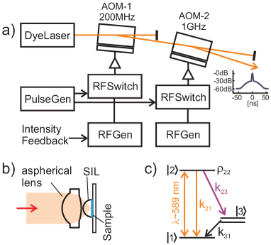
Figure 1: (a) Experimental setup with two cascaded acousto-optical modulators to obtain short laser pulses with a high signal to background ratio. (b) The optical setup inside the cryostat with a solid-immersion lens (SIL). (c) The level scheme of a single molecule.

.1 Experimental localization of a single molecule via position-dependent Rabi oscillations

In this work we studied the dye molecule dibenzantanthrene (DBATT) embedded in a n-tetradecane Shpol’skí matrix. The excited state in DBATT has a fluorescence lifetime of $T_{1}=9.5$ ns, corresponding to a radiatively broadened linewidth of $\mathit{\Gamma}_{1}/2\pi=17$ MHz for the zero phonon line (ZPL) transition. We used a CW single-mode dye laser (Coherent 899 Autoscan, $\Delta\nu\leq 1\,{\rm MHz}$) to identify single molecules via fluorescence excitation spectroscopy Orrit and Bernard (1990). For all further experiments we chopped the beam by means of two cascaded acousto optical modulators (AOMs), achieving pulse width down to 2.9 ns and a signal to background ratio of more than 60 dB. Further details of the pulse generation scheme are explained in a previous publication Gerhardt et al. (2009). As sketched in Fig. 1b, a confocal microscope based on a solid-immersion lens enabled us to efficiently excite a molecule and detect it both via its Stokes-shifted fluorescence and via extinction spectroscopy Wrigge et al. (2008). The red-shifted fluorescence was filtered from the excitation laser light by an optical long pass filter and was detected using an avalanche photodiode (APD).

In coherent state preparation, the system can undergo several Rabi cycles, depending on the pulse area ($A$) which is proportional to the square root of the intensity and the duration of the excitation pulse. Figure 2 shows the experimental results for the integrated Stokes-shifted optical response of a single molecule excited by a series of 4 ns long narrow-band pulses. The signal was averaged for 100 ms and is plotted against the excitation intensity, depicted on a quadratic scale. We note in passing that as illustrated by the dotted line in Fig. 2, a purely linear response as used in conventional localization techniques would appear as a quadratic function in this plot.

If the focal spot of the excitation beam is scanned over the sample, the single emitter experiences different values of $A$ at various lateral coordinates, and the emitted fluorescence signal appears as several concentric rings. The width of each ring depends on the gradient of the intensity at that point and is the smallest at the highest slope of the optical point-spread function. The center of the acquired image depends on the maximum excitation intensity of the molecule and corresponds to several excitation and de-excitation cycles of the emitter. Figures 3a and b show the experimental results of such a measurement on a single molecule with continuous-wave (CW) and pulsed excitations, respectively. The occasional dark regions in the CW image reveal typical triplet-state blinking, while the full width at half-maximum (FWHM) of 370 nm indicates an almost diffraction-limited focusing spot.

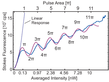
Figure 2: Intensity dependence of the response from a single molecule in temporally integrated detection. Pulse duration was 4 ns, repetition rate was 700 kHz, and the intensity was integrated over 100 ms. Figure adapted from Gerhardt et al. (2009).

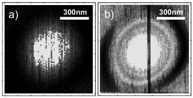
Figure 3: Experimental raster-scanned images of a single molecule without (a) and with (b) pulsed excitation (4 ns pulses, 700 kHz repetition rate). The effectively larger point-spread function of the illumination spot due to the field dependence is visible. The rings around the central spot have widths of $\approx$ 40 nm.

The raster-scanned image with pulsed excitation displays higher spatial frequencies and spatial features down to $\approx$ 40 nm. The dark stripe in the middle of the image was caused by a temporary spectral jump of the molecular resonance and provides a convenient measure for the background fluorescence. We also note the asymmetry of the images in Fig. 3, which might be caused by a cushion distortion slightly away from the optical axis of the solid-immersion lens Ippolito et al. (2005).

.2 Analytical considerations

In Fig. 4a, we first consider the simulated linear response $\widetilde{P}_{red}\propto I_{laser}$ of a single molecule, where $P_{red}$ denotes the red-shifted fluorescence signal. One can localize the molecule as is common in conventional localization schemes by applying a numerical regression to an assumed Gaussian intensity distribution Bobroff (1986); Thompson et al. (2002). The highest spatial frequency in this imaging configuration is given by the diffraction-limited profile of the laser beam focus.

We now consider coherent excitation with light pulses short compared to the lifetime, $t_{p}\ll T_{1}$. Under this condition, the molecular polarization and the population of the ground and excited states oscillate at the Rabi frequency

$${\mathit{\Omega}}=dE(x_{0},y_{0})/\hbar$$ (1)

where $E(x_{0},y_{0})$ is the electric laser field at the position $\{x_{0},y_{0}\}$ of the molecule and $d$ is the transition dipole moment in the direction of the field. The state at the end of the pulse is determined by the pulse area which for a rectangular pulse shape reads

$$A={\mathit{\Omega}}t_{p}\propto\sqrt{I_{laser}}.$$ (2)

As a result, the excited-state population at the end of the pulse follows a sinusoidal shape with increasing $A$. Accordingly, the emission probability of a photon per pulse is given by

$$P=\left(\sin A/2\right)^{2}.$$ (3)

Assuming a Gaussian focal shape, the electric field reads

$$E(x_{0},y_{0})=E_{0}e^{-\left[(x-x_{0})^{2}+(y-y_{0})^{2}\right]/(2w_{0}^{2})}$$ (4)

where $\{x,y\}$ is the position of the focal spot which is scanned over the $x$-$y$ plane. The parameter $w_{0}$ gives the characteristic width of the Gaussian shape. Thus, finds the photon-emission probability to be

$$P=\sin^{2}(f\sqrt{I_{0}}e^{-\left[(x-x_{0})^{2}+(y-y_{0})^{2}\right]/(2w_{0}^{2})})$$ (5)

where $I_{0}$ is the light intensity at the focal spot and $f$ is a scaling parameter. In what follows, we use this expression for the Monte-Carlo simulations.

Experimental measurements such as those in Fig. 3 might deviate from the ideal response. Usually the observed Rabi oscillations might be damped for three reasons: a) a finite pulse length and the dephasing time $T_{2}$ reduce the modulation depth below unity, b) due to the finite pulse length, the molecule decays and is re-excited within the pulse duration several times, and c) the pulse area fluctuations wash out the visibility of the integrated signal. These effects are collectively included in the following equations by damping the oscillations with a field-dependent term $a$. Furthermore, we add a linear contribution $b$ to account for the background, which scales roughly linearly with the optical field as experimentally observed in Gerhardt et al. (2009). Also other molecules might spectrally overlap and lead to a background contribution which is then proportional to the excitation intensity, modeled by $c$. Moreover, the intensity-independent pixel noise (i.e. dark counts from a photodetector) can be denoted by $r$. With the above-mentioned parameters it is possible to describe the full optical response in the following form

$$I_{d}=\eta\frac{\sin^{2}\left(f\sqrt{I}\right)}{a\sqrt{I}}+b\sqrt{I}+cI+r$$ (6)

where $\eta$ covers the collection efficiency, pulse repetition rate, and the reduction by filters used to discriminate between laser and fluorescence light. Figures 4b and d show the contributions of the first and second terms on the right-hand side of Eqn. (6).

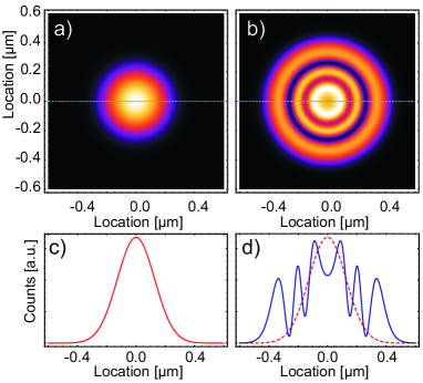
Figure 4: Simulated raster-scanned image of a single molecule and line scans. (a) The usual lineear optical response of a single molecule. (b) If the excitation light is pulsed and the pulse width is shorter than the singlet $T_{\rm 1}$ time of the molecule, several rings appear, representing Rabi oscillations. c, d) Cross sections of (a) and (b).

.3 Monte Carlo analysis of the localization accuracy

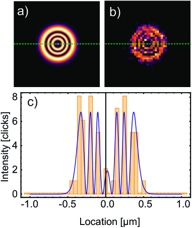
Figure 5: Basic derivation of pixilated images for Monte Carlo estimations: (a) Calculated point-spread function in the absence of amplitude damping and detector noise (analytical). (b) Numerically estimated pixel distribution for 1000 detected photons. (c) Line cuts for pixel distribution and fitted point-spread function.

In order to assess the promise of CORIM for localization microscopy, we performed Monte Carlo simulations using Mathematica 7.01 (Wolfram Research). For realistic experimental parameters, we used a statistical evaluation by generating images followed by a numerical fitting procedure. This method allows us to judge the localization accuracy for a variety of parameters such as the number of detected photons. For each data point and set of parameters, a series of 500 images was generated, by filling a grid of the defined pixel size according to the distribution function (see Fig. 5a) given by Eqn. (5) until the detected number of photons was reached. Figure 5b displays an example of the Monte-Carlo image. The center of the emitter was randomly chosen to be within the inner 2$\times$2 pixel. The pixel grid was defined such that the range around the molecule was larger than 1 $\mu$m by one pixel. The resulting image was fitted by the point-spread function using the Mathematica internal function for nonlinear fitting without any further constraints (NonlinearModelFit). The cross section in Fig. 5c shows an example. Here, experimental background noise has not been included so that only pixilation and shot noise contribute to the observed fluctuations.

The start parameters of the simulations that follow below included the actual center of the spot, the height of the highest pixel as an amplitude, and $w_{0}$ of the optical point-spread function ($w_{0}=\frac{1}{2}\,\mbox{FWHM}/\sqrt{2\ln{2}}\approx$ 120 nm). The 500 Monte Carlo runs were unweighted averaged. The confidence range ($\pm 1~{}\sigma$) of one coordinate is displayed. Unless differently specified, the parameters were as follows: Gaussian focus, FWHM=300 nm, detection of 200 photons, pixel size of 50 nm, and a Rabi parameter of 100, leading to approximately 3 Rabi flops (6.2 $\pi$). These parameters are labeled by the dashed lines in the presented figures.

The localization accuracy with $N$ detected photons scales as 1/$\sqrt{N}$, depending on the shot noise of the measurement. This behavior is observed both for linear imaging and CORIM. At the top of Fig. 6, we show CORIM and Gaussian simulations for different $N$. The bottom part of Fig. 6 summarizes the results and compares the localization error between the two cases. We find that the accuracy in CORIM is superior by a factor of two for the given parameters. Thus, a single emitter can be localized with higher accuracy in a shorter time, which might offer a crucial advantage against systematic errors caused by mechanical drift and jitter Bloeß et al. (2001).

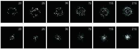
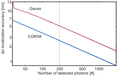
Figure 6: Localization accuracy for different numbers of detected photons. Gaussian fitting (upper red curve) and coherent Rabi imaging microscopy (lower blue curve). Both curves scale as $1/\sqrt{N}$, as expected for pure shot-noise limited localization performance (background noise is neglected in these calculations). For details of this simulation see text.

Linear imaging requires operation below the saturation regime because otherwise the image of a single molecule is distorted with respect to the expected point-spread function. In CORIM, on the other hand, higher intensities simply result in more photo cycles. In fact, the number of Rabi oscillations has a direct impact on the localization accuracy. In Fig. 7 the excitation intensity and thus the number of oscillations are varied. This is realized by changing the pulse area in Eqn. 3. For zero amplitude the CORIM response is equivalent to the linear imaging such that both curves originate at one point. As the number of Rabi oscillations increases, the localization accuracy becomes worse than for Gaussian fitting because of a virtual broadening of the recorded point-spread function. In other words, the same number of photons is distributed unspecifically on a flat-top distribution. However, when the field strength is increased further, the resulting spot is “opened” at the center and the localization accuracy becomes superior to that of a Gaussian fitting. Here, the larger number of observed Rabi oscillations helps to achieve higher spatial frequencies, allowing for better fitting. The slight undulations of the localization accuracy versus the field strength ($E(x_{0},y_{0})$) shows that each time that the optical response opens (this occurs at odd multipliers of $\pi$), the accuracy is improved. The slope of the curve in Fig. 7 yields a $1/\sqrt[4]{E(x_{0},y_{0})}$ behavior for the relative excitation intensity.

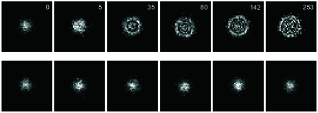
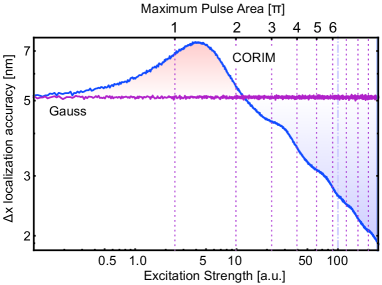
Figure 7: Localization accuracy for Gaussian localization (red curve) and for coherent Rabi imaging microscopy (blue curve). With increasing pulse strength, the Gaussian point-spread function widens first and reduces the localization accuracy by increasing the effective spot size. At an intensity of about 2$\pi$, the localization gets better than linear imaging. The oscillations for higher field strength are explained by opening and closing the inner spot of the point spread function. See text for details on the excitation strength units and the details of the simulation.

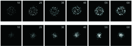
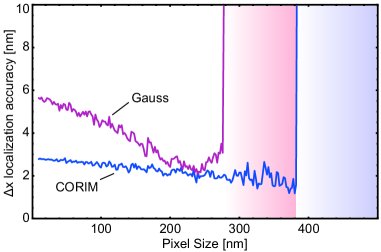
Figure 8: Localization accuracy for different pixel sizes. The coherent Rabi imaging microscopy (blue curve) has a higher stability against fitting. Note that background noise is neglected such that only pixilation noise is present. For details of this simulation see text.

As shown by Thompson and coworkers Thompson et al. (2002), the localization accuracy depends also on the pixel size. In Fig. 8 we present a comparison between linear imaging and CORIM regarding the influence of the pixilation noise on the localization accuracy. We see that in both cases the localization procedure becomes meaningless for large pixels, however CORIM turns out to be more tolerant in this respect.

The decisive parameters in finding the center of an emission spot are the total number of detected photons, the pixel size, and pixilation noise causing higher frequency components in the image Heintzmann and Gustafsson (2009). Besides these factors, any additional source of noise introduces extra error in the localization accuracy. One important omnipresent example stems from the background fluorescence of the sample and other molecules in it. In the case of pulsed excitation two other issues have to be kept in mind. If the pulse has a finite length, there is a certain probability that the single emitter decays and is re-excited within the pulse duration. Furthermore, pulse fluctuations in time and intensity wash out the modulation depth.

While we have chosen to analyze Monte Carlo simulations in this work, a variety of other measures can be used for evaluating the localization accuracy in microscopy Thompson et al. (2002). For example, one could start with the expected point-spread function (see Fig. 5a), add different kinds of noise at each pixel and analyze the localization error. A similar strategy corresponds to the characterization of the Cramer-Rao lower bound by calculating the Fisher information contents Ober et al. (2004). However, regardless of the exact procedure, it is apparent that higher spatial frequencies in the overall point-spread function provide more information and improve the localization accuracy. In particular, the largest slope of the point-spread function contributes most to the localization accuracy Bobroff (1986).

.4 Resolving several emitters

Having discussed the accuracy in the localization of a single molecule, we now explore the potential of CORIM for resolving several close-lying emitters. Since in the experiment we only collect red-shifted incoherent photons, we simply add the amplitudes and do not need to include interferences Scully and Zubairy (1997).

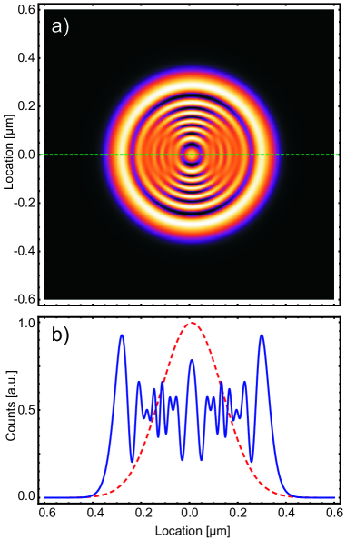
Figure 9: (a) Simulated image of two molecules located at a distance of 20 nm experiencing the same effective pulse area with the same illumination strength. The concentric rings with sub-wavelength features can be easily differentiated. (b) A line cut through the central of the point-spread function.

Figure 9 displays an example of two emitters separated by 20 nm along the x-axis. On the separation axis it is apparent that one maximum of the response coincides with the minimum of the other emitter. The situation is analogous to magnetic resonance imaging (MRI) or super-resolution microscopy in inhomogeneous electric fields Hettich et al. (2002), where externally imposed static field gradients lead to position-dependent spectral shifts. Here the field gradient is provided by an inhomogeneous light intensity distribution. If we consider several concentric rings, we can assign a conservative bound to the localization accuracy by the resulting width of the rings.

Let us start by considering emitters with negligible transition frequency differences. As a concrete example, we assume four close-lying emitters as depicted in Fig. 10a and recorde the Rabi response at a central pixel labeled by a green cross. At this point the emitters feel different effective pulse areas and thus undergo different Rabi frequencies, leading to a complex beating pattern that results if one plots the fluorescence signal as a function of field strength (see Fig. 10b). However, Fig. 10c reveals that the Fourier transform of this signal clearly identifies four Rabi frequencies corresponding to the four molecules separated by a fraction of the wavelength.

If the transition frequencies of the emitters are slightly different (as e.g. in the inhomogeneous band of molecules), it is still possible to address them simultaneously by using an optical pulse that is short enough to cover their frequency differences. If the emitters show a considerable inhomogeneous broadening, the frequency detuning $\Delta$ contributes to the effective Rabi frequency according to $\mathit{\Omega}_{\rm eff}=\sqrt{\mathit{\Omega}^{2}+\mathit{\Delta}^{2}}$. If we now scan the focus across the sample, the Rabi response differs not only because of the effective excitation strength, but also because of the different spectral response. As a result, the asymmetry of the point-spread function is larger than in the earlier case and lateral shifts in the order of 1 nm can be resolved. This also represents a convenient method to locate coupled molecules as it has been observed in Hettich et al. (2002).

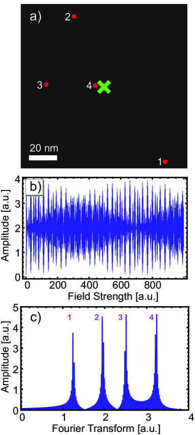
Figure 10: (a) Simulated image of four molecules (red dots), located at a small distance from the measurement point. The field dependence measured on a central pixel (green cross) is displayed in (b). c) The fourier transform of the Rabi oscillations reveal that although measured only at one single pixel, all four emitters can be determined. If the inhomogeneous broadening of the Rabi response is negligible, the distance of all emitters to the measurement spot can be determined.

.5 Outlook

We have introduced a method to localize emitters based on coherent Rabi oscillations. The technique introduces higher spatial frequencies in the recorded images, allowing for a higher localization accuracy with fewer photons. It is possible to extend these experiments to ambient conditions if the coherent features of single molecules are explored further Brinks et al. (2010). Moreover, a single emitter can be used to sample and characterize an optical pulse at nanoscopic scales.

The localization technique discussed here can be readily generalized to other coherently driven processes and emitters. For example, one can apply it to ions in a trap where numerous Rabi oscillations have been demonstrated with a very high fidelity Roos et al. (1999). Furthermore, CORIM can be applied to emitters such as NV- centers in diamond with microwave transitions of the ground state.

.6 Acknowledgements

I.G. acknowledges discussions with A. Walser and M. Badieirostami and continuous support from J. Wrachtrup and F. Jelezko. We thank A. Renn for valuable discussions and advice. This work was financed by the Schweizerische Nationalfond (SNF) and the ETH Zurich initiative for Quantum Systems for Information Technology (QSIT).

References

- Pohl et al. (1984) D. W. Pohl, W. Denk, and M. Lanz, Applied Physics Letters 44, 651 (1984).
- Lewis et al. (1984) A. Lewis, M. Isaacson, A. Harootunian, and A. Muray, Ultramicroscopy 13, 227 (1984).
- Zumbusch et al. (1999) A. Zumbusch, G. R. Holtom, and X. S. Xie, Physical Review Letters 82, 4142 (1999).
- Hell (2007) S. W. Hell, Science 316, 1153 (2007).
- Betzig (1995) E. Betzig, Optics Letters 20, 237 (1995).
- Pertsinidis et al. (2010) A. Pertsinidis, Y. Zhang, and S. Chu, Nature 466, 647 (2010).
- Hettich et al. (2002) C. Hettich, C. Schmitt, J. Zitzmann, S. Kühn, I. Gerhardt, and V. Sandoghdar, Science 298, 385 (2002).
- Bobroff (1986) N. Bobroff, Review of Scientific Instruments 57, 1152 (1986).
- Thompson et al. (2002) R. E. Thompson, D. R. Larson, and W. W. Webb, Biophysical Journal 82, 2775 (2002).
- Betzig et al. (2006) E. Betzig, G. H. Patterson, R. Sougrat, O. W. Lindwasser, S. Olenych, J. S. Bonifacino, M. W. Davidson, J. Lippincott-Schwartz, and H. F. Hess, Science 313, 1642 (2006).
- Rust et al. (2006) M. J. Rust, M. Bates, and X. Zhuang, Nature Methods 3, 793 (2006).
- Gerhardt et al. (2009) I. Gerhardt, G. Wrigge, G. Zumofen, J. Hwang, A. Renn, and V. Sandoghdar, Physical Review A 79, 011402 (2009).
- Orrit and Bernard (1990) M. Orrit and J. Bernard, Physical Review Letters 65, 2716 (1990).
- Wrigge et al. (2008) G. Wrigge, I. Gerhardt, J. Hwang, G. Zumofen, and V. Sandoghdar, Nature Physics 4, 60 (2008).
- Ippolito et al. (2005) S. B. Ippolito, B. B. Goldberg, and M. S. Ünlü, Journal of Applied Physics 97, 053105 (2005).
- Bloeß et al. (2001) A. Bloeß, Y. Durand, M. Matsushita, H. van der Meer, G. J. Brakenhoff, and J. Schmidt, Journal of Microscopy 205, 76 (2001).
- Heintzmann and Gustafsson (2009) R. Heintzmann and M. G. L. Gustafsson, Nature Photonics 3, 362 (2009).
- Ober et al. (2004) R. J. Ober, S. Ram, and E. S. Ward, Biophysical Journal 86, 1185 (2004).
- Scully and Zubairy (1997) M. O. Scully and M. S. Zubairy, Quantum Optics, 1st ed. (Cambridge University Press, 1997).
- Brinks et al. (2010) D. Brinks, F. D. Stefani, F. Kulzer, R. Hildner, T. H. Taminiau, Y. Avlasevich, K. Müllen, and N. F. van Hulst, Nature 465, 905 (2010).
- Roos et al. (1999) C. Roos, T. Zeiger, H. Rohde, H. C. Nägerl, J. Eschner, D. Leibfried, F. Schmidt-Kaler, and R. Blatt, Physical Review Letters 83, 4713 (1999).