A LOCAL BASELINE OF THE BLACK HOLE MASS SCALING RELATIONS FOR ACTIVE GALAXIES. I.
METHODOLOGY AND RESULTS OF PILOT STUDY

Abstract

We present high-quality Keck/LRIS longslit spectroscopy of a pilot sample of 25 local active galaxies selected from the SDSS (0.02 $\leq$ $z$ $\leq$ 0.1; $M_{\rm BH}$$>10^{7}$M_⊙) to study the relations between black hole mass ($M_{\rm BH}$) and host-galaxy properties. We determine stellar kinematics of the host galaxy, deriving stellar-velocity dispersion profiles and rotation curves from three spectral regions (including CaH&K, MgIb triplet, and CaII triplet). In addition, we perform surface photometry on SDSS images, using a newly developed code for joint multi-band analysis. BH masses are estimated from the width of the H$\beta$ emission line and the host-galaxy free 5100Å AGN luminosity. Combining results from spectroscopy and imaging allows us to study four $M_{\rm BH}$ scaling relations: $M_{\rm BH}$-$\sigma$, $M_{\rm BH}$-$L_{\rm sph}$, $M_{\rm BH}$-$M_{\rm sph,\star}$, and $M_{\rm BH}$-$M_{\rm sph,dyn}$. We find the following results. First, stellar-velocity dispersions determined from aperture spectra (e.g. SDSS fiber spectra or unresolved data from distant galaxies) can be biased, depending on aperture size, AGN contamination, and host-galaxy morphology. However, such a bias cannot explain the offset seen in the $M_{\rm BH}$-$\sigma$ relation at higher redshifts. Second, while the CaT region is the cleanest to determine stellar-velocity dispersions, both the MgIb region, corrected for FeII emission, and the CaHK region, although often swamped by the AGN powerlaw continuum and emission lines, can give results accurate to within a few percent. Third, the $M_{\rm BH}$ scaling relations of our pilot sample agree in slope and scatter with those of other local active and inactive galaxies. In the next papers of the series we will quantify the scaling relations, exploiting the full sample of $\sim 100$ objects.

1. INTRODUCTION

The empirical relations between the mass of the central supermassive black hole (BH) and the properties of the spheroid (ellipticals and classical bulges of spirals) such as stellar-velocity dispersion $\sigma$ (Ferrarese & Merritt, 2000; Gebhardt et al., 2000), stellar mass (e.g., Marconi & Hunt, 2003), and luminosity (e.g., Häring & Rix, 2004) discovered in the local Universe have been interpreted as an indication of a close connection between the growth of the BH and the formation and evolution of galaxies (e.g., Kauffmann & Haehnelt, 2000; Volonteri et al., 2003; Ciotti & Ostriker, 2007; Hopkins et al., 2007; Di Matteo et al., 2008; Hopkins et al., 2009). In this framework, active galactic nuclei (AGNs) are thought to represent a stage in the evolution of galaxies in which the supermassive BH is actively growing through accretion.

To understand the origin of the BH mass ($M_{\rm BH}$) scaling relations, our group has been studying their evolution with cosmic time (Treu et al., 2004; Woo et al., 2006; Treu et al., 2007; Woo et al., 2008; Bennert et al., 2010). To distinguish mechanisms causing evolution in $\sigma$ (e.g., dissipational merger events) and $L_{\rm sph}$ (e.g., through passive evolution due to aging of the stellar population, or dissipationless mergers), we simultaneously study both the $M_{\rm BH}$-$\sigma$ and $M_{\rm BH}$-$L_{\rm sph}$ relations for a sample of low-luminous AGNs, Seyfert-1 galaxies, at $z\simeq 0.4$ and 0.6 (lookback time 4-6 Gyrs). Our results reveal an offset with respect to the local relationships which cannot be accounted for by known systematic uncertainties. The evolutionary trend we find (e.g., $M_{\rm BH}$/$L_{\rm sph}$$\propto$ $(1+z)^{1.4\pm 0.2}$, including selection effects; Bennert et al., 2010) suggests that BH growth precedes spheroid assembly. Several other studies have found results in qualitative agreement with ours, over different ranges in black hole mass and redshifts, and with different observing techniques (e.g., Walter et al., 2004; Shields et al., 2006; McLure et al., 2006; Peng et al., 2006b; Salviander et al., 2007; Weiss et al., 2007; Riechers et al., 2008, 2009; Gu et al., 2009; Jahnke et al., 2010; Decarli et al., 2010; Merloni et al., 2010).

However, to study the evolution of the $M_{\rm BH}$ scaling relations, it is crucial to understand slope and scatter of the local relations. In particular, an open question is whether quiescent galaxies and active galaxies follow the same relations, as expected if the nuclear activity was just a transient phase in the life-cycle of galaxies. Recently, Woo et al. (2010) presented the $M_{\rm BH}$-$\sigma$ relation for a sample of 24 active galaxies in the local Universe, for which the BH mass was derived via reverberation mapping (RM) (e.g., Wandel et al., 1999; Kaspi et al., 2000, 2005; Bentz et al., 2006, 2009b). They find a slope ($\beta=3.55\pm 0.60$) and intrinsic scatter ($\sigma_{\rm int}=0.43\pm 0.08$) which are indistinguishable from that of quiescent galaxies (e.g., Ferrarese & Ford, 2005; Gültekin et al., 2009) within the uncertainties, supporting the scenario in which active galaxies are an evolutionary stage in the life cycle of galaxies.

While the great advantage of such a study is the multi-epoch data which provide more reliable measurements of the BH mass, such a quality comes at the expense of quantity. Studies based on larger samples drawn from the Sloan Digital Sky Survey (SDSS) infer the BH mass indirectly from single-epoch spectra (e.g., Greene & Ho, 2006a; Shen et al., 2008). They hinted at a shallower $M_{\rm BH}$-$\sigma$ relation than that observed for quiescent samples, but the available dynamic range is too small to be conclusive. In particular, the relation above 10^7.5 M_⊙ is very poorly known, which has profound implications for evolutionary studies that by necessity focus on this mass range.

However, there is another uncertainty in the $M_{\rm BH}$-$\sigma$ relation that arises when measuring $\sigma$ from fiber-based SDSS data (e.g., Greene & Ho, 2006a; Shen et al., 2008) and also from the unresolved “aperture spectra” for more distant galaxies (e.g., our studies on the evolution of the $M_{\rm BH}$-$\sigma$ relation; Woo et al., 2006, 2008, J.-H. Woo et al. 2011, in preparation). Local active galaxies seem to span a range of morphologies (e.g., Malkan et al., 1998; Hunt & Malkan, 2004; Kim et al., 2008; Bentz et al., 2009a) and a significant fraction ($>$15/40) of our distant sample of Seyfert-1 galaxies have morphologies of Sa or later (Bennert et al., 2010). Given the diversity of morphologies of AGN hosts, it is most likely that there is a degree of rotational support: If the disk is seen edge-on, the disk rotation can bias $\sigma$ towards higher values. However, since the disk is kinematically cold, it can also result in the opposite effect, i.e. biassing $\sigma$ towards smaller values, if the disk is seen face on (e.g., Woo et al., 2006). Either way, it questions the connection between the “global” dispersion measured by those experiments and the spheroid-only dispersion which may in fact scale more tightly with BH mass.

More generally, measuring $\sigma$ in type-1 AGNs is complicated by the presence of strong emission lines and a continuum that dilutes the starlight. $\sigma$ can be measured from different spectral regions with different merits and complications (Greene & Ho, 2006b, for inactive galaxies see also Barth et al. 2002). Finally, there is are different $\sigma$ measurements in use: e.g., the luminosity-weighted line-of-sight velocity dispersion within the spheroid effective radius ($\sigma_{\rm reff}$, e.g., Gebhardt et al., 2000, 2003), and the central velocity dispersions normalized to an aperture of radius equal to 1/8 of the galaxy effective radius ($\sigma_{\rm 1/8reff}$, e.g., Ferrarese & Merritt, 2000; Ferrarese & Ford, 2005).

Shedding light on the issues outlined above is essential to understand what aspects of galaxy formation and AGN activity are connected, but it requires spatially-resolved kinematic information for a large sample of local AGNs. For this purpose, we selected a sample of $\sim$100 local (0.02 $\leq$ $z$ $\leq$ 0.1) Seyfert-1 galaxies from the SDSS (DR6) with $M_{\rm BH}$$>10^{7}$M_⊙ and obtained high-quality longslit spectra with Keck/LRIS. From the Keck spectra, we derive the BH mass and measure the spatially-resolved stellar-velocity dispersion from three different spectral regions (around CaH+K $\lambda\lambda$3969,3934Å; around MgIb $\lambda\lambda\lambda$5167,5173,5184Å triplet; and around Ca II$\lambda\lambda\lambda$8498,8542,8662Å triplet). The spectra are complemented by archival SDSS images (g’, r’, i’, z’) on which we perform surface photometry using a newly developed code to determine the spheroid effective radius, spheroid luminosity, and the host-galaxy free 5100Å luminosity of the AGN (for an accurate BH mass measurement). Our code allows a joint multi-band analysis to disentangle the AGN which dominates in the blue from the host galaxy that dominates in the red. The resulting multi-filter spheroid luminosities allow us to estimate spheroid stellar masses.

Combining the results from spectroscopic and imaging analysis, we can study four different BH mass scaling relations (namely $M_{\rm BH}$-$\sigma$, $M_{\rm BH}$-$L_{\rm sph}$, $M_{\rm BH}$-$M_{\rm sph,\star}$, and $M_{\rm BH}$-$M_{\rm sph,dyn}$). In this paper, we focus on the methodology and present results for a pilot sample of 25 objects. The full sample will be discussed in the upcoming papers of this series. The paper is organized as follows. We summarize sample selection and sample properties in § 2; observations and data reduction in § 3. § 4 describes the derived quantities, such as spatially-resolved stellar-velocity dispersion and velocity, aperture stellar-velocity dispersion, BH masses, surface photometry, and spheroid masses. In § 5, we describe comparison samples drawn from literature, consisting of local inactive and active galaxies. We present and discuss our results in § 6, including the BH mass scaling relations. We conclude with a summary in § 7. In Appendix A, we describe the details of a python-based code developed by us to determine surface-photometry from multi-filter SDSS images. Throughout the paper, we assume a Hubble constant of $H_{0}$ = 70 km s^-1 Mpc^-1, $\Omega_{\Lambda}$ = 0.7 and $\Omega_{\rm M}$ = 0.3.

2. SAMPLE SELECTION

Making use of the SDSS DR6 data release, we selected type-1 AGNs with $M_{\rm BH}$$>10^{7}$M_⊙, as estimated from the spectra based on their optical luminosity and H$\beta$ full-width-at-half-maximum (FWHM) (McGill et al., 2008). We restricted the redshift range to $0.02-0.1$ to ensure that both the Ca triplet and a bluer wavelength region are accessible to measure stellar kinematics and that the objects are well resolved. This results in a list of 332 objects from which targets were selected based on visibility during the assigned Keck observing time. Moreover, we visually inspected all spectra to make sure that the BH mass measurement is reliable and that there are no spurious outliers lacking broad emission lines ($\sim$5% of the objects). A total of 111 objects were observed with Keck between January 2009 and March 2010. Here, we present the methodology of our approach and the results for our pilot sample of 25 objects. Their properties are summarized in Table 1. Fig. 1 shows postage stamp SDSS-DR7 images. The results for the full sample will be presented in the forthcoming papers of this series.

All 25 objects were covered by the VLA FIRST (Faint Images of the Radio Sky at Twenty-cm) survey, but only 10 have detected counterparts within a radius of 5″. Out of these 10, seven are listed in Li et al. (2008) with only one being radio-loud. Thus, the majority ($>$$\sim$85%) of our objects are radio-quiet. Note that none of the objects has HST images available. As our sample was selected from the SDSS, most objects are included in studies that discuss the local BH mass function (Greene & Ho, 2007) or BH fundamental plane (Li et al., 2008). In addition, 1535+5754 (Mrk 290) has a reverberation-mapped BH mass from Denney et al. (2010). We will compare the BH masses derived in these studies with ours when we present the full sample. For a total of eight objects, stellar-velocity dispersion measurements from aperture spectra exist in the literature (mainly derived from SDSS fiber data: six in Greene & Ho 2006a and five in Shen et al. 2008, with three overlapping, and one object in Nelson & Whittle 1996 determined from independent spectra, but included in both SDSS studies). We briefly compare the stellar-velocity dispersions derived in these studies with ours in § 4.2, but will get back to it in more detail when we present the full sample.

Table 1Sample Properties

Object	SDSS Name	$z$	$D_{\rm L}$	Scale	RA (J2000)	DEC (J2000)	$i^{\prime}$	Alternative Name(s)
			(Mpc)	(kpc/arcsec)			(mag)
(1)	(2)	(3)	(4)	(5)	(6)	(7)	(8)	(9)
0121-0102	SDSSJ012159.81-010224.4	0.0540	240.8	1.05	01 21 59.81	-01 02 24.4	14.32	Mrk 1503
0206-0017	SDSSJ020615.98-001729.1	0.0430	190.2	0.85	02 06 15.98	-00 17 29.1	13.24	Mrk 1018, UGC 01597
0353-0623	SDSSJ035301.02-062326.3	0.0760	344.1	1.44	03 53 01.02	-06 23 26.3	16.10
0802+3104	SDSSJ080243.40+310403.3	0.0410	181.1	0.81	08 02 43.40	+31 04 03.3	15.06
0846+2522	SDSSJ084654.09+252212.3	0.0510	226.9	1.00	08 46 54.09	+25 22 12.3	15.16
1042+0414	SDSSJ104252.94+041441.1	0.0524	233.4	1.02	10 42 52.94	+04 14 41.1	15.82
1043+1105	SDSSJ104326.47+110524.2	0.0475	210.8	0.93	10 43 26.47	+11 05 24.3	16.06
1049+2451	SDSSJ104925.39+245123.7	0.0550	245.4	1.07	10 49 25.39	+24 51 23.7	15.52
1101+1102	SDSSJ110101.78+110248.8	0.0355	156.2	0.71	11 01 01.78	+11 02 48.8	14.67	MRK 728
1116+4123	SDSSJ111607.65+412353.2	0.0210	91.4	0.43	11 16 07.65	+41 23 53.2	14.08	UGC 06285
1144+3653	SDSSJ114429.88+365308.5	0.0380	167.5	0.75	11 44 29.88	+36 53 08.5	14.50
1210+3820	SDSSJ121044.27+382010.3	0.0229	99.8	0.46	12 10 44.27	+38 20 10.3	13.89
1250-0249	SDSSJ125042.44-024931.5	0.0470	208.5	0.92	12 50 42.44	-02 49 31.5	14.47
1323+2701	SDSSJ132310.39+270140.4	0.0559	249.6	1.09	13 23 10.39	+27 01 40.4	16.25
1355+3834	SDSSJ135553.52+383428.5	0.0501	222.7	0.98	13 55 53.52	+38 34 28.5	15.72	Mrk 0464
1405-0259	SDSSJ140514.86-025901.2	0.0541	241.2	1.05	14 05 14.86	-02 59 01.2	15.15
1419+0754	SDSSJ141908.30+075449.6	0.0558	249.1	1.08	14 19 08.30	+07 54 49.6	14.01
1434+4839	SDSSJ143452.45+483942.8	0.0365	160.7	0.73	14 34 52.45	+48 39 42.8	14.29	NGC5̇683
1535+5754	SDSSJ153552.40+575409.3	0.0304	133.2	0.61	15 35 52.40	+57 54 09.3	14.52	Mrk 290
1545+1709	SDSSJ154507.53+170951.1	0.0481	213.5	0.94	15 45 07.53	+17 09 51.1	15.66
1554+3238	SDSSJ155417.42+323837.6	0.0483	214.5	0.95	15 54 17.42	+32 38 37.6	14.88
1557+0830	SDSSJ155733.13+083042.9	0.0465	206.2	0.91	15 57 33.13	+08 30 42.9	16.31
1605+3305	SDSSJ160502.46+330544.8	0.0532	237.1	1.04	16 05 02.46	+33 05 44.8	15.66
1606+3324	SDSSJ160655.94+332400.3	0.0585	261.7	1.13	16 06 55.94	+33 24 00.3	15.45
1611+5211	SDSSJ161156.30+521116.8	0.0409	180.6	0.81	16 11 56.30	+52 11 16.8	15.17

Note. — Col. (1): Target ID used throughout the text (based on RA and DEC). Col. (2): Full SDSS name. Col. (3): Redshift from SDSS-DR7. Col. (4): Luminosity distance in Mpc, based on redshift and the adopted cosmology. Col. (5): Scale in kpc/arcsec, based on redshift and the adopted cosmology. Col. (6): Right Ascension. Col. (7): Declination. Col. (8): $i^{\prime}$ AB magnitude from SDSS-DR7 photometry (“modelMag_i”). Col. (9): Alternative name(s) from the NASA/IPAC Extragalactic Database (NED).

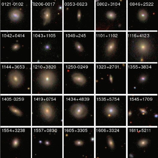
Figure 1.— Postage stamp SDSS-DR7 multi-filter images. North is up, east is to the left. The size of the field-of-view is 50″$\times$50″ (corresponding to $\sim$20$\times$20kpc up to $\sim$76$\times$76kpc for the redshift range covered by the objects presented here). For 0206-0017, we show the central 100″$\times$100″.

3. SPECTROSCOPY: OBSERVATIONS AND DATA REDUCTION

We here summarize only the spectroscopic observations and data reduction. The photometric data consist of SDSS archival images and the data reduction is summarized in Appendix A.

All objects were observed with the Low Resolution Imaging Spectrometer (LRIS) at Keck I, using a 1″ wide longslit, the D560 dichroic, the 600/4000 grism in the blue, and the 831/8200 grating in the red (central wavelength = 8950Å). In addition to inferring the BH mass from the width of the broad H$\beta$ line, this setup allows us to simultaneously cover three spectral regions commonly used to determine stellar-velocity dispersions. In the blue, we cover the region around the CaH+K $\lambda\lambda$3969,3934Å (hereafter CaHK) and around the MgIb $\lambda\lambda\lambda$5167,5173,5184Å triplet (hereafter MgIb); in the red, we cover the Ca II$\lambda\lambda\lambda$8498,8542,8662Å triplet (hereafter CaT). The instrumental spectral resolution is $\sim$90 km s^-1 in the blue and $\sim$45 km s^-1 in the red.

The long slit was aligned with the host galaxy major axis as determined from SDSS (“expPhi_r”), allowing us to measure the stellar-velocity dispersion profile and rotation curves. Observations were carried out on January 21 2009 (clear, seeing 1-1.5″), January 22 2009 (clear, seeing $\sim$1.1″), April 15 2009 (scattered clouds, seeing $\sim$1″), and April 16 2009 (clear, seeing $\sim$0.8″; see also Table 2).

Table 2Details of Observation and Reduction

Object	PA	Exp. time	Date	S/Nblue	S/Nred	FeII sub.
		(sec)
(1)	(2)	(3)	(4)	(5)	(6)	(7)
0121-0102	65.6	1200	01-21-09	111.7	85.8	yes
0206-0017	176.0	1200	01-22-09	152.7	142.8	no
0353-0623	171.2	1200	01-22-09	50.2	40.2	yes
0802+3104	82.9	1200	01-21-09	79.1	72.8	yes
0846+2522	50.9	1200	01-22-09	103.6	89.2	no
1042+0414	126.2	1200	04-16-09	53.8	52.1	yes
1043+1105a	128.2	600	04-16-09	22.9	17.4	no
1049+2451	29.9	600	04-16-09	52.2	43.1	yes
1101+1102	147.5	600	04-16-09	32.2	37.5	yes
1116+4123	11.7	850	04-15-09	46.3	62.4	no
1144+3653	20.7	600	04-16-09	58.7	62.4	no
1210+3820	0.8	600	04-16-09	113.1	132.7	yes
1250-0249	73.9	1200	04-16-09	37.3	45.8	yes
1323+2701	8.1	700	04-16-09	25.0	28.7	no
1355+3834a	78.0	300	04-16-09	34.7	34.4	no
1405-0259	64.8	1600	04-16-09	54.4	72.2	yes
1419+0754	19.3	900	04-16-09	58.8	80.1	yes
1434+4839	152.1	600	04-16-09	49.6	61.3	yes
1535+5754	103.8	1200	04-15-09	180.8	169.6	yes
1545+1709	60.0	1200	04-15-09	83.7	91.3	no
1554+3238	169.1	1200	04-15-09	83.6	95.0	yes
1557+0830a	58.6	1200	04-15-09	54.9	55.6	yes
1605+3305	90.2	1200	04-15-09	80.0	80.9	yes
1606+3324	20.8	1200	04-15-09	44.9	59.1	yes
1611+5211	114.3	1200	04-15-09	72.3	84.4	no

Note. — Col. (1): Target ID. Col. (2): Position angle of major axis, along which the long slit was placed (taken from SDSS-DR7 “expPhi_r”). Col. (3): Total exposure time in seconds. Col. (4): Date of Observations (month-day-year). Col. (5): S/N in total blue spectrum (per pix, at rest wavelength 5050-5450Å), aperture size $\sim$7″. Col. (6): S/N in total red spectrum (per pix, at rest wavelength 8480-8690Å), aperture size $\sim$7″. Col. (7): Subtraction of broad FeII emission.

^a Note that for these three objects, the spectra did not allow a robust measurement of the stellar kinematics due to AGN contamination and we only present BH mass and results from surface photometry.

Note that all data included in this paper were obtained before the LRIS red upgrade. The rest of our sample ($\sim$75 objects) benefited from the upgrade with higher throughput and lower fringing (data obtained from June 2009 onwards) and will be presented in an upcoming paper (C. E. Harris et al. 2011, in preparation). A total of 25 objects were observed with the old red LRIS chip. For three objects, the spectra did not allow a robust measurement of the stellar kinematics, due to dominating AGN continuum and emission lines. However, we were able to determine BH mass and surface photometry. Thus our “imaging” sample consists of 25 objects, our “spectroscopic” sample of 22 objects.

The data were reduced using a python-based script which includes the standard reduction steps such as bias subtraction, flat fielding, and cosmic ray rejection. Arc-lamps were used for wavelength calibration in the blue spectral range, sky emission lines in the red. A0V Hipparcos stars, observed immediately after a group of objects close in coordinates (to minimize overhead), were used to correct for telluric absorption and perform relative flux calibration.

From these final reduced 2D spectra, we extracted 1D spectra in the following manner. For the blue, a central spectrum with a width of 1.08″  (8 pixels) was extracted to measure the H$\beta$ width for BH mass determination, i.e. encompassing the broad-line region (BLR) emission given a typical seeing of $\simeq$1″ and a slit width of 1″. To measure the stellar-velocity dispersion and its variation as a function of radius, we extracted a central spectrum with a width of 0.54″ (0.43″) for the blue (red). Outer spectra were extracted by stepping out in both directions, increasing the width of the extraction window by one pixel at each step (above and below the trace) choosing the stepsize such that there is no overlap with the previous spectrum. If the S/N of the extracted spectrum fell below 10 pix^-1 (at rest wavelength 5050-5450Å in the blue, and 8480-8690Å in the red), the width of the extraction window was increased until an S/N of at least 10 pix^-1 was reached. We only use spectra with S/N $\geq$ 10 pix^-1. The signal-to-noise ratio (S/N) of the final reduced total spectra (extraction with aperture radius of $\sim$7″) is on average $\sim$80 pix^-1 in the blue (ranging from $\sim$30 pix^-1 to 190 pix^-1) and $\sim$70 pix^-1 in the red (ranging from $\sim$20 pix^-1 to 170 pix^-1; Table 2).

The majority of objects (15/22) display broad nuclear FeII emission in their spectra ($\sim$5150-5350Å), complicating the $\sigma$ measurements from the MgIb region. For those objects, we fitted a set of IZw1 templates, with various widths and strengths, in addition to a featureless AGN continuum. The best fit was determined by minimizing $\chi^{2}$ and then subtracted. Details of this procedure are given in Woo et al. (2006). We first derived the best fit for the central spectrum and then used the same FeII width also for the two outer spectra that are still affected by FeII due to seeing effects and slit width. In Fig. 2, we show an example of the FeII subtraction. Fig. 3 compares the observed spectra to the FeII emission-subtracted spectra. Note that we did not correct the CaHK region of our spectrum for FeII emission, since the broad FeII features near $\sim$3950 are weaker and broader (Greene & Ho, 2006b).

Figure 2.— Example of the broad FeII emission fit using a IZw1 template and a featureless continuum for 0121-0102 (central spectrum; $\sim$0.54″$\times$1″). This object has the strongest FeII emission in our sample. Upper panel: Observed spectra with best-fit model (dotted line) composed of a broadened FeII template and AGN+stellar continuum (dashed line). Lower panel: Broadened FeII template.

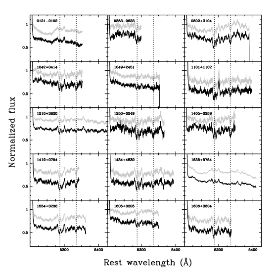
Figure 3.— Central spectra ($\sim$0.54″$\times$1″; normalized to average flux over plotted wavelength region), before (gray) and after (black; shifted arbitrarily by -0.2 for comparison) broad FeII subtraction for the 15 objects for which FeII was subtracted. The location of the stellar absorption lines MgIb $\lambda$5175Å and Fe $\lambda$5270Å is indicated by dotted lines. While some objects show prominent stellar absorption features, for others the region is swamped by AGN emission. Note that the spectra end at the rest wavelength 5600Å/(1+z).

Details of the spectroscopic observations and data reduction are given in Table 2.

4. DERIVED QUANTITIES

In this section, we summarize the results we derive both from the spectral analysis (stellar-velocity dispersion, velocity, and H$\beta$ width) and image analysis (surface photometry and stellar masses) as well as from combining results from both (BH mass and dynamical masses). We will also distinguish between different stellar-velocity dispersion measurements and define the nomenclature we use.

4.1. Spatially-Resolved Stellar-Velocity Dispersion And Velocity

The extracted spatially-resolved Keck spectra allow us to determine the stellar-velocity dispersion as a function of distance from the center. In the following, we will refer to these measurements as $\sigma_{\rm spat}$, in contrast to velocity dispersion determined from aperture spectra, as discussed in the next subsection. The advantage of spatially-resolved spectra is twofold: For one, the spatially-resolved stellar velocity dispersions are not broadened by a rotating disk (if seen edge-on) and second, the contamination by the AGN powerlaw continuum and broad emission lines will only affect the nuclear spectra, but not spectra extracted further out.

A python-based code measures the stellar-velocity dispersion from the extracted spectra, using a linear combination of G&K giant stars taken from the Indo-US survey, broadened to a width ranging between 30-500 km s^-1. In addition, a polynomial continuum of order 3-5 was fitted, depending on the object and fitting region. The code uses a Markov-chain Monte Carlo (MCMC) simulation to find the best-fit velocity dispersion and error; see Suyu et al. (2010) for more detailed description of the fitting technique. Three different regions were fitted: (i) the region around CaT, 8480-8690Å; (ii) the region around MgIb that also includes several Fe absorption lines, 5050-5450Å (i.e. redwards of the [OIII] $\lambda$5006.85Å and the HeI$\lambda\lambda$5015.8,5047.47Å AGN emission lines); and (iii) the region around the CaH+K lines, 3735-4300Å (i.e. bluewards of the broad H$\gamma$ and [OIII] $\lambda$4363.21Å AGN emission lines). In Fig. 4-7, examples of fits are shown for all three regions.

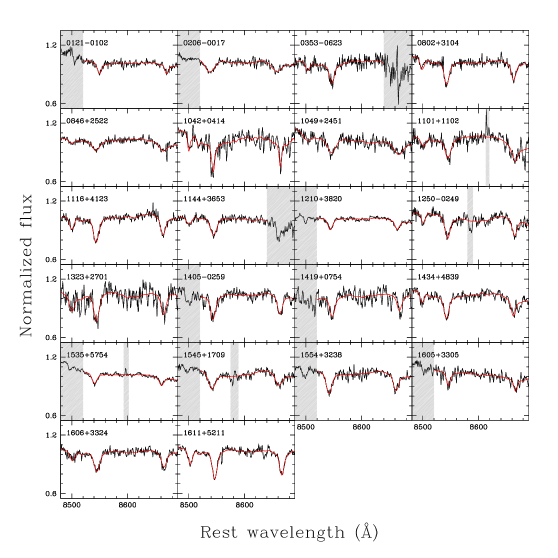
Figure 4.— Examples of stellar-velocity dispersion measurements in CaT region, at a distance of $\sim$0.7″ from the center. The observed spectrum is shown in black, the model in red. The gray-shaded area corresponds to regions that were not included in the fit, due to either AGN emission lines or other spurious artifacts.

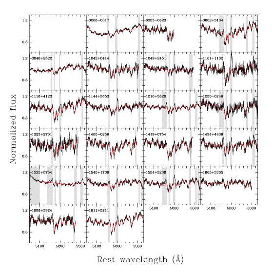
Figure 5.— Same as in Fig. 4, but for the MgIb region. Note that the spectra end at the rest wavelength 5600Å/(1+z). (Object 0121-0102 is not shown here since the S/N is too low to determine $\sigma_{\rm spat}$ from this region.)

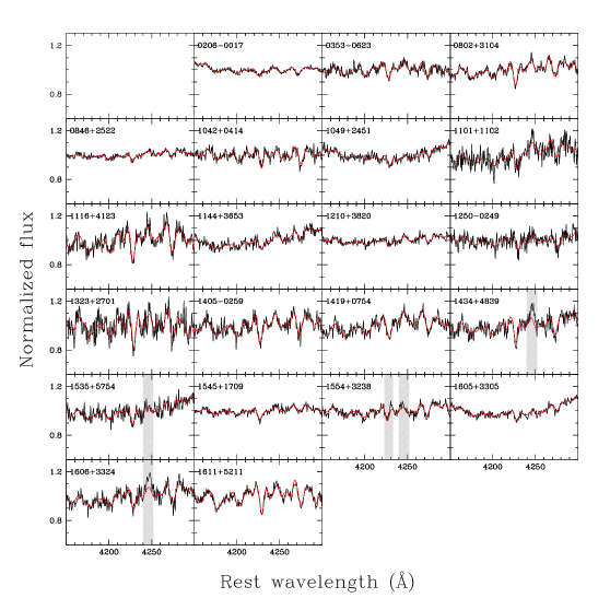
Figure 6.— Same as in Fig. 4, but in a region redwards of CaHK, excluding the CaHK region due to AGN contamination. (Object 0121-0102 is not shown here since the S/N is too low to determine $\sigma_{\rm spat}$ from this region.)

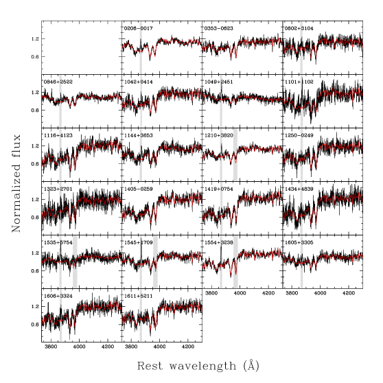
Figure 7.— Same as in Fig. 6 for a region including CaHK at $\sim$1.6″ from the center. (Object 0121-0102 is not shown here since the S/N is too low to determine $\sigma_{\rm spat}$ from this region.)

In region (i), the broad AGN emission line OI $\lambda$8446Å contaminates the spectra in the central region for some objects. In those cases, we excluded the first CaT line and only used the region 8520-8690. In objects at higher redshifts, the third CaT line can be affected by telluric absorption (although we attempted to correct for this effect), and had to be excluded in some cases.

In region (ii), several AGN narrow-emission lines were masked, if present, such as [Fe VI] $\lambda\lambda\lambda$5145.77, 5176.43, 5335.23Å; [Fe VII] $\lambda\lambda$5158.98, 5277.67Å; [NI] $\lambda\lambda$5197.94,5200.41Å; and [CaV] $\lambda$5309.18Å (wavelengths taken from Moore, 1945; Bowen, 1960). The blue spectra end at an observed wavelength of $\sim$5600Å, which corresponds to restframe $\sim$5200Å for our highest redshifted object (z=0.076).

Region (iii) includes AGN emission from e.g., [FeV] $\lambda$4227.49Å and various broad HeI and Balmer lines, that were masked during the fitting procedure. Also, the CaH$\lambda$3969Å line is often filled by AGN emission (H$\epsilon$). Thus, in most cases, we restricted the fitting region to 4150-4300Å for the central spectra (see Fig. 6), due to AGN contamination. Only in the outer parts, the wavelength regime 3735-4300Å was fitted (Fig. 7). In the following, we still generally refer to region (iii) as CaHK region, even though it might not actually include the CaH+K line in the central spectra where it is contaminated by AGN emission.

The code used to determine the stellar-velocity dispersion also gives the line-of-sight velocity. (Note that we set the central velocity to zero.) The resulting measurements for both stellar-velocity dispersion as well as velocity as a function of distance from the center are shown in Figures 8-10.

The error bars are often higher in the center due to AGN contamination. This is also the reason why the error bars for velocity dispersions determined from the MgIb or CaHK region are higher, since in the blue, the contamination by the AGN powerlaw continuum and broad emission lines is more severe than for the CaT region. On the other hand, in the outermost spectra, the S/N is the dominating error source.

For comparison with literature, we choose the velocity dispersion determined from the CaT region as our benchmark, since this is the region least affected by template mismatch (Barth et al., 2002) and AGN contamination from a featureless continuum as well as emission lines (Greene & Ho, 2006b). We calculate the luminosity-weighted line-of-sight velocity dispersion within the spheroid effective radius (determined from the surface photometry of the SDSS DR7 images as outlined below):

$$\sigma_{\rm spat,reff}^{2}=\frac{\int\limits_{\rm-reff}^{\rm reff}\sigma_{\rm spat}^{2}(r)\cdot I(r)\cdot r\cdot dr}{\int\limits_{\rm-reff}^{\rm reff}I(r)\cdot r\cdot dr}$$

with $I(r)$ = $I(\rm{reff})\cdot\exp(-7.67\cdot[(r/r_{\rm reff})^{0.25}-1])$ de Vaucouleurs (1948) profile. (The range “-reff” to “+reff” refers to the fact that we extracted spectra symmetrically around the center of each object, along the major axis, and measured stellar velocity dispersions from each of them; see also Figs. 8-10.) As our $\sigma_{\rm spat}$ measurements are discrete, we interpolate over the appropriate radial range using a spline-function. In the following, we refer to the spatially-resolved stellar-velocity dispersion within the spheroid effective radius as $\sigma_{\rm spat,reff}$. This represents the spheroid-only dispersion within the effective radius, free from broadening due to a rotating disk component. Note that the only place where we show spatially-resolved velocity dispersion at a certain radius is in Figures 8-10 ($\sigma_{\rm spat}$) and in Figure 15a for the ratios; otherwise we always refer to the luminosity-weighted spatially-resolved velocity dispersion within the effective radius $\sigma_{\rm spat,reff}$.

We can in principle choose arbitrary integration limits, to e.g. determine the stellar-velocity dispersion within one-eighth of the effective radius, one-half of the effective radius, or 1.5″ (comparable to SDSS fiber spectra). While these are all “radii” found in the literature, we will not be using them for comparison in this paper, since literature values all refer to aperture data (and not spatially-resolved as discussed here; see next section).

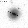
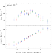
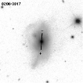
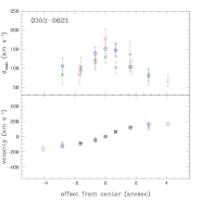
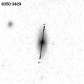
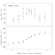
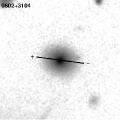
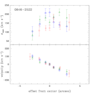
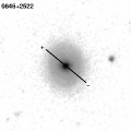
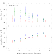
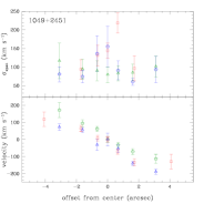
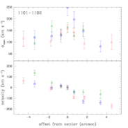
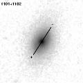
Figure 8.— Spatially-resolved stellar-velocity dispersions and velocities. In the first and third column, we show spatially-resolved stellar-velocity dispersion (upper panel) and velocity curve (lower panel) as derived from CaHK (blue pentagons), MgIb (green triangles), and the CaT region (red squares). In the second and fourth column, the corresponding SDSS-DR7 multi-filter image is shown in gray scales. North is up, east is to the left; same dimensions as in Fig. 1, with the position of the longslit indicated as black line (corresponding to 20″  for clarity, but the slit is 175″ long). The “+” and “-” signs indicate the extraction direction of the spectra, corresponding to the x-axis in the plots. Note that all figures are on the same gray scale to allow for comparison.

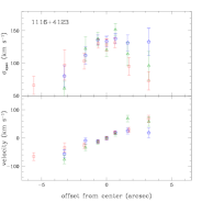
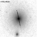
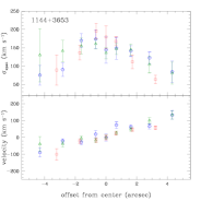
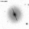
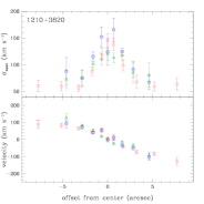
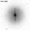
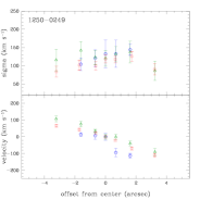
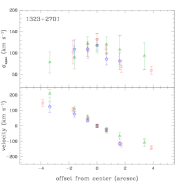
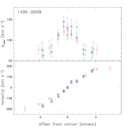
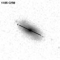
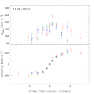
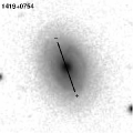
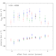
Figure 9.— The same as in Fig. 8.

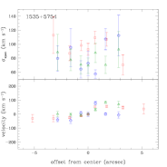
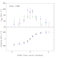
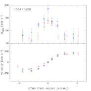
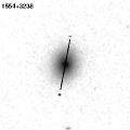
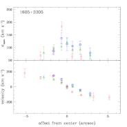
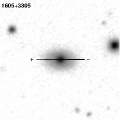
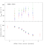
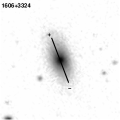
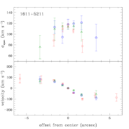
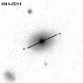
Figure 10.— The same as in Fig. 8.

4.2. Aperture Stellar-Velocity Dispersion

While we consider $\sigma_{\rm spat,reff}$ the spheroid dispersion within the spheroid effective radius free of disk contamination, comparison with literature data (such as fiber-based SDSS data or unresolved aperture spectra for more distant galaxies) requires us to also determine aperture stellar-velocity dispersions. To do so, we extracted 1D spectra by increasing the width of the extraction window by one pixel, leaving the centroid fixed to the central pixel. We then measured the stellar-velocity dispersion for each of the extracted spectra using the same procedure as outlined above. We use the same mask/fitting region as used for the center for the spatially-resolved spectra (since here, all spectra will suffer from the AGN contamination). Also note that broad FeII emission was subtracted for all rows, if present, fixed to the widths determined in the center. We refer to the resulting stellar-velocity dispersion from these spectra as “aperture” $\sigma_{\rm ap}$. Note that $\sigma_{\rm ap}$ not only contains the AGN contamination (continuum and emission lines) independent of extracted aperture (and that is why here the fitting region that we refer to as CaHK region does not actually include the CaH+K line; see § 4.1) but can also be broadened by any rotational component present or biased to lower values in case of contribution of a kinematically cold disk seen face on. Also, the resulting $\sigma_{\rm ap,reff}$ is already luminosity weighted due to the way the spectra are extracted. The results are shown in Fig. 11.

We determine an aperture stellar-velocity dispersion within the effective radius $\sigma_{\rm ap,reff}$ by choosing the aperture size identical to the spheroid effective radius of a given object.

To compare our results with SDSS fiber spectra, we determine $\sigma_{\rm ap,1.5^{\prime\prime}}$, measured from aperture spectra within the central 1.5″ radius as a proxy for what would have been measured with the 3″ diameter Sloan fiber. Note, however, that in fact, our $\sigma_{\rm ap,1.5^{\prime\prime}}$ corresponds to a rectangular region with 1.5″ radius and 1″ width, given the width of the long slit. For eight objects, we can directly compare our results for $\sigma_{\rm ap,1.5^{\prime\prime}}$ with those derived from SDSS fiber spectra by Shen et al. (2008) and Greene & Ho (2006a). While individual objects can differ by up to 25%, slightly larger than the quoted uncertainties for the SDSS spectra ($\sim$10-15%), on average, the measurements agree very well ($\sigma_{\rm ap,1.5^{\prime\prime}}$/$\sigma_{\rm SDSS}$ = 1.05 $\pm$ 0.1).

We summarize the different stellar-velocity dispersion measurements in Table 3, for the CaT region only.

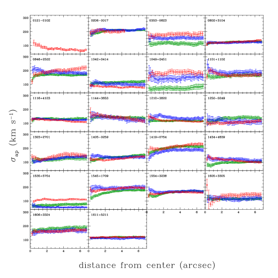
Figure 11.— Stellar-velocity dispersion as derived from the CaHK region (blue pentagons), the MgIb region (green triangles), and the CaT region (red squares). In contrast to Fig. 8-10, the unresolved data is shown here, i.e. using aperture spectra with aperture widths increasing in one pixel steps (corresponding to arcseconds as indicated on the x-axis).

Table 3Stellar-Velocity Dispersion Measurements

Object	$\sigma_{\rm spat,reff}$	$\sigma_{\rm ap,reff}$	$\sigma_{\rm ap,1.5^{\prime\prime}}$	$r_{\rm eff,sph}$
	(km s-1)	(km s-1)	(km s-1)	(kpc)
(1)	(2)	(3)	(4)	(5)
0121-0102	104$\pm$6	89$\pm$10	89$\pm$8	1.54
0206-0017	222$\pm$2	200$\pm$9	213$\pm$8	3.07
0353-0623	159$\pm$6	168$\pm$15	179$\pm$11	1.29
0802+3104	95$\pm$2	128$\pm$5	122$\pm$6	3.17
0846+2522	130$\pm$3	205$\pm$11	190$\pm$11	4.48
1042+0414	60$\pm$1	85$\pm$4	86$\pm$4	2.76
1049+2451	138$\pm$4	189$\pm$15	181$\pm$11	2.78
1101+1102	113$\pm$2	167$\pm$10	178$\pm$9	4.02
1116+4123	104$\pm$2	110$\pm$5	130$\pm$4	3.40
1144+3653	173$\pm$4	154$\pm$12	158$\pm$13	1.26
1210+3820	137$\pm$3	137$\pm$6	124$\pm$5	0.43
1250-0249	112$\pm$2	102$\pm$8	106$\pm$9	2.23
1323+2701	113$\pm$3	119$\pm$8	121$\pm$10	1.53
1405-0259	119$\pm$2	119$\pm$5	117$\pm$5	1.24
1419+0754	181$\pm$2	198$\pm$8	194$\pm$9	2.14
1434+4839	115$\pm$2	118$\pm$5	126$\pm$6	2.16
1535+5754	99$\pm$1	110$\pm$5	114$\pm$5	2.09
1545+1709	157$\pm$2	182$\pm$6	182$\pm$6	1.73
1554+3238	136$\pm$3	152$\pm$5	152$\pm$5	0.66
1605+3305	134$\pm$6	97$\pm$23	115$\pm$12	0.79
1606+3324	130$\pm$3	163$\pm$7	163$\pm$7	1.62
1611+5211	95$\pm$1	122$\pm$3	121$\pm$2	2.41

Note. — Col. (1): Target ID (based on RA and DEC). Col. (2): Spatially-resolved stellar-velocity dispersion within spheroid effective radius from CaT region. Random errors are given, while systematic errors are of order 7-15%. Col. (3): Aperture stellar-velocity dispersion within spheroid effective radius from CaT region. Random errors are given, while systematic errors are of order 7-15%. Col. (4): Aperture stellar-velocity dispersion within 1.5″ (to compare with SDSS fiber data) from CaT region. Random errors are given, while systematic errors are of order 7-15%. Col. (5): Spheroid effective radius (in kpc; semi-major axis) from surface photometry (see Appendix A and Table 5; fiducial error 0.04 dex).

4.3. Black Hole Mass

Black hole masses are estimated using the empirically calibrated photo-ionization method, also sometimes known as “virial method” (e.g., Wandel et al., 1999; Vestergaard, 2002; Woo & Urry, 2002; Vestergaard & Peterson, 2006; McGill et al., 2008). Briefly, the method assumes that the kinematics of the gaseous region in the immediate vicinity of the BH, the BLR, traces the gravitational field of the BH. The width of the broad emission lines (e.g. H$\beta$) gives the velocity scale, while the BLR size is given by the continuum luminosity through application of an empirical relation found from reverberation mapping (RM) (e.g., Wandel et al., 1999; Kaspi et al., 2000, 2005; Bentz et al., 2006). Combining size and velocity gives the BH mass, assuming a dimensionless coefficient of order unity to describe the geometry and kinematics of the BLR (sometimes known as the “virial” coefficient). Generally, this coefficient is obtained by matching the $M_{\rm BH}$-$\sigma$ relation of local active galactic nuclei (AGNs) to that of quiescent galaxies (Onken et al., 2004; Greene & Ho, 2006a; Woo et al., 2010). Alternatively, the coefficient can be postulated under specific assumptions on the geometry and kinematics of the BLR. We adopt the normalizations in McGill et al. (2008), which are consistent with those found by Onken et al. (2004). However, since Woo et al. (2010) find a slightly different f-factor than Onken et al. (2004), causing a decrease in $M_{\rm BH}$ by 0.02 dex, we subtracted 0.02 dex from all BH masses.

4.3.1 H$\beta$ Widths Measurements

To measure the width of the broad H$\beta$ emission, we use the central blue spectrum, extracted with a size of 1.08″$\times$1″. First, underlying broad FeII emission was removed (if needed) as described in § 3. Then, a stellar template was subtracted to correct for stellar absorption lines underlying the broad H$\beta$ line in the following manner: We fixed the stellar-velocity dispersion and velocity to the values determined in the region $\sim$5050-5450Å (i.e. the MgIb region that is mostly free of AGN emission) and then derived a best fitting-model in the region $\sim$4500-5450Å, including a polynomial continuum and outmasking the H$\beta$ and [OIII] $\lambda\lambda$ 4959,5007Å (hereafter [OIII]) emission lines. The resulting stellar-absorption free spectra in the region around H$\beta$ are shown in Fig. 12. Finally, we modeled the spectra by a combination of (i) a linear continuum, (ii) a Gaussian at the location of the narrow H$\beta$ line, (iii) Gauss-Hermite polynomials for both [OIII] lines, with a fixed flux ratio of 1:3 and a fixed wavelength difference, and (iv) Gauss-Hermite polynomials for the broad H$\beta$ line. A truncated Gauss-Hermite series (van der Marel & Franx, 1993; McGill et al., 2008) has the advantage (over symmetrical Gaussians) of taking into account asymmetries in the line profiles that are often present in the case of [OIII] and broad H$\beta$ (Fig. 13). The coefficients of the Hermite polynomials ($h_{3}$, $h_{4}$, etc.) can be derived by straightforward linear minimization; the center and width of the Gaussian are the only two non-linear parameters. For [OIII], we allow coefficients up to $h_{12}$, for H$\beta$ up to $h_{5}$.

From the resulting fit, the second moment of the broad H$\beta$ ($\sigma_{\rm H\beta}$) component is measured within a truncated region that contains only the broad H$\beta$ line as determined interactively for each object (green line in Fig. 13). Note that the line dispersion is defined as follows. The first moment of the line profile is given by

$$\lambda_{0}=\int\lambda P(\lambda)d\lambda/\int P(\lambda)d\lambda$$

and the second moment is

$$\sigma^{2}_{\rm H\beta}=\left<\lambda^{2}\right>-\lambda_{0}^{2}=\left[\int\lambda^{2}P(\lambda)d\lambda/\int P(\lambda)d\lambda\right]-\lambda_{0}^{2}.$$

The square root is the line dispersion $\sigma_{\rm H\beta}$ or root-mean-square (rms) width of the line (see also Peterson et al. 2004).

We estimate the uncertainty in $\sigma_{\rm H\beta}$ taking into account the three main sources of error involved (i) the difference between the fit and the data in the region of the broad H$\beta$ component (to account for uncertainties by asymmetries not fitted by the Gauss-Hermite polynomials); (ii) the systematic error involved when determining the size of the fitting region (which we determined empirically to be of the order of 5%), and (iii) the statistical error determined by repeated fitting using the same fitting parameters (of order 1%). Note that due to the very high S/N, the line dispersion inferred from the Gauss-Hermite polynomial fit is virtually indistinguishable from that measured directly from the data (on average, fit/data=1$\pm$0.02 and at most, the difference is 5%). We also compare $\sigma_{\rm H\beta}$ with that inferred from the FHWM assuming a Gaussian profile: $\sigma_{\rm H\beta}$/(FHWM/2.355) = 1.11$\pm$0.3. The average difference of 10%, expected because broad lines are known not to be Gaussian in shape, corresponds to a systematic difference of 0.04 dex, negligible for an individual object, and small compared to the uncertainty on the BH mass that we assume (0.4 dex), but potentially a significant source of bias for accurate measurements based on large samples.

Fig. 13 shows the fit for all objects. The variety of broad H$\beta$ profiles is interesting, with only 6/25 objects revealing symmetric line profiles, 8/25 objects having more than one peak, and the majority of objects (11/25) having asymmetric line profiles, thus showing the need for Gauss-Hermite polynomials. While the line profile can in principle provide insights into BLR geometry and kinematics, this is beyond the scope of the present paper. Note that the narrow H$\beta$/[OIII] $\lambda$5007Å ratio ranges between 6-28%, in agreement with other studies (e.g., Marziani et al., 2003; Woo et al., 2006).

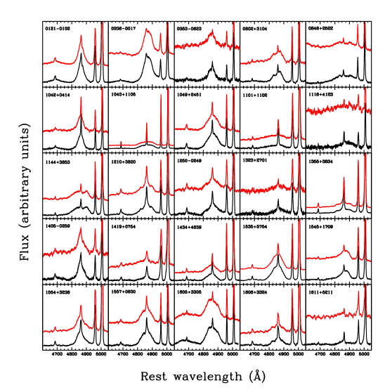
Figure 12.— Spectra around the broad H$\beta$ emission before (upper spectra; red) and after subtraction of stellar absorption and continuum (lower spectra; black).

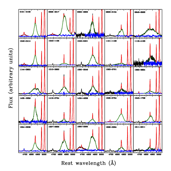
Figure 13.— Determination of the second moment of the broad H$\beta$ emission. In addition to a continuum, the narrow H$\beta$ component was fitted by a Gaussian while the broad H$\beta$ and both [OIII] lines were fitted by Gaussian-Hermite polynomials (see text for details). In some cases, strong broad and narrow HeII emission overlaps with the broad H$\beta$ component and was fitted additionally with a broad and narrow Gaussian. The observed spectrum is shown in black, the total fit in red and the residual in blue (only in the region that was fitted). The region of the fit in which the second moment of the broad H$\beta$ component was determined is shown as green line. Note the variety of H$\beta$ profiles. For 1535+5754, prominent [FeIII] $\lambda$4658Å and [ArIV] $\lambda\lambda$4711,4740Å emission is present in the spectrum and each of these emission lines was fitted by a Gaussian component.

4.3.2 Luminosity at 5100Å and BH masses

We use the SDSS images to simultaneously fit the AGN by a point-spread function (PSF) and the host galaxy by spheroid and disk (if present). The next section and Appendix A describe the surface photometry in detail. The resulting PSF g’-band magnitude is corrected for Galactic extinction (subtracting the SDSS DR7 “extinction_g”’ column), and then extrapolated to 5100Å, assuming a powerlaw of the form $f_{\nu}\propto\nu^{\alpha}$ with $\alpha$=-0.5. (Literature values of $\alpha$ range between -0.2 and -1; Malkan et al. 1983; Neugebauer et al. 1987; Cristiani & Vio 1990; Francis et al. 1991; Zheng et al. 1997; Vanden Berk et al. 2001; see also Bennert et al. 2010 and D. Szathmáry et al. 2011, submitted).

We calculated BH masses according to the following formula (McGill et al., 2008):

$$\log M_{\rm BH}=7.68+2\log\left(\frac{\sigma_{\rm H_{\beta}}}{1000\,{\rm km\,s^{-1}}}\right)+0.518\log\left(\frac{\lambda L_{5100}}{10^{44}\,{\rm erg\,s^{-1}}}\right)$$

The results are given in Table 4.

We assume a nominal uncertainty of the BH masses measured via the virial method of 0.4 dex. Note that we do not correct for possible effects of radiation pressure (e.g., Marconi et al., 2008, 2009, see, however, Netzer 2009, 2010).

Table 4BH Mass Measurements

Object	$\sigma_{\rm H\beta}$	$\lambda$$L_{\rm 5100}$	log $M_{\rm BH}/M_{\sun}$
	(km s-1)	(1044 erg s-1)
(1)	(2)	(3)	(4)
0121-0102	1317$\pm$66	0.24	7.58
0206-0017	1991$\pm$100	0.61	8.15
0353-0623	1694$\pm$85	0.09	7.58
0802+3104	1472$\pm$74	0.05	7.31
0846+2522	4547$\pm$227	0.24	8.66
1042+0414	1252$\pm$63	0.04	7.12
1043+1105	1910$\pm$96	0.16	7.81
1049+2451	2252$\pm$113	0.18	7.98
1101+1102	2900$\pm$145	0.05	7.91
1116+4123	2105$\pm$105	0.03	7.51
1144+3653	2551$\pm$128	0.01	7.50
1210+3820	2377$\pm$119	0.03	7.64
1250-0249	2378$\pm$119	0.06	7.79
1323+2701	2133$\pm$107	0.02	7.12
1355+3834	3110$\pm$156	0.09	8.10
1405-0259	1343$\pm$67	0.05	7.22
1419+0754	1932$\pm$97	0.08	7.65
1434+4839	1572$\pm$79	0.14	7.62
1535+5754	2019$\pm$101	0.26	7.97
1545+1709	1604$\pm$80	0.06	7.42
1554+3238	1988$\pm$99	0.11	7.77
1557+0830	2019$\pm$101	0.08	7.69
1605+3305	1981$\pm$99	0.23	7.92
1606+3324	1737$\pm$87	0.03	7.36
1611+5211	1843$\pm$92	0.04	7.49

Note. — Col. (1): Target ID (based on RA and DEC). Col. (2): Second moment of broad H$\beta$. Col. (3): Rest-frame luminosity at 5100Å determined from SDSS g’ band surface photometry (fiducial error 0.1 dex). Col. (4): Logarithm of BH mass (solar units) (uncertainty of 0.4 dex).

4.4. Surface Photometry

To obtain a host-galaxy free 5100Å luminosity (for an accurate BH mass measurement) as well as a good estimate of the spheroid effective radius (to measure the stellar-velocity dispersion at the effective radius), we performed surface photometry of archival SDSS DR7 images. In our previous papers, we ran the 2D galaxy fitting program GALFIT (Peng et al., 2002) on high-spatial resolution HST images for this purpose. Here, we lack space-based images, but - compared to our previous studies - the objects are at much lower redshifts ($z$$\simeq$0.05 compared to $z$$\simeq$0.4 and 0.6). (Note that the average seeing ranges between $\sim$1.2″ in the z’-band to $\sim$1.4″ in the g’-band for our sample.) Moreover, the SDSS images come in five different filters (u’,g’,r’,i’,z’), allowing us to determine the host-galaxy properties by simultaneously fitting the multiple bands while imposing certain constraints between the parameters of each band. Since this is beyond the scope of GALFIT, we developed a new image analysis code. The advantage of a joint multi-band analysis is that it enables us to more easily distinguish between the AGN which dominates in the blue bands from the host galaxy which is dominant in the redder filters. The code is described in detail in Appendix A, including a comparison with GALFIT. The results are summarized in Table 5.

Note that as a sanity check, we checked the classic galaxy scaling relations (see e.g., Hyde & Bernardi, 2009a, b), such as fundamental plane (FP) or stellar mass vs $\sigma_{\rm ap,reff}$ and stellar mass vs $r_{\rm eff,sph}$. Taking into account the small dynamic range and sample size (especially when considering elliptical host galaxies only), the results are consistent within the errors. We will show and discuss these galaxy scaling relations when presenting the full sample in the upcoming papers of this series.

Table 5Results from Surface Photometry

Object	PSF				Spheroid				Disk				$\log L_{\rm sph,V}/L_{\odot}$	$r_{\rm eff,sph}$
	g’	r’	i’	z’	g’	r’	i’	z’	g’	r’	i’	z’
	(mag)	(mag)	(mag)	(mag)	(mag)	(mag)	(mag)	(mag)	(mag)	(mag)	(mag)	(mag)		(kpc)
(1)	(2)	(3)	(4)	(5)	(6)	(7)	(8)	(9)	(10)	(11)	(12)	(13)	(14)	(15)
0121-0102	17.01	17.51	17.07	17.24	16.39	16.15	15.77	15.56	15.52	14.93	14.64	14.52	10.19$\pm$0.07	1.54
0206-0017	15.47	15.75	15.65	15.72	14.68	13.98	13.59	13.32	15.39	14.63	14.23	14.00	10.80$\pm$0.07	3.07
0353-0623	18.80	18.99	18.52	18.64	17.53	16.72	16.38	16.17	18.03	17.32	16.95	16.74	10.20$\pm$-0.06	1.29
0802+3104	18.13	18.28	17.77	17.67	15.76	15.13	14.79	14.57	$\cdots$	$\cdots$	$\cdots$	$\cdots$	10.30$\pm$0.06	3.17
0846+2522	16.86	16.85	16.67	16.61	16.01	15.37	15.00	14.78	$\cdots$	$\cdots$	$\cdots$	$\cdots$	10.03$\pm$-0.06	4.48
1042+0414	18.94	19.26	18.80	18.97	16.82	16.09	15.63	15.36	$\cdots$	$\cdots$	$\cdots$	$\cdots$	10.15$\pm$0.06	2.76
1043+1105	17.14	17.37	16.91	17.08	16.87	16.50	16.14	16.10	$\cdots$	$\cdots$	$\cdots$	$\cdots$	9.90$\pm$0.06	3.55
1049+2451	17.36	17.56	17.09	17.12	16.45	15.83	15.40	15.19	$\cdots$	$\cdots$	$\cdots$	$\cdots$	10.30$\pm$0.06	2.78
1101+1102	17.77	17.51	17.32	17.31	16.43	15.35	15.07	14.71	16.74	16.19	15.73	15.50	10.04$\pm$0.20	4.02
1116+4123	56.05	18.96	18.80	17.88	14.97	14.21	13.85	13.63	$\cdots$	$\cdots$	$\cdots$	$\cdots$	10.13$\pm$0.40	3.40
1144+3653	19.36	21.32	22.10	52.97	16.47	15.59	15.19	14.90	16.12	15.39	15.10	14.88	10.03$\pm$0.10	1.26
1210+3820	17.28	16.70	17.21	16.91	15.81	15.13	14.74	14.45	15.28	14.55	14.21	13.97	9.84$\pm$0.36	0.43
1250-0249	18.15	18.23	17.89	17.77	17.53	16.54	16.08	15.79	15.97	15.29	14.91	14.64	9.84$\pm$0.06	2.23
1323+2701	19.60	19.12	18.74	18.28	19.07	18.25	17.62	17.43	17.93	17.14	16.78	16.49	9.36$\pm$0.06	1.53
1355+3834	17.93	17.92	17.21	17.58	16.55	16.15	15.73	15.60	$\cdots$	$\cdots$	$\cdots$	$\cdots$	10.11$\pm$0.06	2.06
1405-0259	18.79	19.02	18.49	18.62	17.72	16.82	16.54	16.19	16.68	15.92	15.53	15.21	9.84$\pm$0.06	1.24
1419+0754	18.32	18.18	17.48	17.49	16.85	15.71	15.21	14.84	15.51	14.86	14.49	14.29	10.32$\pm$0.06	2.14
1434+4839	16.67	16.73	16.61	16.61	15.83	15.15	14.81	14.57	16.10	15.47	15.16	14.94	10.18$\pm$0.11	2.16
1535+5754	15.61	15.61	15.67	15.62	15.34	14.76	14.44	14.30	$\cdots$	$\cdots$	$\cdots$	$\cdots$	10.20$\pm$0.24	2.09
1545+1709	18.33	18.08	17.69	17.35	17.41	16.77	16.31	16.15	17.69	16.90	16.50	16.17	9.80$\pm$0.06	1.73
1554+3238	17.57	17.58	17.30	17.15	17.60	16.73	16.30	16.12	16.38	15.71	15.37	15.09	9.79$\pm$0.06	0.66
1557+0830	17.92	17.92	17.59	17.51	17.18	16.64	16.30	16.16	$\cdots$	$\cdots$	$\cdots$	$\cdots$	9.81$\pm$0.06	1.18
1605+3305	17.03	16.42	16.20	16.07	17.08	16.40	16.19	16.20	$\cdots$	$\cdots$	$\cdots$	$\cdots$	9.98$\pm$0.06	0.79
1606+3324	19.37	19.77	18.72	19.14	17.46	16.54	16.10	15.78	17.61	16.85	16.45	16.27	10.05$\pm$0.06	1.62
1611+5211	18.23	17.74	17.47	17.18	16.15	15.43	15.03	14.80	$\cdots$	$\cdots$	$\cdots$	$\cdots$	10.18$\pm$0.06	2.41

Note. — Col. (1): Target ID (based on RA and DEC). Col. (2-5): Extinction-corrected g’, r’, i’, and z’ PSF magnitudes (with an uncertainty of 0.5 mag). Col. (6-9): Extinction-corrected g’, r’, i’, and z’ spheroid magnitudes (with an uncertainty of 0.2 mag). Col. (10-13): Extinction-corrected g’, r’, i’, and z’ disk magnitudes (with an uncertainty of 0.2 mag). Col. (14): Logarithm of spheroid luminosity in rest-frame V (solar units). Col. (15): Spheroid effective radius (in kpc; semi-major axis).

4.5. Stellar and Dynamical Spheroid Mass

Our surface photometry code gives spheroid, disk, and total host-galaxy magnitudes for four different SDSS filters (g’, r’, i’, z’) which can in turn be used to estimate stellar spheroid masses. For this purpose, Auger et al. (2009) have developed a Bayesian stellar mass estimation code that we use here. The code allows informative priors to be placed on the age, metallicity, and dust content of the galaxy and uses a MCMC sampler to explore the full parameter space and quantify degeneracies between the stellar population parameters. We use a Chabrier initial-mass function (IMF).

Also, with the knowledge of $\sigma_{\rm ap,reff}$ (as determined from the CaT region) and $r_{\rm eff,sph}$, we can calculate a dynamical mass:

$$M_{\rm sph,dyn}=kr_{\rm eff,sph}\sigma_{\rm ap,reff}^{2}/G$$

with $G$ = gravitational constant. For comparison with literature (in particular Marconi & Hunt, 2003), we use $k=3$. For the same reason, we choose $\sigma_{\rm ap,reff}$ instead of $\sigma_{\rm spat,reff}$. The results are given in Table 6.

Table 6Dynamical And Stellar Masses

Object	$\log M_{\rm sph,vir}/M_{\odot}$	$\log M_{\rm sph,\star}/M_{\odot}$	$\log M_{\rm disk,\star}/M_{\odot}$	$\log M_{\rm host,\star}/M_{\odot}$
(1)	(2)	(3)	(4)	(5)
0121-0102	9.866	10.12$\pm$0.24	10.60$\pm$0.24	10.75$\pm$0.23
0206-0017	10.93	10.95$\pm$0.23	10.71$\pm$0.22	11.17$\pm$0.23
0353-0623	10.41	10.33$\pm$0.22	10.08$\pm$0.23	10.52$\pm$0.22
0802+3104	10.56	10.38$\pm$0.23	$\cdots$	$\cdots$
0846+2522	11.12	10.50$\pm$0.23	$\cdots$	$\cdots$
1042+0414	10.15	10.32$\pm$0.23	$\cdots$	$\cdots$
1043+1105a	$\cdots$	9.83$\pm$0.24	$\cdots$	$\cdots$
1049+2451	10.84	10.41$\pm$0.23	$\cdots$	$\cdots$
1101+1102	10.89	10.33$\pm$0.22	9.89$\pm$0.23	10.46$\pm$0.22
1116+4123	10.46	10.20$\pm$0.22	$\cdots$	$\cdots$
1144+3653	10.32	10.26$\pm$0.22	10.21$\pm$0.24	10.54$\pm$0.23
1210+3820	9.753	9.94$\pm$0.24	10.13$\pm$0.24	10.35$\pm$0.23
1250-0249	10.21	10.14$\pm$0.22	10.50$\pm$0.22	10.65$\pm$0.22
1323+2701	10.30	9.65$\pm$0.22	9.93$\pm$0.23	10.10$\pm$0.23
1355+3834a	$\cdots$	10.11$\pm$0.23	$\cdots$	$\cdots$
1405-0259	10.09	10.04$\pm$0.23	10.42$\pm$0.22	10.58$\pm$0.22
1419+0754	10.77	10.73$\pm$0.21	10.78$\pm$0.24	11.00$\pm$0.24
1434+4839	10.33	10.30$\pm$0.24	10.13$\pm$0.24	10.53$\pm$0.23
1535+5754	10.19	10.24$\pm$0.24	$\cdots$	$\cdots$
1545+1709	10.6	9.92$\pm$0.22	9.93$\pm$0.22	10.23$\pm$0.22
1554+3238	10.03	10.00$\pm$0.23	10.32$\pm$0.23	10.50$\pm$0.23
1557+0830a	$\cdots$	9.82$\pm$0.23	$\cdots$	$\cdots$
1605+3305	9.712	9.95$\pm$0.23	$\cdots$	$\cdots$
1606+3324	10.48	10.33$\pm$0.22	10.06$\pm$0.24	10.50$\pm$0.23
1611+5211	10.4	10.33$\pm$0.22	$\cdots$	$\cdots$

Note. — Col. (1): Target ID (based on RA and DEC). Col. (2): Dynamical spheroid mass calculated from $r_{\rm eff,sph}$ and $\sigma_{\rm ap,reff}$ (determined from CaT region; fiducial error 0.1 dex). Col. (3): Stellar spheroid mass (using Chabrier as IMF). Col. (4): Stellar disk mass (if present). Col. (5): Stellar host mass (only listed if disk present, i.e. if different from (3)). ^a: For three objects, dynamical masses could not be determined as $\sigma_{\rm ap,reff}$ could not be reliably measured.

5. COMPARISON SAMPLES

For the $M_{\rm BH}$-scaling relations, we compile comparison samples from the literature, including local inactive galaxies (Marconi & Hunt, 2003; Häring & Rix, 2004; Gültekin et al., 2009) and local active galaxies (Greene & Ho, 2006a; Woo et al., 2010). Note that while for the inactive galaxies, BH masses have been derived from direct dynamical measurements, the BH masses for active galaxies are calibrated masses either from reverberation mapping or from the virial method.

5.1. $M_{\rm BH}$-$\sigma$ Relation

For the $M_{\rm BH}$-$\sigma$ relation, we use the data from Gültekin et al. (2009) (local inactive galaxies), Greene & Ho (2006a) (local active galaxies), and Woo et al. (2010) (local RM AGNs). In all cases, the stellar-velocity dispersion measurements correspond to luminosity-weighted stellar-velocity dispersions within a given aperture $\sigma_{\rm ap}$. For Gültekin et al. (2009), the aperture is typically the effective radius, but as $\sigma_{\rm ap}$ is compiled from the literature, there are also cases where it is $\sigma_{\rm ap,1/8reff}$ or $\sigma_{\rm c}$. However, Gültekin et al. (2009) conclude that the systematic differences are small compared to other systematic errors. The BH masses were determined from direct dynamical measurements (stellar or gaseous kinematics or masers). In total, data are available for 49 objects with $z<0.04$. For Greene & Ho (2006a), $\sigma_{\rm ap,1.5^{\prime\prime}}$ was determined from the fiber-based SDSS spectra and is thus within an aperture of 1.5″ radius. From their sample of 56 Seyfert-1 galaxies with $z<0.1$, Woo et al. (2008) chose a sub-sample of 49 objects for which they measured BH mass using the line dispersion of H$\beta$ and the H$\alpha$ luminosity consistently calibrated to our BH mass measurements (McGill et al., 2008). These 49 objects have 5 objects in common with our sample, so we use our results instead, leaving us with 44 local SDSS AGNs. (We will perform a comparison for the objects in common to both samples once we have our full sample available for which we expect to have a total of $\sim$20 objects in common.) Finally, we include 24 local Seyfert-1 galaxies ($z<$0.09) for which the BH mass has been determined via RM (Woo et al., 2010). For these objects, the $\sigma_{\rm ap}$ measurements were measured within an aperture of typically $\sim$1″$\times$1.5″ to $\sim$1.5″$\times$3″.

To compare our results with these literature data which all consist of luminosity-weighted stellar-velocity dispersions within some aperture, we use $\sigma_{\rm ap,1.5^{\prime\prime}}$ as determined from the CaT region (which is considered the benchmark). (Note that choosing $r_{\rm eff}$ instead as aperture size does not change the results within the errors; see Table 3.)

5.2. $M_{\rm BH}$-$L_{\rm sph}$ and $M_{\rm BH}$-$M_{\rm sph}$ Relations

For the $M_{\rm BH}$-$L_{\rm sph}$ relation, we again use the local inactive sample from Gültekin et al. (2009), here limited to 35 elliptical and S0 galaxies with a reliable spheroid-disk decomposition.

For the $M_{\rm BH}$-$M_{\rm sph,\star}$ relation, we use the J, H, and K magnitudes from Marconi & Hunt (2003) for their group 1 (i.e. with secure BH masses and reliable spheroid luminosities) to calculate stellar masses in the same way we calculated our stellar masses. Also, we updated the BH masses using those listed in Gültekin et al. (2009). This leaves us with a sample of 18 objects.

Finally, for the $M_{\rm BH}$-$M_{\rm sph,dyn}$ relation, we compile local inactive galaxies using BH masses from Gültekin et al. (2009), and calculate dynamical masses using $r_{\rm reff,sph}$ given by Marconi & Hunt (2003) and $\sigma_{\rm ap}$ measurements by Gültekin et al. (2009).

6. RESULTS AND DISCUSSION

Here, we describe and discuss our results. After a brief section on host-galaxy morphologies, merger rates and rotation curves, we focus on the different methods to derive stellar-velocity dispersions and perform a quantitative comparison. Finally, we present the different BH mass scaling relations and compare our results to literature data. Since the aim of this paper is to outline the methodology and present the results of our pilot study, we postpone any detailed quantitative conclusions to the upcoming papers, once the full sample is available.

6.1. Host-Galaxy Morphologies, Merger Rates, And Rotation Curves

Using the multi-filter SDSS images shown in Fig. 1, we can determine the overall host-galaxy morphologies. Given the low spatial resolutions, we divide the sample into three categories: ellipticals (E), S0/a, and spirals later than Sa (S). 11/25 objects can then be classified as S, 9/25 as E, and 5/25 as S0/a. One object with a spiral-like host galaxy morphology is clearly undergoing a merger (0206-0017). 1419+0754 shows irregular structure differing from normal spiral arms and might also be in the process of merging.

The fraction of ellipticals (36$\pm$11%) is somewhat higher than expected, given that these are (almost all radio-quiet) Seyfert galaxies for which the majority has typically been found to reside in spirals or S0 ($\sim$80%, e.g. Hunt & Malkan 1999 and references therein). However, due to the low-resolution ground-based imaging data, and the small number statistics, there is still some uncertainty in this classification, with some objects potentially falling in the neighboring category. Also, we cannot exclude that in a few cases, the images are too shallow to reveal the presence of the disk. Indeed, the majority of objects ($\sim$13/22) show rotation curves with a maximum velocity between 100 and 200 km s^-1. Also the object with a clear merger signature (0206-0017) shows a prominent rotation curve with a maximum of 200 km s^-1 rotational velocity, hinting at a spiral galaxy experiencing a merger event. Both, the variety of host-galaxy morphologies, in particular with a substantial fraction of host galaxies having prominent spiral arms and disk, Hubble types Sa and later (44$\pm$5%), and the rotation curves underscore that their kinematic structure is complex and indeed spatially-resolved information is necessary.

The merger rate (0.06$\pm$0.02) is lower than for our higher redshift objects (0.29$\pm$0.1 at $z\simeq 0.4$; Bennert et al., 2010) and more comparable to inactive galaxies in the local Universe (e.g., Patton et al., 2002, see, however, Tal et al. 2009). The merger rate is likely to be a function of galaxy mass, with higher (major) merger rates for higher mass objects (e.g., Hopkins et al., 2010). Indeed, the local sample studied here has, on average, lower host-galaxy luminosities (25 objects; $\log L_{\rm host;L_{\odot}}$ = 10.33$\pm$0.05; rms scatter: 0.29) than the one at $z\simeq 0.4$ (34 objects; $\log L_{\rm host;L_{\odot}}$ = 10.54$\pm$0.03; rms scatter: 0.18; Bennert et al. (2010)), indicating lower mass objects. However, we suffer from low number statistics and will get back to this discussion, once we have analyzed our full sample of $\sim$100 local Seyfert-1 galaxies.

Note that the image quality does not allow us to determine the fraction of bars present in the host galaxies to study the effect of bars on the $M_{\rm BH}$-$\sigma$ scaling relation (e.g., Graham et al., 2010, and references therein).

6.2. Stellar-Velocity Dispersions

We here compare the various stellar-velocity dispersions; first spatially-resolved vs aperture stellar-velocity dispersions, then the results from three different spectral regions.

6.2.1 Spatially-resolved vs. aperture stellar-velocity dispersions

Figs. 8-10 show the spatially-resolved velocity dispersions for the sample. We are tracing the velocity dispersion for the central 2-6″ radius, depending on the object. For the majority of objects ($\sim$17/22), the overall behavior of $\sigma_{\rm spat,CaT}$ can be described as decreasing from a central value of $\sim$130-200 km s^-1 to a value of $\sim$50-100 km s^-1 in the outer parts. For the remaining objects (5/22), $\sigma_{\rm spat,CaT}$ is roughly constant with radius, within the errors.

A different picture emerges when looking at the aperture stellar-velocity dispersions in Fig. 11. Here, categorizing the overall behavior of $\sigma_{\rm ap,CaT}$ as a function of “radius” (which is here the increase in width of the aperture spectrum), splits the sample into three categories, with the majority of objects (9/22) showing a constant $\sigma_{\rm ap,CaT}$, and the rest distributes with roughly even numbers on either decreasing (6/22) or increasing (7/22) $\sigma_{\rm ap,CaT}$ with radius. Looking at individual objects, 6 objects have a decreasing $\sigma_{\rm ap,CaT}$ with radius in the spatially-resolved spectra but shift towards an apparently increasing $\sigma_{\rm ap,CaT}$ in the aperture spectra due to the rotational support (as reflected in the rotation curve). However, overall, the aperture dispersions change only slowly with radius, as has already been noted by Capellari et al. (1996) and Gebhardt et al. (2000) for inactive galaxies.

We can make a more direct comparison between $\sigma_{\rm spat,reff}$ determined from the spatially-resolved spectra with that determined from the aperture spectra $\sigma_{\rm ap,reff}$, choosing the stellar-velocity dispersion determined from the CaT region (see also Table 3). We divide the sample into three sub-categories according to the host-galaxy morphology (Elliptical, S0/a, Spiral) and additionally distinguish between host galaxies seen face-on and edge-on. Fig. 14 shows the result both as function of effective radius and $\sigma_{\rm spat,reff}$. The general trend conforms to our expectations: If a spiral galaxy is seen edge-on, the rotation component can bias $\sigma_{\rm ap,reff}$ towards higher values and thus, “triangles” are expected to lie below the unity line. However, since the disk is kinematically cold, it can also result in the opposite effect, i.e. biassing $\sigma_{\rm ap,reff}$ towards smaller values, if the disk is seen face on, so “circles” are expected to lie above the unity line. On average, face-on spiral host galaxies objects have $\sigma_{\rm spat,reff}$/$\sigma_{\rm reff,ap}$ = 1.02$\pm$0.05 (rms scatter: 0.24) and edge-on objects have $\sigma_{\rm spat,reff}$/$\sigma_{\rm reff,ap}$ = 0.90$\pm$0.03 (rms scatter: 0.16). If we calculate the average for the whole sample (all morphologies and orientations), $\sigma_{\rm spat,reff}$/$\sigma_{\rm ap,reff}$ = 0.93$\pm$0.04 (rms scatter: 0.2). There is no obvious trend with either bulge mass, BH mass, or effective radius.

To compare the stellar-velocity dispersion measurements with what would be measured from SDSS fiber spectra, we use $\sigma_{\rm ap,1.5^{\prime\prime}}$. For $\sigma_{\rm spat,reff}$/$\sigma_{\rm ap,1.5^{\prime\prime}}$, the same trend persists as for $\sigma_{\rm spat,reff}$/$\sigma_{\rm ap,reff}$, showing that choosing 1.5″ instead of effective radius does not have a large effect on the resulting stellar-velocity dispersion. This can be attributed both to the luminosity weighting with a steep central surface-brightness profile (de Vaucouleurs, 1948) and to the fact that the average effective radius of our sample is close to 1.5″ (2.6$\pm$0.07″; rms scatter: 1.8).

For objects at higher redshift, the effect can be more pronounced as different sizes are involved. Considering our $z$$\sim$0.4 Seyfert-1 sample for which we study the evolution of the $M_{\rm BH}$-scaling relations (Treu et al., 2004; Woo et al., 2006; Treu et al., 2007; Woo et al., 2008; Bennert et al., 2010), the typical extraction window to determine $\sigma_{\rm ap}$ is 1 square-arcseconds, with 1″ corresponding to 5 kpc at that redshift (Woo et al., 2008, J.-H. Woo et al. 2011, in preparation). This is a factor of $\sim$2.8 larger than the actual effective radius determined from surface-brightness photometry for these objects (Bennert et al., 2010, excluding objects with only upper limits of the spheroid radius). If we make another comparison, $\sigma_{\rm spat,reff}$/$\sigma_{\rm ap,2.8\cdot reff}$ = 0.91$\pm$0.05 (rms scatter: 0.2): On average, aperture spectra can overestimate the spheroid-only stellar-velocity dispersion by 0.03$\pm$0.02 dex. This is attributable to a rotational broadening in edge-on objects. Note that the fraction of spiral host galaxies in the sample at $z$$\sim$0.4 ($\sim$14/34) is comparable to the fraction in the local sample studied here ($\sim$9/25) and thus, such a comparison is straightforward.

However, the bias introduced by measuring stellar-velocity dispersions from aperture spectra, even with extraction windows much larger than the effective radius, cannot explain the observed offset of $z$$\sim$0.4 Seyfert-1 galaxies from the $M_{\rm BH}$-$M_{\rm sph}$ scaling relation seen in Woo et al. (2008): For a given BH mass, $\sigma_{\rm ap}$ is too low for the high-z Seyfert galaxies - the opposite effect to the average bias determined here. $\sigma_{\rm ap}$ can be underestimated in case of face-on spiral galaxies with a contribution of the dynamically cold disk, but this effect is too small (on average less than 0.01 dex when considering face-on spirals only; see above). We performed the same comparisons also for the other spectral fitting regions (since the region around MgIb was used in Woo et al. 2008), finding similar results. To conclude, aperture effects can introduce a small bias in the $\sigma$ measurements but cannot explain the offset seen in the $M_{\rm BH}$-$\sigma$ relation for higher-redshift objects (Woo et al., 2008).

Another more recent study that benefits from our comparison between stellar-velocity dispersions derived from aperture spectra to those derived from spatially-resolved spectra is the one by Greene et al. (2010): They report that a sample of water megamaser residing in spiral galaxies in the local Universe ($\sim 0.01<z<0.03$) for which BH masses were derived directly from the dynamics of the H₂O masers fall below the $M_{\rm BH}$-$\sigma$ relation defined by inactive elliptical galaxies. As pointed out by the authors, given the nature of the host galaxies of these megamasers - early-to-mid-type spirals - a bias of the stellar velocity dispersion measurements from aperture spectra due to the presence of the disk is expected. In principle, a rotational component could bias the stellar-velocity dispersion measurements to higher values and result in the observed offset. However, out of their eight objects, only three are significant outliers (their Figs. 8 and 9), namely NGC 2273, NGC 6323, and NGC 2960. Two of these are seen close to face-on (NGC 2273 and NGC 2960; their Fig. 6 and 7) in which case the effect of the disk component on the stellar-velocity dispersion measured from aperture spectra cannot explain the observed offset. Only for NGC 6323, for which the disk is seen close to edge-on (their Fig. 6) could the observed offset indeed be due to rotational broadening. From our Fig. 14, we estimate that the stellar velocity dispersion measured from aperture spectra can overestimate that from spatially resolved measurements by up to $\sim$40% in case of rotational broadening by a disk component seen edge on - large enough to move NGC 6323 close to the local relation defined by ellipticals. To conclude, while for individual objects, the effect of a disk on the derived stellar-velocity dispersion from aperture spectra can be significant, it cannot explain the offset observed by Greene et al. (2010) for their full sample of megamasers.

Figure 14.— Comparison between different stellar-velocity dispersion measurements, in all cases determined from the CaT region. Ratio between $\sigma_{\rm spat,reff}$, i.e. luminosity-weighted stellar-velocity dispersion within effective radius as determined from spatially-resolved spectra and $\sigma_{\rm ap,reff}$ as determined from spectra extracted with an aperture equal to the effective radius, as function of effective radius. The upper panel shows all objects for which the host galaxy has been classified as ellipticals, the middle panel objects with S0/a-type host-galaxy morphology, and the lower panel objects hosted by spirals. The triangles (circles) correspond to galaxies seen edge-on (face-on). The error bars are omitted for clarity, measurement errors on the ratios range between 5-10%.

6.2.2 Stellar-velocity dispersions from different spectral regions

When comparing stellar-velocity dispersion measurements from the three different spectral regions, the overall picture is that they agree within the errors. A more quantitative comparison is shown in Fig. 15. For the aperture data, three extreme outliers were excluded in this figure due to contaminating broad AGN emission lines and featureless continuum swamping the blue spectral region (namely 0353-0623, 1049+2451, 1535+5754; see also Fig. 11). These outliers are shown in the one-to-one plot of $\sigma_{\rm CaT}$ vs. $\sigma_{\rm MgIb}$ and $\sigma_{\rm CaHK}$ within the effective radii as open symbols (Fig. 15b). (Note that none of the objects was excluded for the spatially-resolved data, explaining the higher scatter.)

In general, for the spatially-resolved stellar-velocity dispersions (Fig. 15a, left panels) both ratios $\sigma_{\rm spat,CaT}$/$\sigma_{\rm spat,MgIb}$ and $\sigma_{\rm spat,CaT}$/$\sigma_{\rm spatCaHK}$ scatter at the 20-30% level. The average $\sigma_{\rm spat,CaT}$/$\sigma_{\rm spat,MgIb}$ ratio shows a slight dependence on radius in the sense that measuring $\sigma_{\rm spat}$ from the MgIb region in the center tends to underpredict the “true” $\sigma_{\rm spat}$ (here assumed to be $\sigma_{\rm spat,CaT}$) by on average 5-10% while it gets overpredicted in the outerparts by on average $\sim$10-15%. This trend with radius can be attributed to the AGN contamination from emission lines and featureless continuum that is only present in the inner most spectra, and results not only in an increased error in the determined velocity dispersion but also in a possible bias. The ratio $\sigma_{\rm spat,CaT}$/$\sigma_{\rm spat,CaHK}$, on the other hand, shows no clear trend with radius; generally, measuring $\sigma_{\rm spat}$ from the CaHK region overpredicts the “true” $\sigma_{\rm spat}$ by on average 5-10%. Note that there is no obvious trend with galaxy morphology.

For the average ratio from the aperture spectra (Fig. 15a, right panels), the trend is similar to the spatially-resolved stellar-velocity dispersions for small apertures. At larger radii, the average ratio for both $\sigma_{\rm ap,CaT}$/$\sigma_{\rm ap,CaHK}$ and $\sigma_{\rm ap,CaT}$/$\sigma_{\rm ap,MgIb}$ approaches unity. For $\sigma_{\rm ap,CaT}$/$\sigma_{\rm ap,MgIb}$ this is probably due to the fact that the dependence on radius seen in the spatially-resolved ratio cancels out.

For the stellar velocity dispersion within the effective radius (Fig. 15b), all ratios are unity within the errors ($\sigma_{\rm spat,CaT}$/$\sigma_{\rm spat,CaHK}$ = 1.01$\pm$0.06; rms scatter = 0.28; $\sigma_{\rm spat,CaT}$/$\sigma_{\rm spat,MgIb}$ = 1.03$\pm$0.04; rms scatter = 0.22; $\sigma_{\rm ap,CaT}$/$\sigma_{\rm ap,MgIb}$ = 0.98$\pm$0.03; rms scatter = 0.15), except for the stellar-velocity dispersion measured in the CaHK region from aperture spectra that tend to overpredict $\sigma_{\rm ap,CaT}$ by on average 6% ($\sigma_{\rm ap,CaT}$/$\sigma_{\rm ap,CaHK}$ = 0.94$\pm$0.03; rms scatter = 0.12).

To estimate the effect of the potential bias induced when using the MgIb region to determine the stellar-velocity dispersion for the study of the evolution of the $M_{\rm BH}$-$M_{\rm sph}$ scaling relation (as done for our $z$$\sim$0.4 Seyfert-1 sample; Woo et al. 2008), we take into account that typically, an aperture much larger than the actual effective radius (a factor of $\sim$2.8 for Woo et al. 2008) is used for extraction of the spectra (see above). We find no bias ($\sigma_{\rm ap,CaT}$/$\sigma_{\rm ap,MgIb}$ = 0.98$\pm$0.04; rms scatter = 0.17).

The general conclusion we can draw from this comparison is that while the CaT region is the cleanest region to determine stellar-velocity dispersions, both the MgIb region, appropriately corrected for FeII emission, and the CaHK region, although often swamped by the blue AGN powerlaw continuum and strong AGN emission lines, can also give accurate results within a few percent, given high S/N spectra. This is an important improvement over the study by Greene & Ho (2006b) who use fiber-based SDSS spectra (i.e. aperture spectra with a radius of 1.5″) for a sample of 40 type-1 AGNs for a similar comparison but find a bias of the order of 20-30% (in both MgIb, not corrected for FeII emission, and CaHK).

Furthermore, spatially-resolved spectra are very helpful as they allow to eliminate the AGN contamination (powerlaw continuum and strong emission lines) especially prominent in the blue spectra (CaHK and MgIb region) when extracting spectra outside of the nucleus.

Figure 15.— Comparison of stellar-velocity dispersion as measured from CaT, CaHK, and MgIb region. a: Ratio of stellar velocity dispersions measured from CaT to MgIb (lower panels) and CaHK (upper panels) as a function of distance from the center. The mean is shown at each location including the rms error (shorter - in x - horizontal bar) and the error on the mean (longer - in x - horizontal bar). Note that the rms scatter is due to both intrinsic scatter and measurement errors which contribute at the level of 7-15%. The dashed line corresponds to a ratio of 1. From spatially-resolved spectroscopy in the left panels ($\sigma_{\rm spat}$; i.e. the centroid of the extracted spectra from which the ratio was measured is at the distance from center that is indicated on the x-axis with aperture sizes as discussed in § 4.1 and with the measurement on both sides of the nucleus averaged); from aperture spectra in the right panels ($\sigma_{\rm ap}$; i.e. the spectra from which the ratio was measured are always centered on the nucleus but the width of the extracted aperture increases as indicated on the x-axis). b: One-to-one comparison for the luminosity-weighted stellar-velocity dispersion within the effective radius: CaT versus MgIb (lower panels) and CaT versus CaHK (upper panels) for spatially-resolved spectra in the left panels ($\sigma_{\rm spat,reff}$) and for aperture spectra ($\sigma_{\rm ap,reff}$) in the right panels, respectively. The open symbols in the left panels indicate three outliers that were excluded in Fig. 15a.

6.3. $M_{\rm BH}$ Scaling Relations

We can now create four different BH mass scaling relations, namely $M_{\rm BH}$-$\sigma$, $M_{\rm BH}$-$L_{\rm sph}$, $M_{\rm BH}$-$M_{\rm sph,\star}$, and $M_{\rm BH}$-$M_{\rm sph,dyn}$ and compare our results with literature data (§ 5). The resulting relations are shown in Figs. 16 and 17. The distribution of residuals with respect to the fiducial local relations (Table 7) are shown as histograms.

In Fig. 16, we plot $\sigma_{\rm ap,1.5^{\prime\prime}}$ from aperture spectra within 1.5″as stellar-velocity dispersion of our sample, for comparison with literature data, for which all measurement were derived from apertures spectra (with different sizes, see § 5; we here use 1.5″ to be comparable to SDSS fiber spectra). Overall, our sample follows the same $M_{\rm BH}$-$\sigma$ relation as that of the other active local galaxies and also that of inactive galaxies. For the local AGNs with stellar velocity dispersion measurements from SDSS fiber spectra (green data points in Fig. 16), Greene & Ho (2006a) already noticed that these objects seem to follow a shallower $M_{\rm BH}$-$\sigma$ relation with an apparent offset at the low-mass end in the sense that the stellar velocity dispersion is smaller than expected. The same trend may also to be visible for the RM AGNs (blue data points, Woo et al. 2010) and our local active galaxies (red data points). However, for our data points, this trend can be attributed to five objects (0121-0102, 0846+2522, 1250-0249, 1535+5754, and 1605+3305) that might simply be outliers, with strong AGN contamination, especially in the aperture spectra. However, at this point, the available dynamic range is too small to distinguish between a real offset/change in slope or simply a rising scatter.

The $M_{\rm BH}$-$L_{\rm sph}$ relation indicates that our sample of active galaxies resides in host galaxies that are overluminous compared to the inactive galaxies (on average by 0.15$\pm$0.08 dex; rms scatter: 0.4). One potential bias here could be that, due to the shallow images, we are missing the disk contribution and thus overestimating the bulge luminosity for objects that we classified as ellipticals and fitted by a spheroidal component only (see also § 6.1). However, the distribution of residuals with respect to the fiducial relation of inactive galaxies shows that especially host galaxies classified as spirals contribute to this offset (offset 0.2 dex$\pm$0.07 dex; rms scatter: 0.37), arguing against such a bias. In fact, such an offset might not be too surprising for two reasons: (i) the Gültekin et al. (2009) sample only includes ellipticals and S0/a in the luminosity plot and (ii) the enhanced luminosity might be due to starformation triggered from a same event that triggered the AGN. That AGNs are often hosted by actively star-forming galaxies has been found in various studies at different redshifts (e.g., Kauffmann et al., 2003; Jahnke et al., 2004; Hickox et al., 2009; Merloni et al., 2010).

However, we cannot exclude that at least some of the spiral galaxies have pseudobulges which are characterized by surface-brightness profiles closer to exponential profiles (Kormendy & Kennicutt, 2004; Fisher & Drory, 2008, e.g.,). As discussed in Appendix A, using a Sérsic index of $n=1$ instead of $n=4$ for the spheroid component can decrease the spheroid luminosity by $\sim$0.2 dex, thus accounting for at least some of the offset. We will explore this effect further when analysing the full sample.

For both the $M_{\rm BH}$-$M_{\rm sph,\star}$ and $M_{\rm BH}$-$M_{\rm sph,dyn}$ relations, our objects seem to follow the relations determined by the inactive galaxies.

Note that we have a small sample size and also a small dynamic range in the parameters covered and all four BH mass scaling relations presented here show a large scatter. Thus, we refrain from discussing the results any further at this point but will get back to the local BH mass scaling relations in more detail when we have the full sample available.

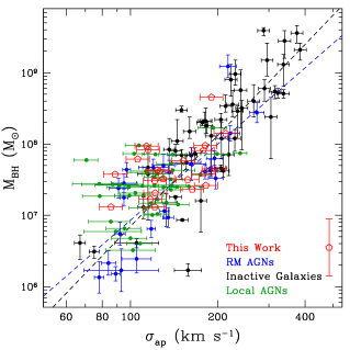
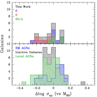
Figure 16.— Left panel: $M_{\rm BH}$-$\sigma$ relation for our sample (red open pentagons), the local RM AGNs (blue; Woo et al., 2010, with the blue dashed line their best fit), and a local sample of AGNs for which $\sigma$ was measured from SDSS (green; Greene & Ho, 2006a) and BH masses taken from Woo et al. (2006). The black datapoints correspond to inactive local galaxies from Gültekin et al. (2009) (with the black dashed line their best fit; see text for details). $\sigma_{\rm ap}$ corresponds to the luminosity-weighted stellar velocity dispersions within a given aperture, depending on the sample (see text for details). The error on the BH mass for both our sample and the local sample of AGNs (green data points) is 0.4 dex and shown as a separate point with error bar in the legend, to reduce confusion of data points. Right panel: Distribution of residuals with respect to the fiducial local relation of Gültekin et al. (2009). Lower panel: literature data; upper panel: our sample (black: full sample; blue: spirals, red: ellipticals, green: S0/a)

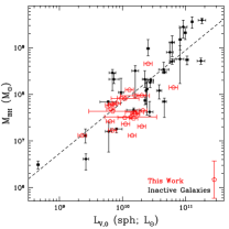
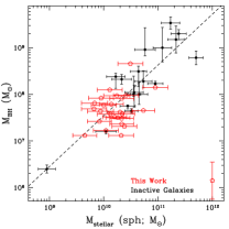
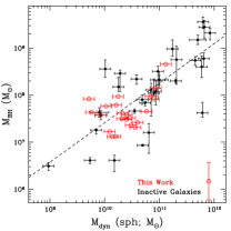
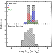
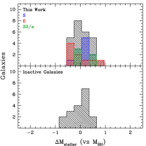
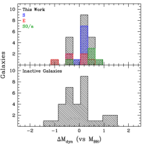
Figure 17.— The same as in Fig. 16, but for the other three $M_{\rm BH}$ scaling relations, namely $M_{\rm BH}$-$L_{\rm sph}$ (left panels), $M_{\rm BH}$-$M_{\rm sph,\star}$ (middle panels), and $M_{\rm BH}$-$M_{\rm sph,dyn}$ (right panels). Left panels: For the $M_{\rm BH}$-$L_{\rm sph}$ relation, we use the local inactive sample from Gültekin et al. (2009), here limited to 35 elliptical and S0 galaxies with a reliable spheroid-disk decomposition. Middle panels: For the $M_{\rm BH}$-$M_{\rm sph,\star}$ relation, stellar masses were calculated from the J, H, and K magnitudes from Marconi & Hunt (2003) for their group 1 (see text for details). Also, BH masses were updated using those listed in Gültekin et al. (2009). Right panels: For the $M_{\rm BH}$-$M_{\rm sph,dyn}$ relation, we compile local inactive galaxies using BH masses from Gültekin et al. (2009), and calculate dynamical masses using $r_{\rm reff,sph}$ given by Marconi & Hunt (2003) and $\sigma_{\rm ap}$ measurements by Gültekin et al. (2009).

Table 7Fits to the Local Scaling Relations

Relation	Sample	$\alpha$	$\beta$	Scatter	Reference
(1)	(2)	(3)	(4)	(5)	(6)
$\log(M_{\rm BH}/M_{\odot})=\alpha+\beta\log(\sigma_{\rm ap}/200{\rm km\,s}^{-1})$	RM AGNs	8$\pm$0.14	3.55$\pm$0.60	0.43$\pm$0.08	Woo+10a
	inactive galaxies	8.12$\pm$0.08	4.24$\pm$0.41	0.44$\pm$0.06	Gültekin+09
$\log(M_{\rm BH}/M_{\odot})=\alpha+\beta\log(L_{\rm sph,V}/10^{11}L_{\odot,V})$	inactive galaxies	8.95$\pm$0.01	1.11$\pm$0.18	0.38$\pm$0.09	Gültekin+09
$\log(M_{\rm BH}/M_{\odot})=\alpha+\beta\log(M_{\rm sph,\star}/M_{\odot})$	inactive galaxies	-3.34$\pm$1.91	1.09$\pm$0.18	0.38$\pm$0.1	here
$\log(M_{\rm BH}/M_{\odot})=\alpha+\beta\log(M_{\rm sph,dyn}/M_{\odot})$	inactive galaxies	-0.98$\pm$1.31	0.84$\pm$0.12	0.54$\pm$0.08	here

Note. — Relations plotted as dashed lines in Figs. 16- 17 and used as fiducial relation when calculating residuals. Col. (1): Scaling relation. Col. (2): Sample used for fitting. (Note that we do not fit our local sample as the scatter is too large.) Col. (3): Mean and uncertainty on the best fit intercept. Col. (4): Mean and uncertainty on the best fit slope. Col. (5): Mean and uncertainty on the best fit intrinsic scatter. Col. (6): References for fit. “here” means determined in this paper independently.

^a Assuming the virial coefficient log f = 0.72$\pm$0.10 (Woo et al., 2010).

7. SUMMARY

To create a local baseline of the BH mass-scaling relations for active galaxies, we selected a sample of $\sim$100 local (0.02 $\leq$ $z$ $\leq$ 0.1) Seyfert-1 galaxies from the SDSS (DR6) with $M_{\rm BH}$ $>10^{7}$M_⊙. All objects were observed with Keck/LRIS, providing us with high-quality longslit spectra. These data allow us to determine, for the first time, spatially-resolved stellar velocity dispersions. Here, we present the methodology and first results of a pilot study of 25 objects. The full sample will be presented in the forthcoming papers of this series.

From the Keck spectra, we measure both spatially-resolved stellar-velocity dispersion and aperture stellar-velocity dispersions in three different spectral regions: around CaHK, around MgIb (after subtraction of underlying broad FeII emission), and around CaT. We present a detailed comparison between spatially-resolved and aperture stellar-velocity dispersions as well as stellar-velocity dispersions from different spectral regions. Also, we determine the width of the H$\beta$ emission line (after subtraction of broad FeII emission and stellar absorption).

On archival SDSS images (g’, r’, i’, z’), we perform surface photometry, using a newly developed code that allows a joint multi-band analysis. We determine the spheroid effective radius, spheroid luminosity, and the host-galaxy free 5100Å AGN continuum luminosity.

Combining the results from spectroscopy and imaging allows us to estimate BH masses via the empirically calibrated photo-ionization method from the width of the H$\beta$ emission line and the host-galaxy free 5100Å AGN continuum luminosity. The spheroid effective radius is used to determine the luminosity-weighted stellar-velocity dispersion within $r_{\rm reff,sph}$. The spheroid luminosities in four different bands are used to calculate stellar masses. Also, our results allow us to estimate dynamical masses. We can thus study four different BH mass scaling relations: $M_{\rm BH}$-$\sigma$, $M_{\rm BH}$-$L_{\rm sph}$, $M_{\rm BH}$-$M_{\rm sph,\star}$, and $M_{\rm BH}$-$M_{\rm sph,dyn}$.

The main results for the pilot study can be summarized as follows.

• The host galaxies show a wide variety of morphologies with a significant fraction of spiral galaxies and prominent rotation curves. This underscores the need for spatially-resolved stellar-velocity dispersions.

• We find a lower merger rate than for our higher redshift study, comparable to inactive galaxies in the local Universe.

• Determining stellar-velocity dispersions from aperture spectra (such as SDSS fiber spectra or unresolved data from distant galaxies) can be biased, depending on the size of the extracted region, AGN contamination, and the host-galaxy morphology. An overestimation of the stellar velocity dispersion from aperture spectra is due to broadening from an underlying rotation component (if seen edge-on), an underestimation can originate from the contribution of the dynamically cold disk (if seen face on). However, comparing with the higher-redshift Seyfert-1 sample of Woo et al. (2008), we find that, on average, such a bias is small ($<$0.03 dex) and, moreover, in the opposite direction to explain the offset seen in the $M_{\rm BH}$-$\sigma$ relation.

• The CaT region is the cleanest region to determine stellar-velocity dispersion in AGN hosts. However, it gets shifted out of the optical wavelength regime to be used beyond redshifts of $z\simeq 0.1$. Alternatively, both the MgIb region, appropriately corrected for FeII emission, and the CaHK region, although often swamped by the blue AGN powerlaw continuum and strong AGN emission lines, can also give accurate results within a few percent, given high S/N spectra. Spatially-resolved data are very helpful to eliminate the AGN contamination by extracting spectra outside of the nucleus.

• The BH mass scaling relations of our pilot sample agree in slope and scatter with those of other local active galaxies as well as inactive galaxies for a canonical choice of the normalization of the virial coefficient.

Appendix A SURFACE PHOTOMETRY

The imaging results of this paper rely on a new surface photometry code that we have developed (§ 4.4). Here we describe the code in detail and discuss the SDSS photometric data and how the code was used to fit surface brightness models to these data.

A.1. SPASMOID: A New Surface Photometry Code

Surface Photometry and Structural Modeling of Imaging Data, or SPASMOID, written by MWA, is an image analysis code designed to supersede the functionality of GALFIT (Peng et al., 2002). The code employs a Bayesian framework wherein the various model parameters (e.g., the centroid, total magnitude, effective radius, ellipticity, position angle, and/or Sérsic index) can be tied together by priors (i.e., constraints) between model components or across different filters. For example, it is straightforward to impose a prior that the redder bands have smaller effective radii than the bluer bands, that the AGN has blue colors related by a power-law of frequency, or that the relative position between the AGN and the bulge is the same in all bands and the offset between these components must be small. The code also allows for a different PSF model for extended objects and point sources (this is useful if the different components have different colors), and can even use linear combinations of PSFs for the AGN to account for PSF-mismatch, which may be particularly important for HST imaging.

The code implements a MCMC sampler to explore degeneracies between the parameters and provide robust error estimates. A set of reduced data images is provided by the user along with variance images, image masks, meta data (e.g., the photometric zeropoints and the pixel scale in each image), and a starting guess for the parameters (this can be substantially different than the best parameters, although a closer guess to the “true” value leads to more efficient sampling). A likelihood function is defined assuming Gaussian uncertainties on the pixel values as described by the variance images, e.g.,

$${\rm log}P=\sum_{\rm images}\sum_{\rm pixels}\frac{({\rm image}-{\rm model})^{2}}{\sigma^{2}_{\rm image}}-\frac{1}{2}{\rm log}2\pi\sigma^{2}_{\rm image}.$$

Priors on all relevant model parameters and – for more complicated models – hyperparameters are defined by the user, and the code uses the PyMC python module to explore the posterior. We have tested our code on simulated and real data and have compared our results with those derived from GALFIT. We find that, for priors that approximate the implicit GALFIT priors, we are able to reproduce the GALFIT results (§ 6.3).

A code as flexible as SPASMOID is ideally suited for space-based data; the spatial resolution and depth of the SDSS photometry limits the utility of such a code, however, it still has its advantages. We now describe how the SDSS data are prepared and subsequently modeled with SPASMOID.

A.2. Preparation of SDSS images

First, we determine the magnitude zeropoint (zp) following the recipe described on the SDSS DR7 webpage:

$$zp=-1\cdot(a+b*{\rm airmass}-2.5\cdot\log({\rm exptime}))$$

with $a$ = zeropoint count rate and $b$ = extinction coefficient taken from the “tsfield” header keywords for a given field and filter, and exptime = 53.91 sec. Then, the sky was subtracted using either the sky value in the image header (if present) or as determined independently directly from the image (note that the 1000-counts bias was also subtracted). We created noise images (in counts) according to

$${\rm noise}=\sqrt{\frac{\rm data+sky}{\rm gain}+\frac{\rm dark\_variance}{\rm gain^{2}}}$$

with data images in counts and gain and dark_variance taken from the “tsfield” header keywords. Then, for convolution with the PSF of the Sloan telescope optics, we use a Gaussian with the parameters given in the “ObjAll” table of SDSS for a given object and filter (“mRrCcPSF_filter”, “mE1PSF_filter”, “mE2PSF_filter”). The average seeing $s$ for the 25 objects was $s_{g}$ = 1.35$\pm$0.15, $s_{r}$ = 1.24$\pm$0.15, $s_{i}$=1.14$\pm$0.15, $s_{z}$=1.16$\pm$0.14.

We only use the four filters g’, r’, i’, and z’, as u’ is generally too faint.

A.3. Running GALFIT for comparison

For comparison, we ran GALFIT on all objects, in a very similar fashion as described in detail in Bennert et al. (2010). In short, we first fit the central AGN component with a PSF, thus determining the center of the system which was subsequently fixed to all components. The PSF used was created as a circular Gaussian with an FWHM corresponding to the seeing, derived from the parameter “mRrCcPSF_filter” by $\sqrt{(}{\rm mRrCcPSF\_filter}/2)*2.355$. We then fitted a two component model only, consisting of a PSF and a de Vaucouleurs (1948) profile. The starting parameters for the GALFIT runs were taken from the SDSS DR7 catalog, i.e. PSF magnitude (“psf_mags”) and de Vaucouleurs (1948) magnitude (“deVmag”) for the spheroid. The minimum radius of the de Vaucouleurs (1948) profile was set to 2 pixels ($\sim$0.8″), i.e. the minimum resolvable size given the seeing.

A.4. Fitting with SPASMOID

Using the GALFIT results (PSF magnitude, location of PSF, spheroid magnitude, spheroid effective radius, ellipticity and position angle) as starting parameters, we assumed the following AGN/host galaxy fitting procedure.

We fit the host galaxy by either a single de Vaucouleurs (1948) profile or by a de Vaucouleurs (1948) plus an exponential profile to account for a disk, while the AGN point source is modeled as the Gaussian described for the convolution PSF in the previous section. All of the components are concentric but the centroids may vary between bands to account for imperfect registration of the images. We also fix the effective radius to be the same in all bands (i.e., our photometry is similar to the modelMag photometry of SDSS) as well as the position angle and axis ratio, although these are free to vary between the bulge and disk component. Again, the minimum radius of the de Vaucouleurs (1948) profile was set to 2 pixels.

The normalizations of the profiles – that is, the magnitudes of each component – are determined by generating models given the structural parameters (centroid, effective radius, axis ratio, and position angle) and finding the best coefficients of a linear fit of these models to the data. In principle the magnitudes could be free parameters of the MCMC sampler, but taking advantage of the linear nature of the fit allows us to very quickly find the ‘optimal’ magnitudes for each proposed set of structural parameters.

Finally, depending on the images, residuals, and the $\chi^{2}$ statistics, we decide whether a given object is best fitted by three components (PSF, spheroid, disk) or two components (PSF + spheroid). (This procedure is similar to the one adopted in Treu et al. 2007 and Bennert et al. 2010.)

We subsequently applied correction for Galactic extinction (subtracting the SDSS DR7 “extinction_filter”’ column). The resulting AB magnitudes were transformed to rest-frame optical bands by performing synthetic photometry on an early-type galaxy template spectrum, a procedure traditionally referred to as k-correction. The template spectrum initially has arbitrary units, and these units were adjusted so that the synthetic observed frame magnitudes match the magnitudes from our photometry. We then evaluated the V-band magnitudes at the rest-frame of the template; luminosities were determined by correcting for the distance modulus given our adopted cosmology. The errors on extinction and rest-frame transformation are a few hundredths of a magnitude. We estimate an uncertainty of $<$0.05 mag (using the scatter in 20 single stellar population templates with ages ranging from 2 Gyr to 8 Gyr). Table 5 summarizes the results.

Note that our model assumes that the host galaxies can be best fitted by either a single de Vaucouleurs (1948) profile or by a de Vaucouleurs (1948) plus an exponential profile. However, some of the spiral galaxies may not have classical bulges, but pseudobulges which are characterized by surface-brightness profiles closer to exponential profiles (e.g., Kormendy & Kennicutt, 2004; Fisher & Drory, 2008). To test the most extreme systematic uncertainties in derived spheroid and PSF magnitude, we re-ran our models for those 14 objects for which we fit a bulge plus disk component using a Sérsic index of $n=1$ instead of $n=4$ for the spheroid component. The results are comparable to what has already been observed by Bennert et al. (2010) (e.g. their Fig. 10b): Decreasing $n$ from 4 to 1 decreases the spheroid luminosity by on average 0.4 mag and increases the nuclear luminosity by on average 0.6 mag. At the same time, the disk luminosity increases by on average 0.1 mag. Thus, the extreme systematic effect would move those objects up in BH mass by on average $\sim$0.1 dex (small, but not negligible compared to the assumed error of 0.4 dex) and towards lower spheroid luminosities by $\sim$0.2 dex. However, the image quality does not allow to determine the best Sérsic index, especially since the objects are complex in nature due to the presence of the AGN for which a perfectly matching PSF fit cannot always be achieved and can result in degeneracies between PSF and spheroid.

A.5. Comparison between GALFIT and SPASMOID Photometry

A comparison between the results from our fit and GALFIT is shown in Figs. 18-19, for the AGN+spheroid decomposition. Overall, the agreement is good, showing that our code performs as expected. In detail, the spheroid magnitudes agree to within 0.01$\pm$0.02 magnitudes (rms scatter: 0.08) with the largest difference at the faint end. For the PSF magnitude, the difference can be larger, due to a fainter PSF compared to the spheroid; on average 0.36$\pm$0.01 (rms scatter: 0.33). We use this comparison for a conservative estimate of our error bars, i.e. spheroid and disk magnitude of 0.2 mag, PSF magnitude of 0.5 mag, and total host magnitude of 0.1 mag. Note that we apply constraints between the different filters which is not the case for GALFIT which is responsible for some of the discrepancies, e.g. in effective radius (Fig. 19). While setting these constraints is less important for an AGN+spheroid fit, it helps to solve the degeneracies for a three component fit. Also, the PSF differs slightly between our code and GALFIT as we use a circular Gaussian for GALFIT but allow for an elliptical Gaussian in our code.

Figure 18.— Comparison between the parameters obtained using GALFIT (G) and SPASMOID (S). First row: Difference between spheroid magnitude determined using GALFIT and SPASMOID as a function of spheroid magnitude (SPASMOID) for the four different SDSS filters. Second row: The same as in the first row, but for the PSF magnitude. Third row: The same as in the second row, but as a function of difference between spheroid and PSF magnitude.

Figure 19.— Comparison between the parameters obtained using GALFIT (G) and SPASMOID (S). First row: Ratio of spheroid effective radius determined by GALFIT vs. SPASMOID as a function of spheroid effective radius determined by SPASMOID for the four different SDSS filters. Note that only for GALFIT is the effective radius different between the four different filters, but the same for all bands in SPASMOID. Second row: The same as in the first row, but for axis ratio b/a. Third row: The same as in the second row, but for position angle.

References

- Auger et al. (2009) Auger, M. W., Treu, T., Bolton, A. S., Gavazzi, R., Koopmans, L. V. E., Marshall, P. J., Bundy, K., & Moustakas, L. A 2009, ApJ, 705, 1099
- Barth et al. (2002) Barth, A. J., Ho, L. C., & Sargent, W. L. W. 2002, AJ, 124, 2607
- Bennert et al. (2010) Bennert, V. N., Treu, T., W. J.-H., Malkan, M. A., Le Bris, A., Auger, M. W., Gallagher, S., & Blandford, R. D. 2010, ApJ, 708, 1507
- Bentz et al. (2006) Bentz, M. C., Peterson, B. M., Pogge, R. W., Vestergaard, M., & Onken, C. A. 2006, ApJ, 644, 133
- Bentz et al. (2009a) Bentz, M. C., Peterson, B. M., Netzer, H., Pogge, R. W., & Vestergaard, M. 2009a, ApJ, 697, 160
- Bentz et al. (2009b) Bentz, M. C., et al. 2009b, ApJ, 705, 199
- Bentz et al. (2009c) Bentz, M. C., et al. 2009c, ApJ, 705, 199
- Bowen (1960) Bowen, I. 1960, ApJ, 132, 1
- Capellari et al. (1996) Capellari, M., Bacon, R., Bureau, M., Damen, M. C., Davies, Roger L., de Zeeuw, P. T., Emsellem, E., Falcón-Barroso, J., Krajnovic, D., Kuntschner, H., McDermid, R. M., Peletier, R. F., Sarzi, M., van den Bosch, R. C. E., & van de Ven, G. MNRAS, 366, 1126
- Ciotti & Ostriker (2007) Ciotti, L., & Ostriker, J. P. 2007, ApJ, 665, L5
- Cristiani & Vio (1990) Cristiani, S. & Vio, R. 1990, A&A 227, 385
- Croton (2006) Croton, D. J. 2006, MNRAS, 369, 1808
- de Vaucouleurs (1948) de Vaucouleurs, G. 1948, Ann. d’Astrophys., 11, 247
- Di Matteo et al. (2008) Di Matteo, T., Colberg, J., Springel, V., Hernquist, L., & Sijacki, D. 2008, ApJ, 676, 33
- Decarli et al. (2010) Decarli, R., Falomo, R., Treves, A., Labita, M., Kotilainen, J. K., & Scarpa, R. 2010, MNRAS, 402, 2453
- Denney et al. (2010) Denney, K. D. et al. 2010, ApJ, 721, 715
- Ferrarese & Merritt (2000) Ferrarese, L., & Merritt, D. 2000, ApJ, 539, L9
- Ferrarese & Ford (2005) Ferrarese, L., & Ford, H. 2005, Space Science Reviews, Volume 116, Issue 3-4, pp. 523-624
- Fisher & Drory (2008) Fisher, D. B., & Drory, N. 2008, AJ, 136, 773
- Francis et al. (1991) Francis, P. J. et al. 1991, ApJ 373, 465
- Gebhardt et al. (2000) Gebhardt, K. et al. 2000, ApJ, 539, L13
- Gebhardt et al. (2003) Gebhardt, K. et al. 2003, ApJ, 583, 92
- Graham et al. (2010) Graham, A. W., Onken, C. A., Athanassoula, E., & Combes, F. 2010, MNRAS submitted (arXiv1007.3834)
- Greene et al. (2010) Greene, J. E., Peng, C. Y., Kim, M., Kuo, C.-Y., Braatz, J. A., Impellizzeri, C. M.V., Condon, J. J., Lo, K. Y., Henkel, C. & Reid, M. J. 2010, ApJ, 721, 26
- Greene & Ho (2006a) Greene, J. E., & Ho, L. C. 2006a, ApJ, 641, L21
- Greene & Ho (2006b) Greene, J. E., & Ho, L. C. 2006b, ApJ, 641, 117
- Greene & Ho (2007) Greene, J. E., & Ho, L. C. 2007, ApJ, 667, 131
- Gu et al. (2009) Gu, M., Chen, Z., & Cao, X. 2009, MNRAS, 397, 3
- Gültekin et al. (2009) Gültekin, K. et al. 2009, ApJ, 698, 198
- Häring & Rix (2004) Häring, N. & Rix, H.-W. 2004, ApJ, 604, L89
- Hickox et al. (2009) Hickox, R. C., et al. 2009, ApJ, 696, 891
- Hopkins et al. (2007) Hopkins, P. F., Hernquist, L., Cox, T. J., Robertson, B., & Krause, E. 2007, ApJ, 669, 45
- Hopkins et al. (2009) Hopkins, P. F., Murray, N., & Thompson, T. A. 2009, MNRAS, 398, 303
- Hopkins et al. (2010) Hopkins, P. F., et al. 2010, ApJ, 715, 202
- Hunt & Malkan (1999) Hunt, L. K. & Malkan, M. A. 1999, ApJ, 516, 660
- Hunt & Malkan (2004) Hunt, L. K. & Malkan, M. A. 2004, ApJ, 616, 707
- Hyde & Bernardi (2009a) Hyde, J. B. & Bernardi, M. 2009a, MNRAS, 396, 1171
- Hyde & Bernardi (2009b) Hyde, J. B. & Bernardi, M. 2009b, MNRAS, 394, 1978
- Jahnke et al. (2004) Jahnke, K., Kuhlbrodt, B., & Wisotzki, L. 2004, MNRAS, 352, 399
- Jahnke et al. (2010) Jahnke, K., et al. 2009, ApJ, 706, 215
- Kaspi et al. (2005) Kaspi, S., Maoz, D., Netzer, H., Peterson, B. M., Vestergard, M. & Jannuzi, B. T. 2005, ApJ, 629, 61
- Kaspi et al. (2000) Kaspi, S., Smith, P. S., Netzer, H., Maoz, D., Jannuzi, B. T. & Giveon, U. 2000, ApJ, 533, 631
- Kauffmann & Haehnelt (2000) Kauffmann, G. & Haehnelt, M. G. 2000, MNRAS, 311, 576
- Kauffmann et al. (2003) Kauffmann, G., et al. 2003, MNRAS, 346, 1055
- Kim et al. (2008) Kim, M., Ho, L. C., Peng, C. Y., Barth, A. J., & Im, M. 2008, ApJS, 179, 283
- Kormendy & Richstone (1995) Kormendy, J., & Richstone, D. 1995, ARA&A, 33, 581
- Kormendy & Kennicutt (2004) Kormendy, J., & Kennicutt, R. C., Jr. 2004, ARA&A, 42, 603
- Li et al. (2008) Li, Z.-Y., Wu, X.-B., & Wang, R. 2008, ApJ, 688, 826
- Malkan et al. (1998) Malkan, M. A., Gorjian, V., & Tam, R. 1998, ApJS, 117, 25
- Malkan et al. (1983) Malkan, M. A. & Filippenko, A. V. 1983, ApJ, 275, 477
- Marconi & Hunt (2003) Marconi, A., & Hunt, L. K. 2003, ApJ, 589, L21
- Marconi et al. (2008) Marconi, A., Axon, D. J., Maiolino, R., Nagao, T., Pastorini, G., Pietrini, P., Robinson, A., & Torricelli, G. 2008, ApJ, 678, 693
- Marconi et al. (2009) Marconi, A., Axon, D. J., Maiolino, R., Nagao, T., Pietrini, P., Robinson, A., & Torricelli, G. 2009, ApJ, 698, 103
- Marziani et al. (2003) Marziani, P., Sulentic, J. W., Zamanov, R., Calvani, M., Dultzin-Hacyan, D., Bachev, R., & Zwitter, T. 2003, ApJS, 145, 199
- McGill et al. (2008) McGill, K. L., Woo, J.-H., Treu, T., & Malkan, M. A. 2008, ApJ, 673, 703
- McLure et al. (2006) McLure, R. J., Jarvis, M. J., Targett, T. A., Dunlop, J. S. & Best, P. N. 2006, MNRAS, 368, 1395
- Merloni et al. (2010) Merloni, A., et al. 2010, ApJ, 708, 137
- Moore (1945) Moore, C. E. 1945, Contributions from the Princeton University Observatory, Vol. 21, page I-I
- Nelson & Whittle (1996) Nelson, C.H. & Whittle, M. 1995, ApJS, 99, 67
- Netzer (2009) Netzer, H. 2009, ApJ, 695, 793
- Netzer (2010) Netzer, H. & Marziani, P. 2010, ApJ, submitted (arXiv1006.3553)
- Neugebauer et al. (1987) Neugebauer, G. et al. 1987, ApJS 63, 615
- Onken et al. (2004) Onken, C. A., Ferrarese, L., Merritt, D., Peterson, B. M., Pogge, R. W., Vestergaard, M., & Wandel, A. 2004, ApJ, 615, 645
- Patton et al. (2002) Patton, D. R., et al. 2002, ApJ, 565, 208
- Peng et al. (2002) Peng, C. Y., Ho, L. C., Impey, C. D., & Rix, H.-W. 2002, AJ, 124, 266
- Peng et al. (2006a) Peng, C. Y., Impey, C. D., Ho, L. C., Barton, E. J., & Rix, H.-W. 2006a, ApJ, 640, 114
- Peng et al. (2006b) Peng, C. Y., Impey, C. D., Rix, H.-W., Kochanek, C. S., Keeton, C. R., Falco, E. E., Lehár, J., & McLeod, B. A. 2006b, ApJ, 649, 616
- Peterson et al. (2004) Peterson, B., Ferrarese, L, Gilbert, K. M., Kaspi, S., Malkan, M. A., Maoz, D., Merritt, D., Netzer, H., Onken, C. A., Pogge, R. W., Vestergaard, M. & Wandel, A. 2004, ApJ, 613, 682
- Riechers et al. (2009) Riechers, D. A., Walter, F., Carilli, C. L., & Lewis, G. F. 2009, ApJ, 690, 463
- Riechers et al. (2008) Riechers, D. A., Walter, F., Brewer, B. J., Carilli, C. L., Lewis, G. F., Bertoldi, F., & Cox, P. 2008, ApJ, 686, 851
- Salviander et al. (2007) Salviander, S., Shields, G. A., Gebhardt, K., & Bonning, E. W. 2007, ApJ, 662, 131
- Shen et al. (2008) Shen, J., Vanden Berk, D. E., Schneider, D. P., & Hall, P. B. 2008, AJ, 135, 928
- Shields et al. (2006) Shields, G. A., Menezes, K. L., Massart, C. A., & Vanden Bout, P. 2006, ApJ, 641, 683
- Suyu et al. (2010) Suyu, S. H., Marshall, P. J., Auger, M. W., Hilbert, S., Blandford, R. D., Koopmans, L. V. E., Fassnacht, C. D., & Treu, T. 2010, ApJ, 711, 201
- Tal et al. (2009) Tal, T., van Dokkum, P. G., Nelan, J., & Bezanson, R. 2009 AJ, 138, 1417
- Treu et al. (2004) Treu, T., Malkan, M. A., & Blanford, R. D. 2004, ApJ, 615, L97
- Treu et al. (2007) Treu, T., Woo, J.-H., Malkan, M. A., & Blanford, R. D. 2007, ApJ, 667, 117
- Vanden Berk et al. (2001) Vanden Berk, D. E. et al. 2001, AJ, 122, 549
- van der Marel & Franx (1993) van der Marel, R. P. & Franx, M. 1993, ApJ, 407, 525
- Vestergaard (2002) Vestergaard, M. 2002, ApJ, 571, 733
- Vestergaard & Peterson (2006) Vestergaard, M. & Peterson, B. M. 2006, ApJ, 641, 689
- Volonteri et al. (2003) Volonteri, M., Haardt, F., & Madau, P. 2003, ApJ, 582, 559
- Walter et al. (2004) Walter, F., Carilli, C., Bertoldi, F., Menten, K., Cox, P., Lo, K. Y., Fan, X., & Strauss, M. A. 2004, ApJ, 615, L17
- Wandel et al. (1999) Wandel, A., Peterson, B. M., & Malkan, M. A. 1999, ApJ, 526, 579
- Weiss et al. (2007) Weiss, A., Downes, D., Neri, R., Walter, F., Henkel, C., Wilner, D. J., Wagg, J. & Wiklind, T. 2007, A&A, 467, 955
- Wyithe & Loeb (2003) Wyithe, J. S., B., & Loeb, A., 2003, ApJ, 595, 614
- Woo & Urry (2002) Woo, J.-H., & Urry, C. M. 2002, ApJ, 579, 530
- Woo et al. (2006) Woo, J.-H., Treu, T., Malkan, M. A., & Blandford, R. D. 2006, ApJ, 645, 900
- Woo et al. (2008) Woo, J.-H., Treu, T., Malkan, M. A., & Blandford, R. D. 2008, ApJ, 681, 925
- Woo et al. (2010) Woo, J.-H., et al. 2010, ApJ, 716, 269
- Zheng et al. (1997) Zheng, W., Kriss, G. A., Telfer, R. C., Grimes, J. P. & Davidsen, A. F. A. 1997, ApJ 475, 469