Staggered and short period solutions of the Saturable Discrete Nonlinear Schrödinger Equation

Abstract

We point out that the nonlinear Schrödinger lattice with a saturable nonlinearity also admits staggered periodic as well as localized pulse-like solutions. Further, the same model also admits solutions with a short period. We examine the stability of these solutions and find that the staggered as well as the short period solutions are stable in most cases. We also show that the effective Peierls-Nabarro barrier for the pulse-like soliton solutions is zero.

The saturable discrete nonlinear Schrödinger equation is increasingly finding applications in various physical situations. Most notably it serves as a model for optical pulse propagation in optically modulated photorefractive media [1], and in this context the pulse dynamics it describes have been intensely studied [2, 3, 4]. In addition to its important role for such applications the saturable discrete nonlinear Schrödinger equation is also of interest from a purely nonlinear science viewpoint [5, 6, 7]. This interest arises because the saturable discrete nonlinear Schrödinger equation has been demonstrated [8] to admit onsite and intersite soliton solutions, which have the same energy. This is contrasted by the standard cubic nonlinear Schrödinger lattice where the onsite solution always has lower energy than the intersite solution. This phenomenon have often been characterized in terms of a so-called Peierls-Nabarro (PN) barrier, which is the energy difference between these two distinct solutions. The particular feature of the saturable discrete nonlinear Schrödinger equation is thus that it allows the PN barrier to change sign and specifically vanish for certain solutions. The vanishing of the PN barrier have been associated with the ability of these solutions to translate undisturbed through the lattice, which is impossible in the cubic discrete nonlinear Schrödinger equation. Here we derive analytical solutions to the saturable discrete nonlinear Schrödinger equation and demonstrate that the localized soliton solutions have a zero PN barrier.

Recently, we obtained [9] two different temporally and spatially periodic solutions to the saturable equation[10]

$$i\dot{\psi}_{n}+(\psi_{n+1}+\psi_{n-1}-2\psi_{n})+\frac{\nu|\psi_{n}|^{2}}{1+\mu|\psi_{n}|^{2}}\psi_{n}=0\,,$$ (1)

where $\psi_{n}$ is a complex valued ‘wavefunction’ at site $n$, while $\nu$ and $\mu$ are real parameters. In particular, the first solution is

$$\psi_{n}^{I}=\frac{1}{\sqrt{\mu}}\frac{\mbox{sn}(\beta,m)}{\mbox{cn}(\beta,m)}\mbox{dn}([n+c]\beta,m)\exp\left(-i[\omega t+\delta]\right),$$ (2)

where the modulus of the elliptic functions $m$ must be chosen such that

$$2-\omega=\frac{\nu}{\mu}=\frac{2\mbox{dn}(\beta,m)}{\mbox{cn}^{2}(\beta,m)},~{}~{}~{}\beta=\frac{2K(m)}{N_{p}}\,,$$ (3)

and $c$ and $\delta$ are arbitrary constants. We only need to consider c between 0 and $\frac{1}{2}$ (half the lattice spacing). Here $K(m)$ denotes the complete elliptic integral of the first kind [11]. The second solution is

$$\psi_{n}^{II}=\sqrt{\frac{m}{\mu}}\frac{\mbox{sn}(\beta,m)}{\mbox{dn}(\beta,m)}\mbox{cn}([n+c]\beta,m)\exp\left(-i[\omega t+\delta]\right)\,,$$ (4)

where the modulus $m$ is now determined such that

$$2-\omega=\frac{\nu}{\mu}=\frac{2\mbox{cn}(\beta,m)}{\mbox{dn}^{2}(\beta,m)},~{}~{}~{}\beta=\frac{4K(m)}{N_{p}}\,.$$ (5)

The integer $N_{p}$ denotes the spatial period of the solutions. In the limit $N_{p}\rightarrow\infty$ ($m\rightarrow 1$), both the solutions $\psi_{n}^{I}$ and $\psi_{n}^{II}$ reduce to the same localized solution

$$\psi_{n}^{III}=\frac{1}{\sqrt{\mu}}\frac{\sinh(\beta)}{\cosh([n+c]\beta)}e^{-i[\omega t+\delta]},~{}~{}(N_{p}\rightarrow\infty),$$ (6)

where $\beta$ is now given by

$$2-\omega=\frac{\nu}{\mu}=2\mbox{cosh}\beta\,.$$ (7)

In Ref. [9], we also developed the stability analysis and examined the linear stability of these solutions to show that the solutions are linearly stable in most cases.

The purpose of this note is to point out that the same model (1) also admits the corresponding staggered solutions. In particular, using the identities for the Jacobi elliptic functions [12], it is easily shown that the model admits the following solutions

$$\psi_{n}^{IS}=(-1)^{n}\frac{1}{\sqrt{\mu}}\frac{\mbox{sn}(\beta,m)}{\mbox{cn}(\beta,m)}\mbox{dn}([n+c]\beta,m)\exp\left(-i[\omega t+\delta]\right)\,,$$ (8)

where the modulus $m$ must be chosen such that

$$\omega-2=-\frac{\nu}{\mu}=\frac{2\mbox{dn}(\beta,m)}{\mbox{cn}^{2}(\beta,m)},~{}~{}~{}\beta=\frac{2K(m)}{N_{p}}\,.$$ (9)

$$\psi_{n}^{IIS}=(-1)^{n}\sqrt{\frac{m}{\mu}}\frac{\mbox{sn}(\beta,m)}{\mbox{dn}(\beta,m)}\mbox{cn}([n+c]\beta,m)\exp\left(-i[\omega t+\delta]\right)\,,$$ (10)

where the modulus $m$ is now determined such that

$$\omega-2=-\frac{\nu}{\mu}=\frac{2\mbox{cn}(\beta,m)}{\mbox{dn}^{2}(\beta,m)},~{}~{}~{}\beta=\frac{4K(m)}{N_{p}}\,.$$ (11)

In the limit $N_{p}\rightarrow\infty$ ($m\rightarrow 1$), both the solutions $\psi_{n}^{IS}$ and $\psi_{n}^{IIS}$ reduce to the same localized staggered solution

$$\psi_{n}^{IIIS}=(-1)^{n}\frac{1}{\sqrt{\mu}}\frac{\sinh(\beta)}{\cosh([n+c]\beta)}e^{-i[\omega t+\delta]},~{}~{}~{}(N_{p}\rightarrow\infty)\,,$$ (12)

where $\beta$ is now given by

$$\omega-2=-\frac{\nu}{\mu}=2\mbox{cosh}\beta\,.$$ (13)

As an illustration we have plotted the exact solutions of the type IS and IIS in Fig. 1. Here the period $N_{p}$ has to be even. We have shown two periods for type IS and only one for type IIS.

There are, as expressed by Eqs. (9), (11), and (13), stringent conditions on the parameters $\mu$ and $\nu$ for which these exact solutions exist. For example, while the nonstaggered solutions are only valid for $\nu>0$ and hence $\omega<2$, the staggered solutions are valid only if $\nu<0$ and hence $\omega>2$. In the case IS the limitation is

$$0~{}(m=1)<-\frac{2\mu}{\nu}<\cos^{2}\left(\frac{\pi}{N_{p}}\right)~{}(m=0)\,,$$ (14)

while in the case IIS the limitation is

$$0~{}(m=1)<-\frac{2\mu}{\nu}<\frac{1}{\cos(\frac{2\pi}{N_{p}})}~{}(m=0)\,.$$ (15)

Similarly, the solution $\psi_{n}^{IIIS}$ exists only when $-\frac{2\mu}{\nu}$ is close to zero (m=1).

We have also examined the linear stability of these solutions and find that the solutions are linearly stable in most cases. A single period $(N=N_{p}$i, where $N$ is the lattice size) is always stable for both solutions IS and IIS. A type IIS solution with more than one period ($N=jN_{p}$, where $j$ is an integer larger than one) is also stable, while a type IS solution with more than one period is always unstable. Thus, the first example in Fig. 1 is in fact unstable.

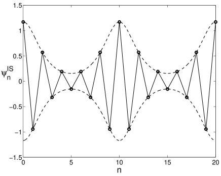
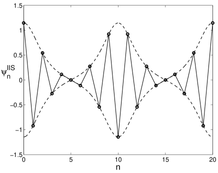
Figure 1: Illustration of the exact solutions of two types. The parameters are: $\nu=-1$, $\mu=0.4$, $\omega=4.5$, and $c=t=\delta=0$. $N_{p}=10$ for $\psi_{n}^{IS}$ and 20 for $\psi_{n}^{IIS}$. The dashed curves represent the solutions given by Eqs. (8) and (10) as if $n$ is a continuous variable. Lines are guides to the eye.

For the solution IIIS, expressions for both the power and the Hamiltonian are identical to those for the solution III and are given by Eqs. (13) and (14) of Ref. [9]. Hence the PN barrier for the solutions III and IIIS is the same. We would like to point out here that the calculation of PN barrier in I was not quite correct. In particular, since both power P and the Hamiltonian H are constants of motion, one must compute the energy difference between the solutions when $c=0$ and $c=1/2$ in such a way that the power P is same in both the cases. On using the expressions for P and H as given by Eqs. (13) and (14) of I, we find that H for the solution III as well as IIIS is given by

$$H=-\frac{4\sinh(\beta)}{\mu}+\frac{2\beta\nu}{\mu^{2}}+2\left(1-\frac{\nu}{2\mu}\right)P\,.$$ (16)

Note that H is in fact independent of $c$, i.e. contrary to our claim in Ref. [9], the PN barrier is in fact zero for our solution III (and hence also for IIIS).

Before completing this note, we would like to mention that the model (1) also admits a few short period solutions.

Using the ansatz

$$\psi_{n}(t)=\phi_{n}e^{-i(\omega t+\delta)}\,,$$ (17)

in Eq. (1) it is easily checked that the only possible short period solutions are to Eq. (1) are:

1. Period 1 solution $\phi_{n}=(...,a,a,...)$ provided

   $$\omega=-\frac{\nu a^{2}}{1+\mu a^{2}}.$$ (18)

2. Period 2 solution $\phi_{n}=(...,a,-a,...)$ provided

   $$\omega=4-\frac{\nu a^{2}}{1+\mu a^{2}}.$$ (19)

3. Period 3 Solution $\phi_{n}=(...,a,0,-a,...)$ provided

   $$\omega=3-\frac{\nu a^{2}}{1+\mu a^{2}}.$$ (20)

4. Period 4 Solutions $\phi_{n}=(...,a,0,-a,0,...)$ and $(...,a,a,-a,-a,...)$ provided

   $$\omega=2-\frac{\nu a^{2}}{1+\mu a^{2}}.$$ (21)

5. Period 6 Solution $\phi_{n}=(...,a,a,0,-a,-a,0,...)$ provided

   $$\omega=1-\frac{\nu a^{2}}{1+\mu a^{2}}.$$ (22)

Applying the stability analysis developed in Ref. [9] we have examined the stability of these short period solutions and find that for a small nonlinearity ($|\nu|<2\mu$) they are all stable. The period 4 solution $(...,a,a,-a,-a,...)$ is always stable while all the other short period solutions possess regions of instabilities at larger nonlinearity. For these low period solutions the stability matrices given by Eqs. (20) and (21) of Ref. [9] are simple and it is, for example, easy to see that the lowest non-zero eigenvalue, $\lambda_{1}(a,\nu)$, of the stability problem for the period 1 solutions is given by ($\mu=1$)

$$\lambda_{1}(a,\nu)=a^{4}+\left(2-\frac{2}{3}\nu\right)a^{2}+1.$$ (23)

Similarly, we have for the period 2 solution

$$\lambda_{2}(a,\nu)=a^{4}+\left(2+\frac{2}{3}\nu\right)a^{2}+1,$$ (24)

and the period 4 solution

$$\lambda_{4}(a,\nu)=a^{4}+(2-|\nu|)a^{2}+1.$$ (25)

These expressions correspond to the relevant curves in Fig. 2.

It possible to derive similar expressions for the period 3 and period 6 solutions but the expressions are more complicated and will be omitted here.

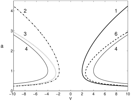
Figure 2: Regions of stability for the short period solutions to Eq. (1) for $\mu=1$. Period 1: thick full curve, period 2: dashed-dotted curve, period 3: long-dashed curve, period 4: thin full curve, and period 6: short-dashed curve. The instability occurs in the parameter region encompassed by the respective curves.

Clearly the $p$ period solutions are unstable for the parameter values where $\lambda_{p}(a,\nu)<0$, and we have illustrated these regions in Fig. 2. Figure 2 shows the curves in the $(a,\nu)$-plane where $\lambda_{p}(a,\nu)=0$ so that the instability occurs in the regions that are encompassed by the respective curves. A symmetry is apparent in this stability diagram and it is easy to realize that this symmetry arises from the fact that the transformation $(\nu,\phi_{n})\rightarrow(-\nu,(-1)^{n}\phi_{n})$ establishes the following connection between the short period solutions: 1 $\leftrightarrow$ 2, 3 $\leftrightarrow$ 6, and 4 $\leftrightarrow$ 4.

In conclusion, we have obtained staggered as well as short period solutions of the saturable discrete nonlinear Schrödinger equation. We also studied the linear stability and found the solutions to be stable in certain parameter ranges. Finally, we found that the Peierls-Nabarro barrier for the pulse solutions is zero. Our results are relevant to optical soliton pulse propagation in waveguides and photorefractive media [1].

Research at Los Alamos National Laboratory is carried out under the auspices of the National Nuclear Security Administration of the U.S. Department of Energy under Contract No. DE-AC52-06NA25396.

References

- [1] Fleischer J.W. 2005 Opt. Express 13 1780.
- [2] Fitrakis E.P., Kevrekidis P.G., Malomed B.A., and Frantzeskakis, D.J. 2006 Phys. Rev. E 74, 026605.
- [3] Vicencio R.A. and Johansson M 2006 Phys. Rev. E 73, 046602.
- [4] Cuevas J and Eilbeck J.C. 2006 Phys. Lett. A 358, 15.
- [5] Melvin T.R.O., Champneys A.R., Kevrekidis P.G. 2006 Phys. Rev. Lett. 97, 124101.
- [6] Oxtoby O.F., Barashenkov I.V. 2007 Phys. Rev. E, 76, 036603.
- [7] Melvin T.R.O, Champneys A.R., Kevrekidis P.G. 2008 Physica D 237, 551.
- [8] L. Hadzievskii, A. Maluckov, M. Stepic, D. Kip 2004 Phys. Rev. Lett. 93, 033901.
- [9] Khare A., Rasmussen K.Ø, Samuelsen M.R., and Saxena A. 2005 J. Phys. A38, 807; hereafter we will refer to it as I.
- [10] Note that rewritting and the notation change followed by the gauge transformation render the equantion in a perhaps more often used form [7].
- [11] Handbook of Mathematical Functions with Formulas, Graphs, and Mathematical Tables, edited by M. Abramowitz and I. A. Stegun (U.S. GPO, Washington, D.C., 1964).
- [12] Khare A. and Sukhatme U. 2002 J. Math. Phys. 43, 3798; Khare A., Lakshminarayan A., Sukhatme U 2003 J. Math. Phys. 44, 1822; math-ph/0306028; 2004 Pramana (Journal of Physics) 62, 1201.