Exact Solutions of the Two-Dimensional Discrete Nonlinear Schrödinger Equation with Saturable Nonlinearity

Abstract

We show that the two-dimensional, nonlinear Schrödinger lattice with a saturable nonlinearity admits periodic and pulse-like exact solutions. We establish the general formalism for the stability considerations of these solutions and give examples of stability diagrams. Finally, we show that the effective Peierls-Nabarro barrier for the pulse-like soliton solution is zero.

I Introduction.

The discrete nonlinear Schrödinger equation (DNLSE) finds widespread use in physics due to its very general nonlinear character. It arises in the context of the propagation of electromagnetic waves in optical waveguides emwave , and it also appears in the study of Bose-Einstein condensates in optical lattices bec . Recently we have studied the exact soliton solutions and their stability for the one-dimensional DNLSE with a saturable nonlinearity krss1 . We were also able to obtain staggered and short period solutions of this equation krss2 as well as to generalize our results to arbitrarily higher-order nonlinearities krsss .

Two-dimensional periodic lattices with a saturable nonlinearity in the Schrödinger equation have been experimentally realized in photorefractive materials efrem . Solitons have also been observed in these crystals fleischer ; martin . Localized traveling wave solutions that exist only for finite velocities have been computed in this case melvin . The question of discrete soliton mobility in these systems has been addressed as well magnus . Here we show that it is also possible to obtain exact periodic and pulse-like soliton solutions for the two-dimensional DNLSE with a saturable nonlinearity. We then study the stability of these solutions as a function of the parameters of the equation. We also show that similar to the one dimensional case, the effective Peierls-Nabarro barrier (i.e. the discreteness barrier for soliton motion) for the pulse-like soliton solutions is zero. In addition, we find several short period solutions.

II Two-dimensional discrete nonlinear Schrödinger equation with saturable nonlinearity.

The equation we consider is the following asymmetric, DNLSE with a saturable nonlinearity in two dimensions

$$i\frac{d\phi_{n,m}}{dt}+[\zeta(\phi_{n+1,m}+\phi_{n-1,m})+\xi(\phi_{n,m+1}+\phi_{n,m-1})]+\frac{\nu|\phi_{n,m}|^{2}\phi_{n,m}}{1+|\phi_{n,m}|^{2}}=0\,.$$ (1)

$|\zeta-\xi|$ is a measure of the spatial asymmetry and $\nu$ a measure of the nonlinearity. This equation can be derived from the Hamiltonian

$$H=\sum_{n,m=1}^{N,M}\bigg{[}\zeta|\phi_{n+1,m}-\phi_{n,m}|^{2}+\xi|\phi_{n,m+1}-\phi_{n,m}|^{2}$$

$$-[2(\zeta+\xi)+\nu]|\phi_{n,m}|^{2}+\nu\ln(1+|\phi_{n,m}|^{2})\bigg{]}\,,$$ (2)

and the equation of motion being derived from

$$i\dot{\phi}_{n,m}=\frac{\partial H}{\partial\phi_{n,m}^{*}},$$ (3)

considering $\phi_{n,m}$ and $i\phi_{n,m}^{*}$ as conjugate variables. There are two conserved quantities for the field equation, Eq. (1), the Hamiltonian $H$ and the power (norm) $P$ defined by

$$P=\sum_{n,m=1}^{N,M}|\phi_{n,m}|^{2}\,.$$ (4)

Note that the system is invariant under simultaneous interchange of $\zeta$ and $\xi$, and $n$ and $m$.

III Exact solutions to the two-dimensional equation.

Exact stationary solutions can also be obtained in the case of this two-dimensional discrete, asymmetric saturable nonlinear Schrödinger equation (1). We are looking for stationary solutions using the ansatz

$$\phi_{n,m}(t)=u_{n,m}e^{-i(\omega t+\delta)}\,,$$ (5)

and obtain from Eq. (1), the following difference equation

$$(1+u_{n.m}^{2})\omega u_{n,m}+(1+u_{n,m}^{2})[\zeta(u_{n+1,m}+u_{n-1,m})+\xi(u_{n,m+1}+u_{n,m-1})]+\nu u_{n,m}^{3}=0\,.$$ (6)

Following Ref. krss1 we immediately find two different types of solutions. One that is symmetric in $n$ and $m$ and one that only depends on $n$ (and by symmetry one that only depends on $m$).

Symmetric case:

If one chooses

$$\omega=-\nu\,,$$ (7)

then

$$u_{n,m}^{s}=\frac{{\rm sn}(\beta,k)}{{\rm cn}(\beta,k)}{\rm dn}(\beta(n+m+\delta_{1}),k)\,,$$ (8)

is a solution if $k$ is chosen to fulfill

$$\frac{\nu}{\zeta+\xi}=2\frac{{\rm dn}(\beta,k)}{{\rm cn}^{2}(\beta,k)}\,,~{}~{}\beta=\frac{2K(k)}{N_{p}}\,.$$ (9)

Similarly

$$u_{n,m}^{s}=k\frac{{\rm sn}(\beta,k)}{{\rm dn}(\beta,k)}{\rm cn}(\beta(n+m+\delta_{1}),k)\,,$$ (10)

is a solution provided

$$\frac{\nu}{\zeta+\xi}=2\frac{{\rm cn}(\beta,k)}{{\rm dn}^{2}(\beta,k)}\,,~{}~{}\beta=\frac{4K(k)}{N_{p}}\,.$$ (11)

Here $k$ is the elliptic modulus (the elliptic parameter $m=k^{2}$ stegun ) of the Jacobi elliptic functions ${\rm sn}(x,k)$, ${\rm cn}(x,k)$, and ${\rm dn}(x,k)$ and $K(k)$ is the complete elliptic integral of the first kind stegun ; Ryzhik . The integer $N_{p}$ denotes the spatial period of the system. $N$ and $M$ in Eq. (II) must be chosen as multiples of $N_{p}$. The two solutions have a common pulse-like limit for $k\rightarrow 1$ (and $N_{p}\rightarrow\infty$),

$$u_{n,m}^{s}=\sinh(\beta){\rm sech}[\beta(n+m+\delta_{1})]\,,$$ (12)

which is a solution if $\beta$ fulfills

$$\frac{\nu}{\zeta+\xi}=2\cosh(\beta)\,.$$ (13)

By symmetry, a change of sign of $n$ (or $m$) in Eqs. (8), (10), and (12) will give solutions with exactly the same properties.

Asymmetric case:

If one chooses for the frequency

$$\omega=-\nu-2\xi\,,$$ (14)

then

$$u_{n,m}^{as}=\frac{{\rm sn}(\beta,k)}{{\rm cn}(\beta,k)}{\rm dn}(\beta(n+\delta_{1}),k)\,,$$ (15)

will be a solution for $k$ satisfying

$$\frac{\nu}{\zeta}=2\frac{{\rm dn}(\beta,k)}{{\rm cn}^{2}(\beta,k)}\,,~{}~{}\beta=\frac{2K(k)}{N_{p}}\,.$$ (16)

Similarly, we also have a $cn$ solution.

$$u_{n,m}^{as}=k\frac{{\rm sn}(\beta,k)}{{\rm dn}(\beta,k)}{\rm cn}(\beta(n+\delta_{1}),k)\,,$$ (17)

provided

$$\frac{\nu}{\zeta}=2\frac{{\rm cn}(\beta,k)}{{\rm dn}^{2}(\beta,k)}\,,~{}~{}\beta=\frac{4K(k)}{N_{p}}\,.$$ (18)

Here $N=N_{p}$ and $M$ can be any integer.
Again both these solutions approach the pulse solution in the limit $k\rightarrow 1$ and $N_{p}\rightarrow\infty$

$$u_{n,m}^{as}=\sinh(\beta){\rm sech}[\beta(n+\delta_{1})]\,,$$ (19)

provided

$$\frac{\nu}{\zeta}=2\cosh(\beta)\,.$$ (20)

Another asymmetric solution appears if we interchange $n$ and $m$ and $\zeta$ and $\xi$ ($M=N_{p}$ and $N$ any integer). We note that, in all cases, changing the sign of $\xi$ is equivalent to staggering the solution in the $m$ direction ($(-1)^{m}$ as an amplitude factor) and changing the sign of $\zeta$ is equivalent to staggering the solution in the $n$ direction krss2 .

The described solutions are in some sense direct generalizations of our earlier results for the one-dimensional version of the saturable nonlinear Schrödinger equation, since they remain spatially uniform along a specific direction in space. Such solutions are well-known for nonlinear partial differential equations and are often, in such a continuum setting, referred to as line solutions or line solitons. However, in continuum settings, such solutions are generally not stable, because the extra dimension now allows for an entire set of new instability modes to come into play. In our discrete case, however, we shall demonstrate that these solutions indeed can be stable in certain cases. The fact that these solutions have infinite extension along one of their dimensions probably renders them less physically important. However, their stability analysis does, as we will demonstrate, give detailed insight into the intricate stability mechanisms of this nonlinear system. Specifically, are the parameters $(\nu,\xi)$, which control the stability, directly related to materials properties such as the change in refractive index of the crystal.

IV Stability of the solutions.

In order to study the linear stability of these exact solutions $u_{n,m}^{j}$ ($j$ is “s” (symmetric) or “as” (asymmetric)) we introduce the following expansion around the exact solution

$$\phi_{n,m}(t)=u_{n,m}^{j}e^{-i(\omega t+\delta)}+\delta u_{n,m}(t)e^{-i(\omega t+\delta)}$$ (21)

applied in a frame rotating with frequency $\omega$ of the solution. Substituting (21) into the field equation, Eq. (1), and retaining only terms linear in the deviation, $\delta u_{n,m}$, we get

$$i\delta\dot{u}_{n,m}+\zeta\big{(}\delta u_{n+1,m}+\delta u_{n-1,m}\big{)}+\xi\big{(}\delta u_{n,m+1}+\delta u_{n,m-1}\big{)}+\left(\omega+\frac{\nu|u_{n,m}^{j}|^{2}(2+|u_{n,m}^{j}|^{2})}{(1+|u_{n,m}^{j}|^{2})^{2}}\right)\delta u_{n,m}+\frac{\nu|u_{n,m}^{j}|^{2}}{(1+|u_{n,m}^{j}|^{2})^{2}}\delta u_{n,m}^{*}=0.$$ (22)

We continue by splitting the deviations $\delta u_{n,m}$ into real parts $\delta u_{n,m}^{(r)}$ and imaginary parts $\delta u_{n,m}^{(i)}$ ($\delta u_{n,m}=\delta u_{n,m}^{(r)}+i\delta u_{n,m}^{(i)}$) and introducing the two real vectors

$$\delta\mbox{\boldmath$U^{r}$}=\{\delta u_{n,m}^{(r)}\}=\{\delta U_{J}^{(r)}\}, \delta\mbox{\boldmath$U^{i}$}=\{\delta u_{n,m}^{(i)}\}=\{\delta U_{J}^{(i)}\},$$ and (23)

where the pair of indices $m,n$ are replaced by a single index $J$ via: $J=n+(m-1)N_{p}$. By introducing the real matrices $\mbox{\boldmath$A$}=\{A_{J,J^{\prime}}\}$ and $\mbox{\boldmath$B$}=\{B_{J,J^{\prime}}\}$ defined by

$$A_{J,J^{\prime}}=\zeta(\delta_{J,J^{\prime}+1}+\delta_{J,J^{\prime}-1})+\xi(\delta_{J,J^{\prime}+N_{p}}+\delta_{J,J^{\prime}-N_{p}})+\left(\omega+\frac{\nu|u_{n,m}^{j}|^{2}(3+|u_{n,m}^{j}|^{2})}{(1+|u_{n,m}^{j}|^{2})^{2}}\right)\delta_{J,J^{\prime}},$$ (24)

$$B_{J,J^{\prime}}=\zeta(\delta_{J,J^{\prime}+1}+\delta_{J,J^{\prime}-1})+\xi(\delta_{J,J^{\prime}+N_{p}}+\delta_{J,J^{\prime}-N_{p}})+\left(\omega+\frac{\nu|u_{n,m}^{j}|^{2}}{(1+|u_{n,m}^{j}|^{2})}\right)\delta_{J,J^{\prime}}~{}~{}~{}~{}~{}~{}~{}~{}~{}~{}$$ (25)

where $J^{\prime}\pm 1$ and $J^{\prime}\pm N_{p}$ in the Kronecker $\delta$ means: $J^{\prime}\pm 1~{}mod~{}N_{p}$ and $J^{\prime}\pm N_{p}~{}mod~{}N_{p}$ to ensure periodic boundary conditions, Eq. (22) becomes

$$-\delta\mbox{\boldmath$\dot{U^{i}}$}+\mbox{\boldmath$A$}\delta\mbox{\boldmath$U^{r}$}=\mbox{\boldmath$0$}, \delta\mbox{\boldmath$\dot{U^{r}}$}+\mbox{\boldmath$B$}\delta\mbox{\boldmath$U^{i}$}=\mbox{\boldmath$0$}.$$ and (26)

Combining these first order differential equations we get:

$$\delta\mbox{\boldmath$\ddot{U^{i}}$}+\mbox{\boldmath$A$}\mbox{\boldmath$B$}\delta\mbox{\boldmath$U^{i}$}=\mbox{\boldmath$0$}, \delta\mbox{\boldmath$\ddot{U^{r}}$}+\mbox{\boldmath$B$}\mbox{\boldmath$A$}\delta\mbox{\boldmath$U^{r}$}=\mbox{\boldmath$0$}.$$ and (27)

The two matrices $A$ and $B$ are symmetric and have real elements. However, since they do not commute $A$$B$ and $\mbox{\boldmath$B$}\mbox{\boldmath$A$}=(\mbox{\boldmath$A$}\mbox{\boldmath$B$})^{tr}$ are not symmetric. $A$$B$ and $B$$A$ have the same eigenvalues, but different eigenvectors. The eigenvectors for each of the two matrices need not be orthogonal. The eigenvalue spectrum $\{\gamma\}$ of the matrix $A$$B$ (or $B$$A$) determines the stability of the exact solutions. If $\{\gamma\}$ contains negative eigenvalues then the solution is unstable. The eigenvalue spectrum always contains two eigenvalues which are zero. These eigenvalues correspond to the translational invariance in space and time (represented by $\delta_{1}$ and $\delta$). The given solutions are unstable for most of the parameter space $(\zeta,\xi,\nu)$. From Ref. krss1 we know that $\xi=0$ generally leads to stable solutions. In determining the stability of the solutions it is useful to note that the rescaling transformation $(\zeta,\xi,\nu)\rightarrow\alpha(\zeta,\xi,\nu)$ ($\omega\rightarrow\alpha\omega$) changes the eigenvalues by $\alpha^{2}$ and therefore it does not affect the stability (i.e. the sign of eigenvalues) of the solutions. Therefore the three-dimensional parameter space $(\zeta,\xi,\nu)$ can be significantly reduced (into a two-dimensional parameter space) as far as stability considerations are concerned. The nonlinearity parameter $\nu\neq 0$, separates the three-dimensional parameter space into two disconnected equivalent ones for $\nu>0$ and $\nu<0$, respectively. The rescaling transformation with $\alpha=-1$ interchanges the two equivalent half spaces. So we need only to consider positive $\nu$. From here on we treat the symmetric and the asymmetric cases separately.

Stability of the symmetric case:

Since $\nu>0$, Eqs. (9), (11), and (13) require $\zeta+\xi>0$ and therefore $\zeta>-\xi$. Further, we can always choose $\zeta>\xi$ due to the inter-changeability of $\zeta$ and $\xi$. We therefore have $-\zeta<\xi<\zeta$ or applying the scaling condition $-1<\xi/\zeta<1$. This means that the stability of the entire parameter space can be mapped out onto the much smaller parameter space $(1,\xi,\nu)$, where $-1<\xi<1$ (and $\nu>0$).

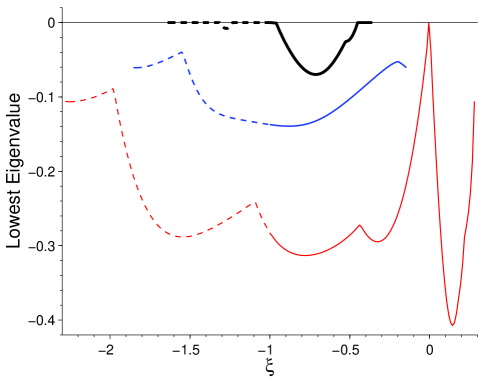
Figure 1: Stability analysis for the $dn$ solution, Eq. (8). Lowest eigenvalues for $|\nu|=1.5$ (thick line, black online), $|\nu|=2$ (medium thick line, blue online), and $|\nu|=3$ (thin line, red online). Dashed (solid) lines indicate negative (positive) values of $\nu$. Stability occurs when the lowest eigenvalue is zero. The entire existence interval is shown for positive $\nu$. Negative $\nu$ results can be obtained by rescaling the results for positive $\nu$. The remaining parameters are: $\zeta=1$ and $N_{p}=8$.

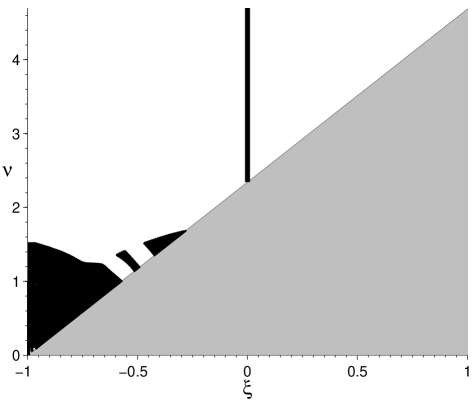
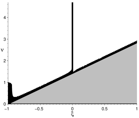
Figure 2: General stability diagram for symmetric $dn$ (left) and $cn$ (right) solutions of Eq. (8) and Eq. (10), respectively. In the grey region no solution of the given kind exists. In the white regions solutions are unstable, while the black area indicates stable solutions. The vertical line $\xi=0$, which represents the one-dimensional stability result, is part of the black area. The rough or jagged appearance of parts of the stability boundary is due to limited numerical resolution rather than an intrinsic feature of the problem. Parameters are: $\zeta=1$, and $N_{p}=8$.

In Fig. 1 we illustrate the stability analysis for the $dn$ solution, Eq. (8), by showing the lowest eigenvalue as a function of $\xi$ for several values of $\nu$. Stability occurs whenever the lowest eigenvalue is zero. The entire existence regime is illustrated for positive $\nu$ and a few windows of stability can be seen. It is important to note that the results for negative values of $\nu$ ($\xi<-1$) are superfluous as they can be obtained by rescaling the results for positive $\nu$. To demonstrate this we have for $\zeta=1$: $(1,-|\xi|,-|\nu|)\rightarrow(-1/|\xi|,1,|\nu|/|\xi|)\rightarrow(1,-1/|\xi|,|\nu|/|\xi|)$ where the last step follows by the inter-changeability of the two-coupling parameters. This shows that the $\nu<0$ regime can be mapped onto the $\nu>0$ regime. Generally, stability is only observed for $\xi<0$. This means that stability for the symmetric ${\rm dn}$ solutions can only be achieved when $\xi$ and $\zeta$ have opposite signs. Recalling the equivalence between staggered solutions and sign changes of $\xi$ or $\zeta$, another way to view this result is that the symmetric ${\rm dn}$ solutions must be staggered in one dimension when $\zeta$ and $\xi$ are both positive in order to be stable. This is clearly a property arising from the discreteness that cannot be achieved in a continuum system.

Assembling results like those shown in Fig. 1 for a range of $\nu$ and $\xi$ values we arrive at Fig. 2 where stability diagrams for both the $dn$ and the $cn$ solutions to Eq. (8) and Eq. (10), respectively, are shown. The grey region indicates that the solutions do not exist, whereas the black (white) regions indicate the existence of stable (unstable) solutions. These two stability diagrams have a very similar structure. However, the $cn$ solutions are always stable in the proximity of the existence boundary marked by the grey area. This property is related to the fact that the amplitude (which is $\propto k$, see Eq.(10)) of this solution vanishes at the existence boundary where $k=0$. Also, we note that the common pulse solution corresponds to the corner close to $(\xi,\nu)=(-1,0)$.

We have looked at other values of $N_{p}$ and find that for larger $N_{p}$, the stability diagram has similar features. The pulse-like solution only exists in the limit $N_{p}\rightarrow\infty$, and here it has the same stability properties as the $dn$ and $cn$ solutions for $k\rightarrow 1$. Therefore, our analysis indicates that the symmetric pulse-like solutions are stable for small $\nu$ and $\xi\sim-1$.

Stability of the asymmetric case:

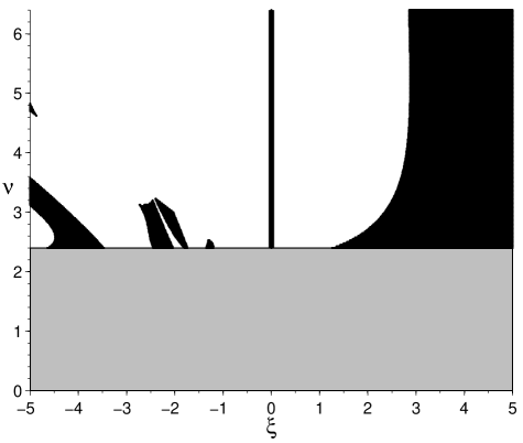
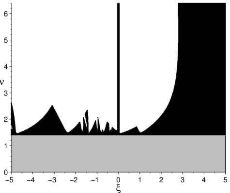
Figure 3: General stability diagram for the asymmetric $dn$ (left) and $cn$ (right) solutions of Eq. (15) and Eq. (17), respectively. In the grey region no solution of the given kind exists. In the white region solutions are unstable, while the black area indicates stable solutions. The vertical line $\xi=0$, which represents the one-dimensional stability result, is part of the black area. Parameters are: $\zeta=1$, and $N_{p}=8$.

We proceed almost as in the symmetric case. We still have $\nu>0$, therefore from Eqs. (16), (18), and (20) we have $\zeta>0$. So here the three-dimensional parameter space can be reduced to $(1,\xi,\nu)$, where $-\infty<\xi<\infty$ (and $\nu>0$). Illustrations of the stability diagrams are given for the asymmetric $dn$ and $cn$ solutions, Eq. (15) and Eq. (17), respectively in Fig. 3 for $\zeta=1$ and $N_{p}=8$. Again the two stability diagrams have a very similar structure except that the parameter space for stability of the asymmetric solution is much larger. As in the symmetric case, even in the asymmetric case, the $cn$ solutions are always stable in the proximity of the existence boundary marked by the grey area. Here we note that the common pulse solution corresponds to large $\nu$ and $\xi$.

V Peierls-Nabarro barrier for the pulse solution

We would now like to show the absence of Peierls-Nabarro barrier for the pulse solution. However, we must remember that since both power $P$ and Hamiltonian $H$ are constants of motion, one must compute the energy difference between the solutions when $\delta_{1}=0$ and $\delta_{1}=1/2$ in such a way that the power $P$ is same in both the cases.

For the pulse solution obtained above, the power $P$ is given by

$$P=\sum_{n,m=-\infty}^{\infty}|\phi_{n,m}|^{2}=\sinh^{2}(\beta)\sum_{n,m=-\infty}^{\infty}{\rm sech}^{2}[\beta(n+m+\delta_{1})]\,.$$ (28)

This double sum can be evaluated using the single sum result

$$\sum_{n=-\infty}^{\infty}{\rm sech}^{2}[\beta(n+\delta_{2})]=\frac{2}{\beta}+\frac{2K(k)E(k)}{\beta^{2}}+\left(\frac{2K(k)}{\beta}\right)^{2}{\rm dn}^{2}[2\delta_{2}K(k),k]\,,$$ (29)

the above $P$ is given by

$$P=\sum_{m=-\infty}^{\infty}\sinh^{2}(\beta)\left[\frac{2}{\beta}+\frac{2K(k)E(k)}{\beta^{2}}+\left(\frac{2K(k)}{\beta}\right)^{2}{\rm dn}^{2}[2(m+\delta_{1})K(k),k]\right]\,.$$ (30)

Note, only the last term on the rhs is $m$ dependent. In these equations $E(k)$ is the complete elliptic integral of the second kind.

Let us now discuss the computation of the Hamiltonian $H$. Clearly, for the pulse solution obtained above, $H$ as given by Eq. (II) takes the form

$$H=\sum_{n,m=-\infty}^{\infty}\bigg{[}-\nu P+\nu\ln[1+\sinh^{2}(\beta){\rm sech}^{2}(\beta[n+m+\delta_{1}])]$$

$$-2\sinh^{2}(\beta)[{\rm sech}(\beta[n+1+m+\delta_{1}]){\rm sech}(\beta[n+m+\delta_{1}])(\zeta+\xi)]\bigg{]}\,.$$ (31)

Again we use the single sum results to evaluate the double sum, i.e.

$$\sum_{n=-\infty}^{\infty}\big{[}{\rm sech}[\beta(n+1+\delta_{2})]{\rm sech}[\beta(n+\delta_{2})]\big{]}=\frac{2}{\sinh(\beta)}\,,$$ (32)

$$\sum_{n=-\infty}^{\infty}\ln[1+\sinh^{2}(\beta){\rm sech}^{2}(\beta[n+\delta_{2}])]=2\beta\,,$$ (33)

the above $H$ is given by

$$H=\sum_{m=-\infty}^{\infty}\bigg{[}-\nu P+2\nu\beta-4(\zeta+\xi)\sinh(\beta)\bigg{]}\,.$$ (34)

We thus note that for a given power $P$ (which contains a sum over $m$), H is indeed independent of $\delta_{1}$, i.e. the Peierls-Nabarro barrier is indeed zero for the pulse solution. The same holds true for the asymmetric solution.

VI Short period solutions

Recently we obtained short period solutions to the one-dimensional saturable DNLSE krss2 . These short period ($N$) solutions, in the one-dimensional case, can be written in the following compact form (coming from equally distributed points on a circle so that projection on the $x$-axis should only be 0 or $\pm a$):

$$u_{N}(n)=\frac{a}{\cos(\varphi_{N})}\cos\left(\frac{2\pi n}{N}+\varphi_{N}\right),$$ (35)

where $\varphi_{1}$ =$\varphi_{2}$ =$\varphi_{4s}=0$, (4s is the stable period 4) and $\varphi_{4}=\frac{\pi}{4}$, $\varphi_{3}=\varphi_{6}=\frac{\pi}{6}$.

$$u_{N}(n+1)+u_{N}(n-1)=\frac{a}{\cos(\varphi_{N})}\bigg{[}\cos\left(\frac{2\pi(n+1)}{N}+\varphi_{N}\right)+\cos\left(\frac{2\pi(n-1)}{N}+\varphi_{N}\right)\bigg{]}$$ (36)

$$=\frac{2a}{\cos(\varphi_{N})}\cos\left(\frac{2\pi n}{N}+\varphi_{N}\right)\cos\frac{2\pi}{N}=2\psi_{N}(n)\cos\frac{2\pi}{N}.$$ (37)

For $\omega$ we get

$$\omega=-2\zeta\cos\frac{2\pi}{N}-\frac{\nu a^{2}}{1+a^{2}}.$$ (38)

Assuming that in the two-dimensional case, the solution is a product of the two one-dimensional solutions (with period $N$ and period $M$), i.e.

$$u_{N,M}(n,m)=\frac{a}{\cos(\varphi_{N})\cos(\varphi_{M})}\cos\left(\frac{2\pi n}{N}+\varphi_{N}\right)\cos\left(\frac{2\pi m}{M}+\varphi_{M}\right),$$ (39)

we get:

$$\omega=-2\zeta\cos\frac{2\pi}{N}-2\xi\cos\frac{2\pi}{M}-\frac{\nu a^{2}}{1+a^{2}}.$$ (40)

VII Conclusions

We have given analytical expressions for the solutions to the two-dimensional discrete nonlinear Schrödinger equation with saturable nonlinearity which arises in photorefractive crystals efrem ; fleischer ; martin ; melvin ; magnus . Due to their infinite extension along one of their dimensions, these solutions are not very physically meaningful but it is very rare that solutions to discrete nonlinear two-dimensional problems can be described in closed form using standard mathematical functions as we have done here. This feature of the solutions is physically significant because it provides an opportunity for in-depth scrutiny and understanding that is not usually available in a nonlinear physical system. These solutions are closely related to the previously derived krss1 solutions to the corresponding one-dimensional equation. However, in contrast to what one may expect based on intuition derived from similar nonlinear partial differential equations, we have shown that these solutions are linearly stable in certain regions of the parameter space. Specifically, we have observed that the asymmetric versions of these solutions lead to a very intricate stability diagram. We have shown that the symmetric $dn$ solution is stable in certain regions of the parameter space provided it is staggered in one dimension. However, the symmetric $cn$ solution as well as the asymmetric $cn$ and $dn$ solutions are stable in certain regions of parameter space both when they are non-staggered or if they are staggered in one dimension. The finding that nonlinear waveforms in two-dimensional photorefractive materials best achieve stability in the presence of phase asymmetry between the two spatial directions is crucial because the photonic lattices that represent the physical realization of Eq.(1) tend to naturally possess this property OL . Finally, we found that the Peierls-Nabarro barrier for the pulse solution is zero. An understanding of the mobility of these exact discrete two-dimensional solutions remains an important issue magnus .