A Theory of Mulicolor Black Body Emission from Relativistically Expanding Plasmas

Abstract

We consider the emission of photons from the inner parts of a relativistically expanding plasma outflow, characterized by a constant Lorentz factor, $\Gamma$. Photons that are injected in regions of high optical depth are advected with the flow until they escape at the photosphere. Due to multiple scattering below the photosphere, the locally emerging comoving photon distribution is thermal. However, as an observer sees simultaneously photons emitted from different angles, hence with different Doppler boosting, the observed spectrum is a multi-color black-body. We calculate here the properties of the observed spectrum at different observed times. Due to the strong dependence of the photospheric radius on the angle to the line of sight, for parameters characterizing gamma-ray bursts (GRBs) thermal photons are seen up to tens of seconds following the termination of the inner engine. At late times, following the inner engine termination, both the number flux and energy flux of the thermal spectrum decay as $F\propto t^{-2}$. At these times, the multicolor black body emission results in a power law at low energies (below the thermal peak), with power law index $F_{\nu}\propto\nu^{0}$. This result is remarkably similar to the average value of the low energy spectral slope index (“$\alpha$”) seen in fitting the spectra of large GRB sample.

1. Introduction

Relativistic outflows, often in the forms of jets, are a common phenomena in many astronomical objects, such as microquasars (Mirabel & Rodriguez, 1994; Hjellming & Rupen, 1995), active galactic nuclei (AGNs; Lind & Blandford, 1985; Gopal-Krishna et al. , 2006) and gamma-ray bursts (GRBs; Paczyński, 1986; Goodman, 1986). In many of these objects, the density at the base of the flow is sufficiently high, so that the optical depth to Thomson scattering by the baryon-related electrons is much larger than unity. As a result, if a source of photons exists deep enough in the flow, the emerging spectrum is inevitably thermal or quasi-thermal (a Wien spectrum could also emerge if the number of photons is conserved by the radiative processes). These photons escape the flow once they decouple from the plasma, at the photosphere (e.g., Paczyński, 1990).

As a result of the relativistic expansion of the source, even if the emitted spectrum (in the plasma comoving frame) is purely thermal - i.e., it is not modified by any additional, non-thermal radiative process - still the observed spectrum is not expected to follow the Planck distribution. This results from the aberration of light in the expanding plasma, and is of pure geometrical nature. It is therefore an inherent property of any relativistically expanding photon emitting source. The origin of this effect lies in the fact that at any given instance, an observer sees simultaneously photons that emerge the expanding plasma from a range of radii and angles. Therefore, each (thermal) photon has its own comoving energy, and is seen with a particular Doppler shift. The resulting, integrated spectrum is non-thermal.

Analysis of this effect begins with the non-trivial shape of the photosphere in a relativistically expanding plasma source. By definition, the photosphere is a surface in space which fulfills the following requirement: the optical depth to scattering a photon originating from a point on this surface and reaching the observer is equal to unity. Although it is mathematically a two-dimensional surface in space, for spherically symmetric wind, as is considered here, this surface is symmetric with respect to rotation around the axis to the line of sight. It is therefore appropriate to refer to it as the “photospheric radius”, which is a function of the angle to the line of sight, $r_{ph}=r_{ph}(\theta)$.

Calculation of the photospheric radius for the scenario of a steady, spherically symmetric, relativistic wind characterized by a constant Lorentz factor $\Gamma$ was first carried by Abramowicz et al.  (1991) and later extended by Pe’er (2008). For relativistic winds, $\Gamma\gg 1$, and small angles to the line of sight, $\theta\ll 1$, the calculation results in a simple, yet non-trivial dependence of the photospheric radius on the angle to the line of sight: $r_{ph}(\theta)\propto(\Gamma^{-2}+\theta^{2}/3)$, where the proportionality constant depends on the properties of the outflow. It is thus found that in relativistic expanding wind, the photospheric radius has a strong dependence on the angle to the line of sight, a fact which leads to several non-trivial consequences: for example, it was shown by Pe’er (2008), that for parameters characterizing GRBs, photospheric emission can be expected up to tens of seconds (albeit with a decreasing flux; see further discussion below).

By definition, the photospheric radius provides only a first order approximation to the last scattering position (=decoupling position) of the thermal photons. This is because, in principle, photons can be scattered at any point in space in which electrons exist. Therefore, a full description of the last scattering position and scattering angle can only be done in terms of probability density function $P(r,\theta)$. As was shown by Pe’er (2008) and will be further discussed here, use of this function is essential in calculating the spectrum and flux. The shape of the observed spectrum, for example, depends both on the individual Doppler shifts of the observed photons, but also on the number of photons that undergo the particular Doppler shift, an information that is only held in the probability density function.

The probability density function can be considered as an extension of the standard use of the photospheric radius. Instead of considering a surface in space from which thermal photons emerge, one considers the entire space, weighted by the finite probability of a photon to emerge from an arbitrary radius $r$ and arbitrary angle $\theta$. Using this function, Pe’er (2008) calculated the expected temporal decay laws of the observed thermal photon flux and average temperature, following an abrupt termination of the inner engine. It was shown there, that at late times the thermal flux is expected to decay as $F\propto t^{-2}$ and the average temperature decays as $<T>\propto t^{-2/3}$. The agreement found between these theoretical predictions and the late time decay laws of the peak energy and flux observed during GRB prompt emission (Ryde, 2004, 2005; Ryde & Pe’er, 2009), is one of the key motivations in studying the properties of thermal emission in the context of the GRB prompt emission phase.

On a more general ground, thermal emission may be crucial in understanding the nature of GRB prompt emission. In spite of being studied for nearly two decades now, the origin of the prompt emission in GRBs is still puzzling. In recent years it became clear that synchrotron emission, the leading emission model (Rees & Mészáros, 1994; Tavani, 1996; Cohen et al. , 1997; Sari & Piran, 1997; Panaitescu et al. , 1999) cannot account for the steepness of the low energy spectral slopes seen (Crider et al. , 1997; Preece et al. , 1998, 2002; Ghirlanda et al. , 2003) (see, however Bos̆njak et al. , 2009). This motivated some alternative ideas, such as reprocessing through heated cloud (Dermer & Böttcher, 2000), jitter radiation (Medvedev, 2000) or decaying magnetic field (Pe’er & Zhang, 2006). Moreover, in order to account for the high efficiency of the prompt emission seen (Zhang et al. , 2007; Nysewander et al. , 2009) using the synchrotron model, a highly efficient energy dissipation is required, which is difficult to be accounted for in the classical internal shocks scenario (Kobayashi et al. , 1997; Daigne & Mochkovitch, 1998; Lazzati et al. , 1999; Guetta et al. , 2001). Contribution from thermal emission thus seems a natural way of overcoming both these issues. First, photospheric emission is inherent to the fireball model (Eichler & Levinson, 2000; Mészáros & Rees, 2000; Mészáros et al. , 2002; Daigne & Mochkovitch, 2002; Rees & Mészáros, 2005). Second, as it does not originate from any internal dissipation, contribution from thermal photons reduces the efficiency requirement (Ryde & Pe’er, 2009). Finally, as will be shown here, photospheric emission is able to produce low energy spectral slopes which are consistent with those observed.

In spite of the success of the thermal emission model in reproducing the late time decay of the peak energy and flux seen in many GRB’s (Ryde & Pe’er, 2009), the simple version of the model suffers several drawbacks. One issue that is often raised, is that the low energy spectral slopes seen during the prompt phase of many GRBs are too shallow to be accounted for by the Rayleigh-Jeans tail of the thermal spectrum (e.g., Bellm, 2010). Indeed, the Rayleigh-Jeans tail implies a spectral slope $F_{\nu}\propto\nu^{2}$, while GRB observations show that on the average, the low energy photon index in the “Band” function fits is $\alpha\simeq-1$ (i.e., $F_{\nu}\propto\nu^{0}$; see Preece et al. , 2000; Kaneko et al. , 2006, 2008).

As discussed above, the observed spectrum resulting from a photospheric emission in relativistically expanding plasma does not necessarily need to be a pure black-body, but should, in general, be modified. Therefore, a pure blackbody spectrum will in many cases not be able to fit the observed spectrum. The main purpose of this paper is to calculate the observed spectrum resulting from photospheric emission in a scenario of a steady, relativistic outflow. In fact, as we show below, at late times following the termination of the inner engine, the resulting spectrum is expected to be close to a power law below the thermal peak, with power law index $F_{\nu}\propto\nu^{0}$. We point out that this result is remarkably similar to the average value of the low energy spectral slopes seen in large samples of GRBs (Kaneko et al. , 2006, 2008). We thus may obtain a natural explanation to this observational result, in a model that considers emission from the photosphere, once the full spatial scattering positions and scattering angles are taken into account (of course, with several limitations which are discussed below).

This paper is organized as follows. In §2 we briefly discuss the properties of the photosphere, and the characteristic time scales up to which thermal emission is expected. In §3 we describe the construction of the probability density function. These sections closely follow the treatment by Pe’er (2008), and are given here for completeness. We then calculate in §3.1 the observed spectrum at late times, and show that the energy spectrum can be approximated as $F_{\nu}(t)\propto\nu^{0}t^{-2}$. We compare the analytical predictions to the numerical results in §4. We then discuss the implications of our results on the observed GRB prompt emission spectra in §5.

2. Basic considerations: photospheric radius and characteristic time scales in relativistically expanding plasma wind

Consider the ejection of a spherically symmetric plasma wind from a progenitor characterized by constant mass loss rate $\dot{M}$, that expands with time independent velocity $v=\beta c$. The ejection begins at $t=0$ from radius $r=0$, thus at time $t$ the plasma outer edge is at radius $r_{out}(t)=\beta ct$ from the center. However, here we assume that the plasma wind occupies the entire space, i.e., $r_{out}(t)\rightarrow\infty$. For constant ${\dot{M}}$ and $\Gamma$, at $r<r_{out}$ the comoving plasma density is given by $n^{\prime}(r)={\dot{M}}/(4\pi m_{p}v\Gamma r^{2})$, where $\Gamma=(1-\beta^{2})^{-1/2}$. We further assume that emission of photons occurs deep inside the flow where the optical depth is $\tau\gg 1$, as a result of unspecified radiative processes. The emitted photons are coupled to the flow (e.g., via Compton scattering), and are assumed to thermalize before escaping the plasma once the optical depth becomes low enough.

Under these assumptions, it was shown by Pe’er (2008), that the optical depth of a photon emitted at radius $r$, angle to the line of sight $\theta$ and propagates toward the observer is

$$\tau(r,\theta)={R_{d}\over\pi r}\left[{\theta\over\sin(\theta)}-\beta\right]\simeq{R_{d}\over 2\pi r}\left({1\over\Gamma^{2}}+{\theta^{2}\over 3}\right).$$ (1)

Here,

$$R_{d}\equiv{{\dot{M}}\sigma_{T}\over 4m_{p}\beta c},$$ (2)

$m_{p}$ is the proton rest mass and $\sigma_{T}$ is Thomson cross section. The last equality in equation 1 holds for $\Gamma\gg 1$ and small angle to the line of sight, $\theta\ll\pi/2$, which allows the expansion $\sin(\theta)\simeq\theta-\theta^{3}/6$.

The photospheric radius is obtained by setting $\tau(r_{ph},\theta)=1$,

$$r_{ph}(\theta)\simeq{R_{d}\over 2\pi}\left({1\over\Gamma^{2}}+{\theta^{2}\over 3}\right).$$ (3)

Equation 3 implies that for small viewing angle, $\theta\ll\Gamma^{-1}$ the photospheric radius is angle independent, $r_{ph}\simeq R_{d}/2\pi\Gamma^{2}$, while for large angles $\theta\gg\Gamma^{-1}$, the photospheric radius is $r_{ph}(\theta)\simeq R_{d}\theta^{2}/6\pi$.

Characteristic observed times. Below the photosphere, the photons are coupled to the flow, therefore their effective propagation velocity in the radial direction is similar to the outflow velocity, $\approx\beta c$. Assuming that a photon is emitted at $t=0$, $r=0$, it decouples the plasma at time $t=r/\beta c$. Consider photons that propagate towards the observer at angle to the line of sight $\theta$. These photons are observed at a time delay with respect to a hypothetical photon that was emitted at $t=0$, $r=0$ and did not suffer any time delay (“trigger” photon), which is given by

$$\Delta t^{ob.}(r,\theta)={r\over\beta c}\times[1-\beta\cos(\theta)].$$ (4)

For relativistic outflows, $\Gamma\gg 1$, thermal photons emitted from the photospheric radius $r_{ph}(\theta)$ on the line of sight ($\theta=0$), are seen at a very short time delay with respect to the trigger photon, which is given by

$$\Delta t^{ob.}(r_{ph},\theta=0)\equiv t_{N}\simeq{R_{d}\over 4\pi\Gamma^{4}\beta c}\simeq 10^{-2}L_{52}\Gamma_{2}^{-5}\,\rm{s}.$$ (5)

Here, ${\dot{M}}=L/\Gamma c^{2}$, and typical parameters characterizing GRBs, $L=10^{52}L_{52}{\rm\,ergs^{-1}}$ and $\Gamma=100\Gamma_{2}$ were used.

On the other hand, due to the strong angular dependence of the photospheric radius, thermal photons emitted from the photosphere with high angles to the line of sight, $\theta\gg\Gamma^{-1}$ (and $\theta\ll 1$) are observed at a much longer time delay,

$$t^{ob.}(\theta\gg\Gamma^{-1})\simeq{R_{d}\over 3\pi\beta c}\left({\theta^{2}\over 2}\right)^{2}\simeq 30\,L_{52}\Gamma_{2}^{-1}\theta_{-1}^{4}{\rm\,s},$$ (6)

where $\theta=0.1\theta_{-1}$ rad. The time scale derived on the right hand side of equation 6 is based on the estimate of the jet opening angle in GRB outflow, $\theta\leq\theta_{j}\simeq 0.1$ rad (e.g., Berger et al. , 2003). Equation 6 therefore shows that in a relativistically expanding wind with parameters that can characterize GRBs, thermal emission is expected up to tens of seconds following the decay of the inner engine.

3. Use of probability density function in calculating the emission properties

Any attempt of describing the photospheric emission must consider the fact that photons have a finite probability of being scattered at every point in space in which electrons exist (i.e., in the entire space, and not only on the photospheric surface). This led Pe’er (2008) to introduce the concept of a probability density function, as a mathematical tool which is needed in calculating the observed properties of the photospheric emission, for example the temporal decay of the temperature and flux. Since, as we show here, this is a fundamental concept which is necessary in an analysis of the properties of the photospheric emission, and in particular calculation of the expected spectrum, we briefly repeat in this section the basic definition and use of this function, before calculating the spectrum in §3.1.

The thermal photons are advected with the flow below the photosphere, until the last scattering event (the decoupling) takes place, at some radius $r$. For every radius $r$ there is an associated probability that the last scattering event occurs at that particular radius (see below). During the last scattering event, a photon is scattered into angle $\theta$. An underlying assumption is that photons that decouple from the plasma at radius $r$ and scattered into angle $\theta$ are observed at a delay given by equation 4. This assumption implies that: (a) the delay time of a photon is solely determined by two parameters, the last scattering radius and scattering angle (for constant outflow velocity); and (b) at any given instance, an observer sees simultaneously photons emitted from a range of radii and angles, all fulfilling the requirement set by equation 4.

The $\theta$-dependence of the photospheric radius implies that the probability of a photon to be scattered into angle $\theta$ depends on the radius at which the scattering event takes place (or vice versa). However, here we assume that the probabilities are independent, i.e., $P(r,\theta)=P(r)\times P(\theta)$. This assumption is made in order to simplify the calculation, and is tested against the numerical results (see §4 below). While clearly this approximation has only a limited validity, the results obtained are in good agreement with the precise calculation done numerically. We further discuss this approximation, as well as its limitations in §5 below.

Equation 1 implies that the optical depth to scattering depends on the radius as $\tau(r)\propto r^{-1}$. This optical depth is the integral over the probability of a photon propagating from radius $r$ to $+\infty$ to be scattered, i.e., $\tau(r)=\int_{r}^{\infty}(d\tau/dr)dr$, from which it is readily found that $(d\tau/dr)|_{r}\propto r^{-2}$. As a photon propagates in the radial direction from radius $r$ to $r+\delta r$, the optical depth in the plasma changes by $\delta\tau=(d\tau/dr)|_{r}\delta r$. Therefore, the probability of a photon to be scattered as it propagates from radius $r$ to $r+\delta r$ is given by

$$P_{sc.}(r..r+\delta r)=1-e^{-\delta\tau}\approx\delta\tau\propto{\delta r\over r^{2}}.$$ (7)

For the last scattering event to take place at $r..r+\delta r$, it is required that the photon does not undergo any additional scattering before it reaches the observer. The probability that no additional scattering occurs from radius $r$ to the observer is given by $\exp(-\tau[r])$. The probability density function $P(r)$ for the last scattering event to occur at radius $r$, is therefore written as

$$P(r)={r_{0}\over r^{2}}e^{-(r_{0}/r)}.$$ (8)

The function $P(r)$ in equation 8 is normalized, $\int_{0}^{\infty}P(r)dr=1$. Comparison to equation 1 gives the proportionality constant, $r_{0}\equiv r_{ph}(\theta=0)=R_{d}/2\pi\Gamma^{2}$.

The probability of a photon to be scattered into angle $\theta$ is calculated assuming isotropic scattering in the comoving frame, i.e., $d\sigma/d\Omega^{\prime}=Const$. The comoving spatial angle is $d\Omega^{\prime}=\sin\theta^{\prime}d\theta^{\prime}d\phi^{\prime}$, and therefore the probability of a photon to be scattered to angle $\theta^{\prime}$ (in the comoving frame) is $dP/d\theta^{\prime}\propto\sin\theta^{\prime}$. The proportionality constant is obtained by integrating over the range $0\leq\theta^{\prime}\leq\pi$, and is equal to $1/2$. Thus, the isotropic scattering approximation leads to $P(\theta^{\prime})=(\sin\theta^{\prime})/2$.

Assuming that on the average, photons propagate in the radial direction, by making Lorentz transformation to the observer frame one obtains the probability of scattering into angle $\theta$ with respect to the flow direction. This angle is equal to the observed angle to the line of sight, and is given by

$$P(\theta)=P(\theta^{\prime}){d\theta^{\prime}\over d\cos\theta^{\prime}}{d\cos\theta^{\prime}\over d\cos\theta}{d\cos\theta\over d\theta}={\sin\theta\over 2\Gamma^{2}(1-\beta\cos\theta)^{2}}.$$ (9)

Defining $u\equiv 1-\beta\cos\theta$, equation 9 becomes

$$P(u)={1\over 2\Gamma^{2}\beta u^{2}}.$$ (10)

Note that $1-\beta\leq u\leq 1+\beta$, and the function $P(u)$ in equation 10 is normalized, $\int_{1-\beta}^{1+\beta}P(u)du=1$.

3.1. Spectrum and decay law of the thermal flux at late times

As long as the radiative processes that produce the thermal photons deep inside the flow are active, the observed thermal radiation is dominated by photons emitted on the line of sight towards the observer. Once these radiative processes are terminated, the radiation becomes dominated by photons emitted off axis and from larger radii, which determine the late time behavior of the spectrum and flux. Therefore, the limiting case of a $\delta$-function injection, both in time and radius ($t=0$, $r=0$) is expected to closely describe the late time behaviour of the thermal spectrum. We calculate here the observed spectrum and flux of the thermal emission at late times, under these assumptions.

Denote by $T^{\prime}(r)$ the photon comoving temperature, its observed temperature is $T^{ob}=T^{\prime}(r){\mathcal{D}}$, where ${\mathcal{D}}=[\Gamma(1-\beta\cos\theta)]^{-1}=(\Gamma u)^{-1}$ is the Doppler factor. The observed photon temperature therefore depends on the viewing angle as well as on the radius of decoupling. Below the photospheric radius, photons lose their energy adiabatically, hence $T^{\prime}(r)\propto r^{-2/3}$. It was shown by Pe’er (2008), that a similar decay law for the photon temperature exists even if the energy density in the photon field is much smaller than the energy density in the electrons (which can in principle be non-relativistic in the comoving frame, hence have a different temperature decay law), resulting from the spatial 3-d expansion of the plasma. The adiabatic losses take place only as long as the photons propagate at radii smaller than $\sim few\times r_{0}$. While photons that propagate at high angles decouple the plasma at much larger radii than $r_{0}$ (see eq. 3), above $few\times r_{0}$, the number of scattering is small, and hence the photons maintain their energy. As here we are interested in the late time evolution of the spectrum and flux, where late time imply $t\gg t_{N}$, we can safely assume that the comoving temperature of photons that dominate the flux at late times is (on the average) constant, $T^{\prime}(r)=Const$.

Assume that $N_{0}$ photons are emitted instantaneously (a $\delta$-function injection in time) at the center of the expanding plasma. Each photon is advected with the flow, until the last scattering event takes place at radius $r$ and into angle $\theta$, after which it propagates freely. The observed flux density (or differential energy flux) from a source at luminosity distance $d_{L}$ is therefore given by

$$\begin{array}[]{lcl}F_{\nu}(t^{ob})&\equiv{d^{2}F\over dtd\nu}=&{hN_{0}\over 4\pi d_{L}^{2}}\int P(r)dr\int P(u)duT^{ob}(r,u)\\ &&\times\delta\left(t^{ob}={ru\over\beta c}\right)\delta\left(T^{ob}={T^{\prime}(r)\over\Gamma u}\right).\end{array}$$

Here, $F$ is the total fluence, and $h$ is Planck’s constant; the observed frequency $\nu$ corresponds to the observed temperature, $\nu=T^{ob}/h$.

As discussed above, at late times, $t\gg t_{N}$, one can write $T^{ob}=T^{\prime}_{0}/\Gamma u$, where $T^{\prime}_{0}$ is $r$-independent. Using $P(r)$ and $P(u)$ from equations 8 and 10, and the identities $\delta(t^{ob}=ru/\beta c)=\delta(r=\beta ct^{ob}/u)\times\beta c/u$ and $\delta(T^{ob}=T^{\prime}_{0}/\Gamma u)=\delta(u=T^{\prime}_{0}/\Gamma T^{ob})\times\Gamma u^{2}/T^{\prime}_{0}$, equation 3.1 becomes

$$\begin{array}[]{lcl}F_{\nu}(t^{ob}\gg t_{N})&=&{hN_{0}\over 4\pi d_{L}^{2}}\int{r_{0}\over r^{2}}e^{-{r_{0}\over r}}dr\int{1\over 2\beta\Gamma^{2}u^{2}}du{T^{\prime}_{0}\over\Gamma u}\\ &&\times{\beta c\over u}\delta\left(r={\beta ct^{ob}\over u}\right){\Gamma u^{2}\over T^{\prime}_{0}}\delta\left(u={T^{\prime}_{0}\over\Gamma T^{ob}}\right)\\ &=&{hN_{0}c\over 8\pi d_{L}^{2}\Gamma^{2}}\int{r_{0}\over r^{2}}e^{-{r_{0}\over r}}dr\\ &&\times\delta\left(r={\beta ct^{ob}\Gamma T^{ob}\over T_{0}}\right){\Gamma^{2}{T^{ob}}^{2}\over{T^{\prime}_{0}}^{2}}\\ &=&{hN_{0}c\over 8\pi d_{L}^{2}r_{0}}\left({r_{0}\over\Gamma\beta ct^{ob}}\right)^{2}e^{-{r_{0}T^{\prime}_{0}\over\Gamma\beta ct^{ob}T^{ob}}}.\end{array}$$

This equation can further be simplified by using the definition of $t_{N}$ from equation 5 and noting that at any given instance, the maximum observed temperature is given by $T^{ob}_{\max}=T^{\prime}_{0}/\Gamma u_{\min}=T^{\prime}_{0}/\Gamma(1-\beta)\simeq 2\Gamma T^{\prime}_{0}$. Using these in equation 3.1 leads to the final form,

$$F_{\nu}(t^{ob}\gg t_{N})={hN_{0}c\over 2\pi d_{L}^{2}r_{0}}\left({\Gamma t_{N}\over t^{ob}}\right)^{2}e^{-{t_{N}\over t^{ob}}{\nu_{\max}\over\nu}},$$ (11)

where $\nu_{\max}=T_{\max}^{ob}/h$.

Equation 11 is the key finding of this paper. It implies that at late times, $t^{ob}\gg t_{N}$, for a wide frequency range $\nu_{\max}(t_{N}/t^{ob})<\nu<\nu_{\max}$, the exponent is close to unity, and therefore a flat energy spectrum $F_{\nu}\propto\nu^{0}$ is expected below the thermal peak. This spectrum results from a simultaneous observation of thermal photons emitted from a large range of radii and angles to the line of sight. We emphasis again that this is a purely geometrical effect, as no additional radiative processes are considered. We further note that equation 11 provides, in addition, the decay law of the energy flux at late times, $F_{\nu}(t^{ob}\gg t_{N})\propto{t^{ob}}^{-2}$.

4. Numerical calculation of the flux and temperature decay at late times

The analytical calculations presented above were checked with a numerical code. The code is a Monte-Carlo simulation, based on earlier code developed for the study of photon propagation in relativistically expanding plasma (Pe’er & Waxman, 2004; Pe’er et al. , 2006b). This code is essentially identical to the code used for the numerical calculations that appear in Pe’er (2008), and a description of it appears there. We give here only a basic description of the code, for completeness, before presenting the numerical results and a comparison to the analytical approximation presented above.

The code is essentially a Monte-Carlo simulation of Compton scattering between photons and electrons. The uniqueness of it lies in the fact that it calculates the interactions during a relativistic, three-dimension expansion of the plasma. As a result, the probability of a photon to be scattered at any given instance, which is translated to the distance traveled by a photon between two consecutive scattering events, depends on the instantaneous radius and propagation direction of the photon. In every interaction, the full Klein-Nishina cross section is used in calculating the outgoing photon energy and propagation direction. Since a scattering event is calculated in the electron’s rest frame, before and after every scattering, the photon 4-vector is being Lorentz transformed twice. First, into the (local) bulk motion rest frame of the flow which assumes an expansion at constant Lorentz factor $\Gamma$ in the radial direction. A second Lorentz transformation is made into the electrons rest frame: in the bulk frame, the electrons assume a random velocity direction, with velocity drawn from a Maxwellian distribution with temperature $T^{\prime}_{el}(r)\propto r^{-2/3}$. The proportionality constant is determined using parameters characterizing the prompt emission in GRB’s.

Initially, photons are injected into the plasma in a random position on the surface of a sphere at radius $r_{inj}=R_{d}/(2\pi\Gamma^{2}d)$. The depth $d$ is taken as $d=20$ in order to ensure that the probability of a photon to escape without being scattered is smaller than $\exp(-20)$, i.e., negligible. The initial photon propagation direction is random, and its (local) comoving energy at the injection radius is equal to the plasma comoving temperature at that radius.

4.1. Numerical results

We show in figure 1 the positions of the last scattering events for $N=3\times 10^{6}$ photons in the $r-\theta$ plane. The three contour lines (thin black) are added to the plot in order to help demonstrating the probabilities of photons to be scattered at a given radius and angle. The thick (green) line, is the photospheric radius, as calculated in equation 3. Clearly, the photospheric radius provides only a first order approximation to the last scattering events positions. It is obvious from the figure that photons decouple from the plasma at a range of radii and angles, necessitating the use of the probability density functions introduced in §3. We further added to the plot (dashed, blue lines), three equal arrival times contours (see eq. 5), for three different values of the observed time. These contours demonstrate one of the key results: while at early times, $t^{ob}\lesssim few\times t_{N}$, the emission is dominated by photons emitted at angles smaller than $\Gamma^{-1}$, at later times, most of the contribution to the emission is from photons emitted from higher angles, $\theta>\Gamma^{-1}$. This is the origin of the emerging power-law spectrum.

In preparing the plot, we used parameters that can characterized GRBs, such as initial expansion radius $r_{i}=10^{8}$ cm, luminosity $L=10^{52}\rm{\,erg\,s^{-1}}$ and Lorentz factor $\Gamma=400$. In accordance to equation 3, the photospheric radius is angle-independent at angles smaller than $\Gamma^{-1}=2.5\times 10^{-3}$ rad, and is $\propto\theta^{2}$ at higher angles. We point out that in figure 1, the radius of the last scattering event is normalized to $r_{0}=R_{d}/2\pi\Gamma^{2}$ ($r_{0}=9\times 10^{10}\rm{\,cm}$ for the parameters chosen here). Therefore, results obtained for arbitrary values of the free model parameters ($L$ and $\Gamma$) that characterize astrophysical transients other than GRBs, such as AGNs or microquasars are similar to the ones presented.

In figure 2 we present the resulting observed spectrum, $F_{\nu}$ calculated at different times. The solid lines show the full numerical results at observed times $t^{ob}/t_{N}=10,10^{2},10^{3},10^{4}$. The dashed (thin) lines are the analytical approximation given by equation 11. In calculating the maximum observed temperature, $T_{\max}^{ob}$, we used the standard “fireball” model to determine the temperature evolution below the photosphere (see, e.g., Piran, 2005; Mészáros, 2006). Thus, the plasma assumes to accelerate between $r_{i}$ and the saturation radius $r_{s}=\Gamma r_{i}$, and continues with constant outflow velocity at larger radii. For the values of the parameters chosen, the plasma comoving temperature at the photospheric radius $r_{0}$ is $T^{\prime}(r_{0})=(L/4\pi r_{i}^{2}ca)^{1/4}(r_{0}/r_{s})^{-2/3}=0.54L_{52}^{-5/12}r_{i,8}^{1/6}(\Gamma/400)^{5/3}\rm{\,keV}$, and the maximum expected temperature is $T_{\max}^{ob}=2\Gamma T^{\prime}(r_{0})=430\rm{\,keV}$.

The numerical results are indeed in very good agreement with the analytical approximation. We note that for the parameters chosen here, which can characterize many GRBs, $t_{N}\approx 10^{-5}$ s, and therefore the observed characteristic times of $\lesssim$ second (in a single pulse) are translated into $t^{ob}/t_{N}\leq 10^{4}$. At early times, the exponential decay occurs at (relatively) high energies, and thus a flat spectrum is not seen. However, at later times, the spectrum becomes flat over a wide energy range, consistent with the analytical approximations.

At intermediate times there is a slight discrepancy between the numerical results and the analytical approximation, both at the high and low energies. This discrepancy demonstrates the limitation of the delta-function approximation used in eq. 11. At high energies, the numerical results show “bending” at early times, which is not captured by the analytical approximation. This results from the the $\delta$-function approximation in time used (eq. 5). The underlying assumption used in deriving equation 5 is that the observed delay time is solely determined by the radius and angle of the last scattering event. In reality, of course, as the photons diffuse below the photosphere, the time delay is determined by the full history of the photon propagation below the photosphere. At high energies, the spectrum is dominated by photons emitted with high Doppler shift, i.e., at small viewing angles; as at late times there are relatively very few such photons, dispersion in the last scattering position and angle leads to a high energy decay.

At low energies, the discrepancy between the analytical prediction and the numerical results is explained due to a combination of two phenomena. First, the analytical approximation used does not consider the coupling between the probability density functions $P(r)$ and $P(\theta)$. As is clear from figure 1, for any given radius $r$, the observed viewing angle $\theta$ is limited from above. A second source of spread lies in the fact that the comoving photons energy distribution also have an internal spread, (although, the average comoving energy is constant above $few\times r_{0}$). As a result of these two effects, the low energy spectrum is also slightly bended with respect to the simple power law prediction of the analytical approximation. For a full treatment of these effects, one needs to obtain a full solution of the diffusion equation, which will be presented elsewhere.

In spite of being only a first order approximation, it is clear from figure 2 that the analytical predictions are in very good agreement with the numerical results of the observed spectrum. At intermediate times, the spectrum approaches a power law distribution $F_{\nu}\propto\nu^{0}$ over a relatively wide energy band. Even at very early times, $t\gtrsim t_{N}$, it is clear that the observed spectrum deviates significantly from the classical Planck function.

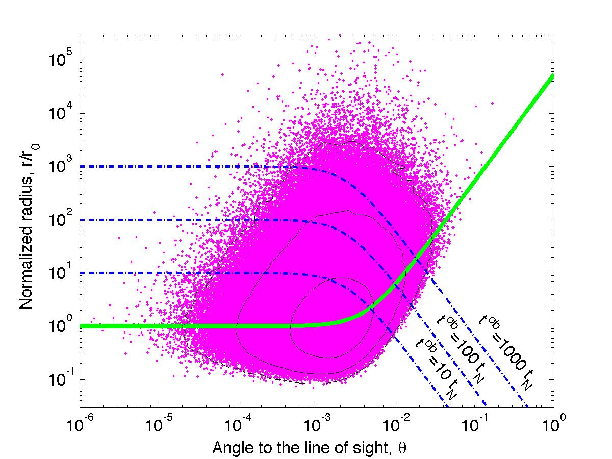
Figure 1.— Position of the last scattering event in $\theta$-$r$ plane for $10^{6.5}$ events. Parameters chosen in producing the plot are $L=10^{52}\rm{\,erg\,s^{-1}}$ and $\Gamma=400$. The solid (green) line is the photospheric radius, calculated in equation 3. Clearly, the last scattering events occur over a wide range of radii and angles. The photospheric radius gives only a first order approximation to the position of these events. The contour lines are added to the plot in order to indicate the density of the emerging photons radii and angles. The blue (dashed) lines are equal arrival time contours, calculated in equation 5. While at early times, $t\gtrsim t_{N}$ the emission is dominated by photons scattered at angles $\theta<\Gamma^{-1}$, at late times, photons emitted from large angles dominate the flux, a fact that gives rise to the flattening of the spectrum.

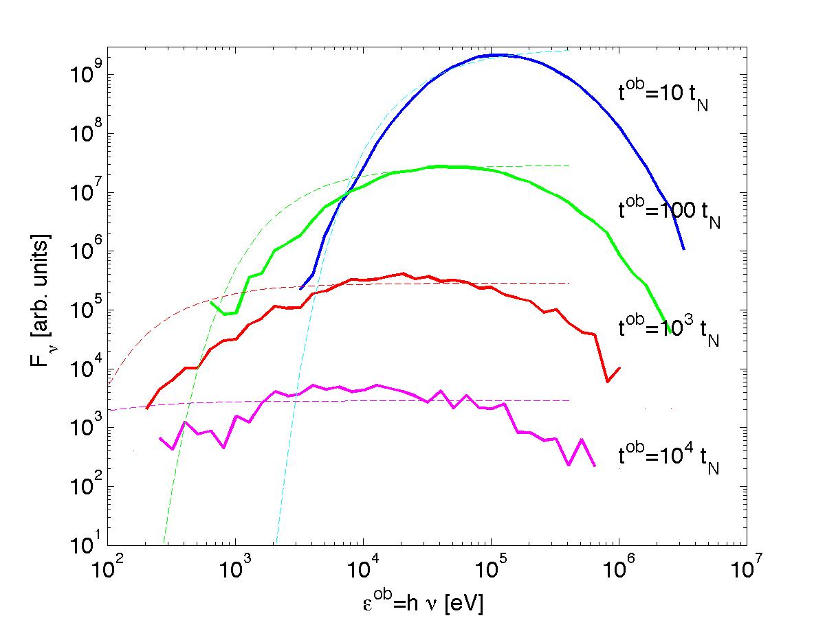
Figure 2.— Observed spectrum at different times, $t/t_{N}=10,10^{2},10^{3},10^{4}$. The solid lines are the results of the numerical simulation, and the dashed (thin) lines are the analytical approximation derived in equation 11. For initial expansion radius $r_{i}=10^{8}$ cm and other parameters same as in figure 1, as considered here, $T_{\max}^{ob}=430\rm{\,keV}$ (see text for further details). At late times, $t\gg t_{N}$, the spectrum becomes flat, $F_{\nu}\propto\nu^{0}$ over a wide spectral range below $T_{\max}^{ob}$. This spectrum is very different than the Rayleigh-Jeans tail of a thermal spectrum.

5. Summary and discussion

In this manuscript, we have studied both analytically and numerically the spectrum resulting from a photospheric emission in relativistically expanding plasma. We showed that even for purely thermal distribution of the comoving photon spectrum, aberration of the light results in an observed spectrum at late times that is very different from a Planck distribution. We showed that at late times, $t\gg t_{N}$, the observed spectrum approaches a power law, with power law index $F_{\nu}\propto\nu^{0}$ over a wide spectral range. This result is remarkably similar to the observed low energy spectral index of many GRBs (Preece et al. , 2000; Kaneko et al. , 2006, 2008).

The origin of this non-trivial result lies in two facts: First, at late times, the emission is dominated by photons emitted off-axis (from angles $\theta\gg\Gamma^{-1}$, see figure 1). Due to the strong dependence of the Doppler shift on the angle to the line of sight, these photons are seen at much lower energies than photons emitted on-axis. Second, at any given instance, an observer sees simultaneously photons that are emitted from a range of radii and angles (see eq. 5). As each photon has a finite probability of being emitted from a given radius, and is seen at a particular Doppler shift, the observed spectrum and flux can only be described in terms of probability density functions (see §3). These functions provide a mathematical tool to describe the probability of photons to be emitted from radius $r$ and into angle $\theta$. Using these functions, we calculated an analytical approximation to the observed spectrum (eq. 11), which is the main result of this work. The analytical approximation was tested with a Monte-Carlo simulation that tracks the evolution of thermal photons in relativistically expanding plasma (§4). The simplified analytical calculations are found to be in very good agreement with the accurate numerical results (see figure 2).

In spite of the success in reproducing the low energy spectral slopes at late times, the theory is still not completed. For parameters characterizing GRBs, the thermal peak ( $T_{\max}^{ob}$) naturally falls at the sub-MeV range (see §4.1), hence the observed peak can naturally be explained as having a thermal origin. However, a noticeable drawback of the theory as stated in this manuscript, is that the same parameters lead to very short characteristic time scale, $t_{N}\approx 10^{-5}$ s. Since above $t_{N}$ the flux decays rapidly, $F_{\nu}(t)\propto t^{-2}$ (see eq. 11), one expects a relatively weak thermal signal at $t\gg t_{N}$, which can still be very short time. We note though, that the calculation of $t_{N}$ in equation 5 is based on the assumption of constant outflow velocity. This assumption is too simplified: in order to reach high Lorentz factor, the plasma needs to undergo an acceleration phase, and so the average Lorentz factor below the photosphere is less than the terminal Lorentz factor. As a result, we expect that in practice the characteristic time scale relevant for thermal emission in GRBs is longer than the one considered in equation 5.

The exact delay time depends on several uncertain conditions. One is the content of the fireball: for example, Poynting-flux dominated fireball is expected to have slower acceleration than matter dominated fireball (Drenkhahn, 2002; Drenkhahn & Spruit, 2002; Giannios & Spruit, 2005, 2006). Another is the baryon load (Ioka, 2010), and in particular the baryon distribution along the jet (Morsony et al. , 2007; Lazzati et al. , 2009; Mizuta et al. , 2010): although in this manuscript we considered a steady outflow, clearly the outflow in GRBs is characterized by regions of higher and lower densities, and is thus not steady (edge effects due to the finite opening angle may also play a role at late times).

An additional source of discrepancy between the theoretical predictions developed in this paper and the observed spectrum, lies in the fact that the theory here does not consider any additional, non-thermal radiative processes. As shown here, photospheric emission is capable of reproducing the peak energy and the low energy spectral slope ($\alpha$ in the “Band” function) seen in GRBs (at late times). However, photospheric emission is not capable of of producing high energy photons (above $T_{\max}^{ob}\lesssim\rm{\,MeV}$), as are seen in some GRBs by the LAT detector on board the Fermi satellite. The inclusion of high energy, non-thermal photons, necessitates additional radiative mechanisms, that must take place following dissipation processes that occur above the photosphere (e.g., in GRB080916C analysis of the high energy emission imply Poynting dominated outflow; see Zhang & Pe’er, 2009). Additional radiative mechanisms, such as synchrotron emission or Compton scattering, naturally produce a broad band energy spectrum, and thus may contribute not only to the high energy spectrum but to the low energy part (below the thermal peak) as well. The overall observed spectra below the thermal peak is thus generally expected to be hybrid- i.e., composed of both thermal and non-thermal parts. The exact contribution of the non-thermal part may vary from burst to burst, depending on the values of the free model parameters, such as the radius of the photosphere, the dissipation radius, the strength of the magnetic field, etc.

In principle, the inclusion of thermal photons contributes to the high energy, non thermal part of the spectrum as well, as these photons serve as seed photons for Compton scattering by the non-thermal electrons and hot pairs (Rees & Mészáros, 2005; Pe’er et al. , 2005, 2006; Lazzati & Begelman, 2010; Beloborodov, 2010). The exact contribution of the thermal photons depend on the optical depth at the dissipation radius. If the dissipation radius is close to the photosphere, the resulting spectrum has a complex shape, that is very different than either a thermal spectrum or the optically thin synchrotron - synchrotron self Compton (SSC) model predictions (Pe’er et al. , 2005, 2006). On the other hand, if the dissipation occurs at large radii, the two components, thermal and non-thermal, can be decoupled, a fact that can lead to a clear identification of the thermal component, as is in the case of GRB090902B (Ryde et al. , 2010; Pe’er et al. , 2010).

One clear prediction of the results presented here, is that if a thermal component contributed significantly to the observed spectrum, than the low energy spectral slope ($\alpha$) is expected to vary with time: at early times, when the inner engine is active, $\alpha$ is expected to be steep (close to the Rayleigh-Jeans tail), while at later times, $F_{\nu}\propto\nu^{0}$. This result is expected to be correlated with a decay of the peak energy and the thermal flux, and was possibly observed in several bursts (e.g., Crider et al. , 1997; Ghirlanda et al. , 2007; Ryde & Pe’er, 2009; Page et al. , 2009). We note though that in many GRBs, the data is not easily compared to the theoretical prediction, since the outflows in GRBs are generally not smooth, but very fluctuative. Therefore, photons originating from different emission episodes (each characterized by its own mass loss ejection rate and its own Lorentz factor) are often superimposed. Thus, in fact, thermal photons may only be identified using detailed time resolved spectral analysis of separate flares. This task was carried by Ryde & Pe’er (2009), which were indeed able to identify the thermal component in a large sample of bursts. Once done, this analysis method can be further used to deduce the properties of the GRB outflow (Pe’er et al. , 2007).

In addition to the prompt emission phase in GRBs, thermal activity may occur as part of the flaring activity observed in the early afterglow phase of many GRBs (Burrows et al. , 2005; Falcone et al. , 2007; Chincarini et al. , 2010; Margutti et al. , 2010). The exact nature of these flares is currently not yet clear. As it is plausible that the flares result from renewed emission from the inner core, a renewed thermal emission may occur. The analysis presented here may therefore apply in the study of the late time flares as well.

While analysis of GRB prompt emission spectrum serves as a major motivation to this work, we note that the analysis presented here is general. With modified parameters values, the analysis apply to emission from any astronomical transient, which is characterized by relativistic outflow speeds and high density core. Thus, we expect the analysis carried here to be valid for objects such as AGNs and microquasars. This is valid because the exact nature of the radiative process that produces the thermal photons is of no importance, as long as the emission occurs deep enough in the flow, where the optical depth is high, $\tau\gg 1$.

References

- Abramowicz et al. (1991) Abramowicz M.A., Novikov, I.D., & Paczyński, B. 1991, ApJ, 369, 175
- Bellm (2010) Bellm, E. C. 2010, ApJ, 714, 881
- Beloborodov (2010) Beloborodov, A.M. 2010, MNRAS, in press (arXiv:0907:0732)
- Berger et al. (2003) Berger, E., Kulkarni, S.R., & Frail, D. 2003, ApJ, 590, 379
- Bos̆njak et al. (2009) Bos̆njak, Z., Daigne, F., & Dubus, G. 2009, A&A, 498, 677
- Burrows et al. (2005) Burrows, D.N., et al. 2005, Science, 309, 1833
- Chincarini et al. (2010) Chincarini, G., et al. 2010, MNRAS, 406, 2113
- Cohen et al. (1997) Cohen, E., et al. 1997, ApJ, 488, 330
- Crider et al. (1997) Crider, A., et al. 1997, ApJ, 479, L39
- Daigne & Mochkovitch (1998) Daigne, F., & Mochkovitch, R. 1998, MNRAS, 296, 275
- Daigne & Mochkovitch (2002) Daigne, F., & Mochkovitch, R. 2002, MNRAS, 336, 1271
- Dermer & Böttcher (2000) Dermer, C.D., & Böttcher, M. 2000, ApJ, 534, L155
- Drenkhahn (2002) Drenkhahn, G. 2002, A&A, 387, 714
- Drenkhahn & Spruit (2002) Drenkhahn, G., & Spruit, H. 2002, A&A, 391, 1141
- Eichler & Levinson (2000) Eichler, D., & Levinson, A. 2000, ApJ, 529, 146
- Falcone et al. (2007) Falcone, A.D., et al. 2007, ApJ, 671, 1921
- Ghirlanda et al. (2003) Ghirlanda, G., Celotti, A., & Ghisellini, G. 2003, A& A, 406, 879
- Ghirlanda et al. (2007) Ghirlanda, G., et al. 2007, MNRAS, 379, 73
- Giannios & Spruit (2005) Giannios, D., & Spruit, H. 2005, A&A, 430, 1
- Giannios & Spruit (2006) Giannios, D., & Spruit, H. 2006, A&A, 450, 887
- Goodman (1986) Goodman, J. 1986, ApJ, 308, L43
- Gopal-Krishna et al. (2006) Gopal-Krishna, et al. 2006, MNRAS, 377, 446
- Guetta et al. (2001) Guetta, D., Spada, M., & Waxman, E. 2001, ApJ, 557, 399
- Hjellming & Rupen (1995) Hjellming, R.M., & Rupen, M.P. 1995, Nature, 375, 464
- Ioka (2010) Ioka, K. 2010, preprint (arXiv:1006.3073)
- Kaneko et al. (2006) Kaneko, Y., et al. 2006, ApJS, 166, 298
- Kaneko et al. (2008) Kaneko, Y., et al. 2008, ApJ, 677, 1168
- Kobayashi et al. (1997) Kobayashi, S., Piran, T., & Sari, R. 1997, ApJ, 490, 92
- Lazzati & Begelman (2010) Lazzati, D., & Begelman, M.C. 2010, ApJ, submitted (arXiv:1005.4704)
- Lazzati et al. (1999) Lazzati, D., Ghisellini, G., & Celotti, A. 1999, ApJ, 523, L113
- Lazzati et al. (2009) Lazzati, D., Morsony, B.J., & Begelman, M.C. 2009, ApJ, 700, L47
- Lind & Blandford (1985) Lind, K.R., & Blandford, R.D. 1985, ApJ, 295, 358
- Margutti et al. (2010) Margutti, R., et al. 2010, MNRAS, 406, 2149
- Medvedev (2000) Medvedev, M.V. 2000, ApJ, 540, 704
- Mészáros (2006) Mészáros, P. 2006, Rep. Prog. Phys., 69, 2259
- Mészáros et al. (2002) Mészáros, P., Ramirez-Ruiz, E., Rees, M.J., & Zhang, B. 2002, ApJ, 578, 812
- Mészáros & Rees (2000) Mészáros, P., & Rees, M.J. 2000, ApJ, 530, 292
- Mirabel & Rodriguez (1994) Mirabel, I.F., & Rodriguez, L.F. 1994, Nature, 371, 46
- Mizuta et al. (2010) Mizuta, A., Nagataki, S., & Aoi, J. 2010, preprint (arXiv:1006.2440)
- Morsony et al. (2007) Morsony, B.J., Lazzati, D., & Begelman, M.C. 2007, ApJ, 665, 569
- Nysewander et al. (2009) Nysewander, M., Fruchter, A., & Pe’er, A. 2009, ApJ, 701, 824
- Paczyński (1986) Paczyński, B. 1986, ApJ, 308, L43
- Paczyński (1990) Paczyński, B. 1990, ApJ, 363, 218
- Page et al. (2009) Page, K.L. et al. 2009, MNRAS, 400, 134
- Panaitescu et al. (1999) Panaitescu, A., Spada, M., & Mészáros, P. 1999, ApJ, 522, L105
- Pe’er (2008) Pe’er, A. 2008, ApJ, 682, 463
- Pe’er et al. (2005) Pe’er, A., Mészáros, P., & Rees, M.J. 2005, ApJ, 635, 476
- Pe’er et al. (2006) Pe’er, A., Mészáros, P., & Rees, M.J. 2006, ApJ, 642, 995
- Pe’er et al. (2006b) Pe’er, A., Mészáros, P., & Rees, M.J. 2006, ApJ, 652, 482
- Pe’er et al. (2007) Pe’er, A., Ryde, F., Wijers, R.A.M.J., Mészáros, P., & Rees, M.J. 2007, ApJ, 664, L1
- Pe’er & Waxman (2004) Pe’er, A., & Waxman, E. 2004, ApJ, 613, 448
- Pe’er & Zhang (2006) Pe’er, A., & Zhang, B. 2006, ApJ, 653, 454
- Pe’er et al. (2010) Pe’er, A., et al. 2010, ApJ, submitted (arXiv:1007.2228)
- Piran (2005) Piran, T. 2005, Rev. Mod. Phys. 76, 1143
- Preece et al. (1998) Preece, R.D., et al. 1998, ApJ, 506, L23
- Preece et al. (2000) Preece, R.D., et al. 2000, ApJS, 126, 19
- Preece et al. (2002) Preece, R.D., et al. 2002, ApJ, 581, 1248
- Rees & Mészáros (1994) Rees, M.J., & Mészáros, P. 1994, ApJ, 430, L93
- Rees & Mészáros (2005) Rees, M.J., & Mészáros, P. 2005, ApJ, 628, 847
- Ryde (2004) Ryde, F. 2004, ApJ, 614, 827
- Ryde (2005) Ryde, F. 2005, ApJ, 625, L95
- Ryde & Pe’er (2009) Ryde, F., & Pe’er, A. 2009, ApJ, 702, 1211
- Ryde et al. (2010) Ryde, F., et al. 2010, ApJ, 709, L172
- Sari & Piran (1997) Sari, R., & Piran, T. 1997, MNRAS, 287, 110
- Tavani (1996) Tavani, M. 1996, ApJ, 466, 768
- Zhang & Pe’er (2009) Zhang, B., & Pe’er, A. 2009, ApJ, 700, L65
- Zhang et al. (2007) Zhang, B., et al. 2007, ApJ, 655, 989