Escaping stars from young low-$N$ clusters

Abstract

With the use of $N$-body calculations the amount and properties of escaping stars from low-$N$ ($N$ = 100 and 1000) young embedded star clusters prior to gas expulsion are studied over the first 5 Myr of their existence. Besides the number of stars also different initial radii and binary populations are examined as well as virialised and collapsing clusters. It is found that these clusters can loose substantial amounts (up to 20%) of stars within 5 Myr with considerable velocities up to more than 100 km/s. Even with their mean velocities between 2 and 8 km/s these stars will still be travelling between 2 and 30 pc during the 5 Myr. Therefore can large amounts of distributed stars in star-forming regions not necessarily be counted as evidence for the isolated formation of stars.

1 Introduction

Stars do not form in absolute isolation but rather in groups or embedded clusters in dense molecular cloud cores (Lada & Lada, 1995, 2003; Adams & Myers, 2001; Allen et al., 2007). Theoretical and observational results indicate that these groups and the majority of the embedded clusters dissolve quickly due to gas expulsion after about 10 Myr and release their stars into the galactic field (Kroupa et al., 2001; Kroupa & Bouvier, 2003; Adams & Myers, 2001; Lada & Lada, 2003; Weidner et al., 2007; Baumgardt & Kroupa, 2007). But the ratio of the distributed mode of star formation and the clustered one is not fully understood. Observations show a distributed fraction of stars in the Orion molecular clouds of about 20% (Allen et al., 2007). It is generally assumed that these fraction is primordial as dynamical evolution of the clusters is considered to slow to reproduce the observed fraction of isolated stars at such a young stage. But for a full physical understanding of the formation of stars it is vital to know all modes of star formation in as much detail as possible. The purpose of this work is therefore to access whether or not the observed amount of distributed stars outside embedded clusters could have a dynamical origin and henceforth being initially formed in the young, tight embedded clusters or if there is intrinsically isolated star formation. Especially in star-forming regions which do not show massive star clusters the amount of stars released through the dynamical evolution of low-$N$ clusters is not well known. In order to study this question a large series of $N$-body calculations is performed and the number, the velocity and the mass spectrum of stars ejected due to dynamical interactions within 5 Myrs from this clusters are studied.

2 The cluster setup

With the use of the $N$-body6 code (Aarseth, 1999a, b, 2003, 2008) the evolution of numerical star clusters with small numbers of stars are examined. Two different numbers of stars, $N$, are used, 100 and 1000. As the actual number of escaped stars can be rather low each set of initial conditions is simulated 100 times using different random number seeds to set up the masses, velocities and positions of the stars in order to improve the statistical significance of the results. All stars in the clusters follow the canonical IMF (Kroupa, 2002).

Besides the initial number of stars several other initial parameters are studied with each 100 calculations.

• All stars are initially single stars,

• all stars reside in binaries,

• 50% of the stars are in binaries,

• the cluster is initially in virial equilibrium ,

• the cluster is initially sub-virial (collapsing with the kinetical energy being one-tenth of the potential energy).

• All star clusters are setup as Plummer-spheres (Plummer, 1911) with different initial half-mass radii of 0.1, 0.25 or 0.5 pc.

Each of these setups are then numerically evolved with $N$-body6 for 5 Myr. The evolution time of 5 Myr is chosen to minimise mass loss due to stellar evolution, to avoid supernovae and primarily to have a setting of a star cluster still embedded in its parental cloud, prior to gas expulsion. Though, clusters initially probably form from clumpy structures (Williams et al., 2000; Carpenter & Hodapp, 2008). Simulations of sub-virial clumpy initial conditions (Allison et al., 2009) have shown that such clusters mass segregate faster than virial clusters due to the formation of short-lived very dense cores. But these calculations did not include a background gas potential.

To emulate the gas in which the stars are embedded during this time, the cluster is setup with an additional plummer potential (Plummer, 1911; Binney & Tremaine, 1987) of the same half-mass radius and the same mass as the cluster. Thus assuming a star-formation efficiency (SFE) of 50%. Though, global SFE’s are observationally around 30% (Lada & Lada, 2003), locally within the region where the cluster actually forms the value is most likely higher (Moeckel & Bate, 2010). A SFE of 50% has therefore been chosen. A large differences in results between 30 and 50% SFE is not to be expected. The gas potential is in all cases kept constant during the whole calculation time. As the results are qualitatively similar to $N$-body studies without a gas background potential (e.g. Kroupa, 1998; Kroupa & Bouvier, 2003), the exact shape of the potential does not seems to be overly important. But detailed further studies are needed to clarify the full impact of the shape and depth of the potential on the properties of escaping stars.

The decision to include primordial binaries into the study is based on the observational results that open clusters host large number of binaries (Sana et al., 2009; Sollima et al., 2010). The initial setup of the binary properties increase the total parameter space of the calculations significantly. As a cluster of the richness of the Orion Nebula cluster stellar dynamics may change the mass function and binary properties in the core significantly in less than $10^{6}$ yr (Goodwin & Bastian, 2006; Pflamm-Altenburg & Kroupa, 2006; Pfalzner & Olczak, 2007; Allison et al., 2009). And as the majority of the present-day field binaries are being processed through star clusters, their properties are not suited to be used for the numerical setup (Duquennoy & Mayor, 1991; Kroupa, 1995a, d, b, c; Kroupa & Bouvier, 2003). Therefore, the results of the inverse dynamical population synthesis of Kroupa (1995b) are used, which predict a flat (thermal) period distribution (resulting in a uniform logarithmic semi-major axis distribution) and random pairing of the stars in systems of low-mass ($<$ 1 $M_{\odot}$) stars (Kroupa, 1995b, c). While there are indications for non-random pairing of massive stars (Kobulnicky & Fryer, 2007; Weidner et al., 2009), the low-mass results are also used for massive binaries in this study. Firstly, because the mass where a change of properties might occur is not determined yet and it is not clear if mass-ratios near to unity for massive stars are primordial or already a sign of dynamical evolution (Pfalzner & Olczak, 2007) and secondly, because due to the choice of $N$ = 100 and 1000, only a relatively small number of massive stars is to be expected anyway. For example, there should be only three stars above 8 $M_{\odot}$ for $N$ = 1000 and a Kroupa-IMF.

It should be noted here, that rapid changes in the binary properties might also at least partly due to the initial conditions of $N$-body calculations and do not really reflect the star formation process. I.e. that unstable binaries that are easily destroyed in early cluster dynamics may not even form in the first place (Moeckel & Bate, 2010).

In the $N$ = 1000 cases, for the IMF a maximal mass, $m_{\mathrm{max}}$, of 25 $M_{\odot}$ is chosen, in accordance with the $m_{\mathrm{max}}-M_{\mathrm{ecl}}$-relation by Weidner et al. (2010). In the $N$ = 100 case this relation yields a $m_{\mathrm{max}}$ of 7 $M_{\odot}$. But also comparison calculations are done using $m_{\mathrm{max}}$ = 25 $M_{\odot}$ for the $N$ = 100 case.

3 Results

In the series of Figs. 1 to 8 the results of the $N$-body6 calculations after 5 Myr are presented. There the mean number of lost stars, $<$$N_{\mathrm{lost}}$$>$, the mean lost fraction of mass, $<$$M_{\mathrm{lost}}$$>$/$<$$M_{\mathrm{tot}}$$>$, the mean escape velocity, $<$$v_{\mathrm{esc}}$$>$, the mean escape velocity dispersion, $<$$\sigma$$>$, and the mean mass of the lost stars, $<$$m_{\mathrm{lost}}$$>$, are studied in dependence of the initial cluster relaxation time, $t_{\mathrm{relax}}$. The latter is calculated by using the following equations from Binney & Tremaine (1987):

$$t_{\mathrm{relax}}\approx\frac{N}{8\ln{N}}t_{\mathrm{cross}},$$ (1)

with $N$ being the number of stars and $t_{\mathrm{cross}}$ the crossing time a star needs to travel through the cluster which is given by,

$$t_{\mathrm{cross}}=2\sqrt{\frac{R_{\mathrm{ecl}}^{3}}{GM_{\mathrm{tot}}}},$$ (2)

with $G$ being Newton’s gravitational constant, $R_{\mathrm{ecl}}$ the cluster radius and $M_{\mathrm{tot}}$ its mass.

It is important to note that the relaxation time of a cluster is not a constant but also evolves with time. Though, for the clusters which start in virial equilibrium, the change is negligible over the short period of time studied here. The clusters expand about $\sim$10% due to evolutionary and dynamical mass loss. This leads to a $\sim$10% increase in $t_{\mathrm{relax}}$. But as the sub-virial clusters contract significantly during the calculation time span, their $t_{\mathrm{relax}}$ decreases and becomes comparable to a cluster with half their half-mass radius.

In the B panels of the Figs. 3 and 7 are additionally shown several literature descriptions of star loss. The first one is the analytical description of Binney & Tremaine (1987, Eq. 8-85) based on the Fokker-Planck approximation for the mass loss by evaporation of stars from a cluster (with large $N$).

$$M(t)=M_{0}\left(1-\frac{7k_{\mathrm{e}}t}{2t_{\mathrm{relax}}^{0}}\right)^{2/7},$$ (3)

with $M_{0}$ being the initial cluster mass, $k_{\mathrm{e}}$ $\approx$ 0.003 and $t_{\mathrm{relax}}^{0}$ the initial relaxation time (eq. 1). With the use of the mean mass, $m_{\mathrm{mean}}$ of the IMF, which is for a Kroupa IMF $m_{\mathrm{mean}}$ $\approx$ 0.36 $M_{\odot}$, the number of stars lost over time can be approximated:

$$N(t)=M(t)/m_{\mathrm{mean}}.$$ (4)

This equation is indicated with solid black dots in the two Figs. 3 and 7.

This description is strictly valid only for large $N$ and does not seem to provide a good characterisation of the $N$-body calculations. Heggie (1974) assumed that in low-$N$ clusters binary interactions should dominate over the evaporation of stars. He formulated the following dissolution time scale for low-$N$ clusters:

$$t_{\mathrm{diss}}=\frac{N^{2}}{100}t_{\mathrm{cross}},$$ (5)

which can also be used to estimate the star loss from a cluster in the following way:

$$N_{\mathrm{diss}}=N_{0}e^{-\frac{\ln(N_{0})}{t_{\mathrm{diss}}}t},$$ (6)

were $N_{0}$ is the initial number of stars. This description is included as open squares in the Figs. 3 and 7.

An third description of stellar loss can be derived from the evaporation time scale when assuming the collisionless Boltzmann equation given in Binney & Tremaine (1987).

$$t_{\mathrm{evap}}=136t_{\mathrm{relax}},$$ (7)

which can be transformed into the following number loss formula:

$$N_{\mathrm{evap}}=N_{0}e^{-\frac{\ln(N_{0})}{t_{\mathrm{evap}}}t},$$ (8)

where $N_{0}$ is the initial number of stars. In the Figs. 3 and 7 this relation is plotted as open triangles.

The Figs. 1 to 4 show the results using the star clusters with initially $N$ = 1000 after 5 Myr while the Figs. 5 to 8 show the same for $N$ = 100.

Figure 1: Mean number of stars lost vs $t_{\mathrm{relax}}$ (Panel A) and mean percentage of cluster mass lost vs $t_{\mathrm{relax}}$ (Panel B). The solid line shows the case without any initial binaries, the dotted line is the 50% initial binary case, the dashed line is the 100% initial binaries case and the dashed-dotted line marks the sub-virial case.

Figure 2: Mean escape velocity, $<$$v_{\mathrm{esc}}$$>$, vs $t_{\mathrm{relax}}$ (Panel A) and mean velocity dispersion, $<$$\sigma$$>$, vs $t_{\mathrm{relax}}$ (Panel B). The solid line shows the case without any initial binaries, the dotted line is the 50% initial binary case, the dashed line is the 100% initial binaries case and the dashed-dotted line marks the sub-virial case.

Figure 3: Panel A: Mean mass of the escaped stars vs $t_{\mathrm{relax}}$. The solid line shows the case without any initial binaries, the dotted line is the 50% initial binary case, the dashed line is the 100% initial binaries case and the dashed-dotted line marks the sub-virial case. Panel B: Total number of lost stars vs number of relaxation times the cluster experienced during the 5 Myr simulation time. The solid line shows the case without any initial binaries, the dotted line is the 50% initial binary case, the dashed line is the 100% initial binaries case and the dashed-dotted line marks the sub-virial case. The solid black dots are the predicted numbers from eq. 4, the open squares from eq. 6 and the open triangles from eq. 8.

Figure 4: Median and maximal flight ranges from the cluster centre of the escaped stars vs $t_{\mathrm{relax}}$. The solid line shows the case without any initial binaries, the dotted line is the 50% initial binary case, the dashed line is the 100% initial binaries case and the dashed-dotted line marks the sub-virial case.

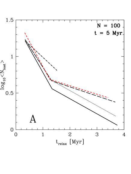
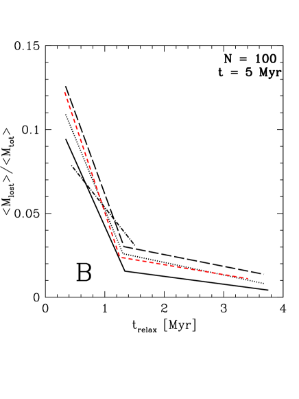
Figure 5: Mean number of stars lost vs $t_{\mathrm{relax}}$ (Panel A) and mean percentage of cluster mass lost vs $t_{\mathrm{relax}}$ (Panel B). The solid line shows the case without any initial binaries, the dotted line is the 50% initial binary case, the long-dashed line is the 100% initial binaries case, the dashed-dotted line marks the sub-virial case and short-dashed line the case with $m_{\mathrm{max}}$ = 25 $M_{\odot}$.

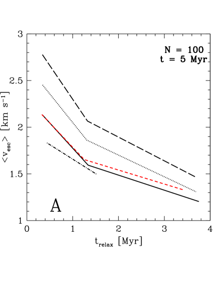
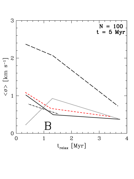
Figure 6: mean escape velocity vs $t_{\mathrm{relax}}$ (Panel A) and mean velocity dispersion vs $t_{\mathrm{relax}}$ (Panel B). The solid line shows the case without any initial binaries, the dotted line is the 50% initial binary case, the long-dashed line is the 100% initial binaries case, the dashed-dotted line marks the sub-virial case and short-dashed line the case with $m_{\mathrm{max}}$ = 25 $M_{\odot}$.

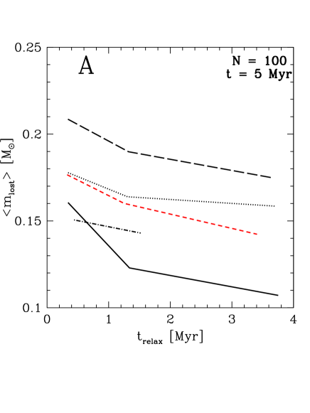
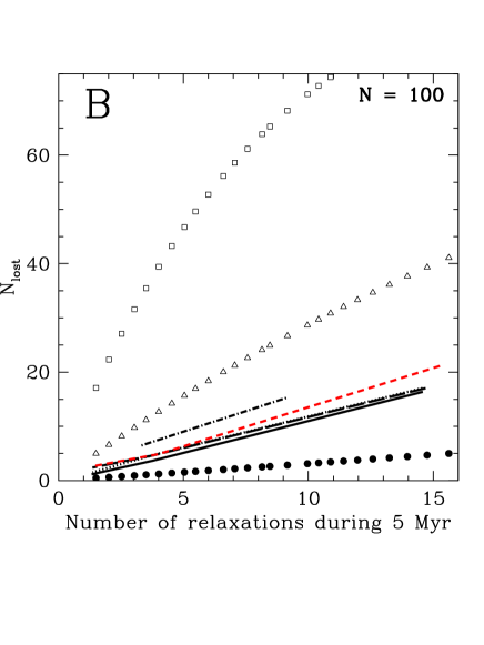
Figure 7: Panel A: Mean mass of the escaped stars vs $t_{\mathrm{relax}}$. The solid line shows the case without any initial binaries, the dotted line is the 50% initial binary case, the long-dashed line is the 100% initial binaries case, the dashed-dotted line marks the sub-virial case and short-dashed line the case with $m_{\mathrm{max}}$ = 25 $M_{\odot}$. Panel B: Total number of lost stars vs number of relaxation times the cluster experienced during the 5 Myr simulation time. The solid line shows the case without any initial binaries, the dotted line is the 50% initial binary case, the long-dashed line is the 100% initial binaries case, the dashed-dotted line marks the sub-virial case and short-dashed line the case with $m_{\mathrm{max}}$ = 25 $M_{\odot}$. The solid black dots are the predicted numbers from eq. 4, the open squares from eq. 6 and the open triangles from eq. 8.

Figure 8: Median and maximal flight ranges from the cluster centre of the escaped stars vs $t_{\mathrm{relax}}$. The solid line shows the case without any initial binaries, the dotted line is the 50% initial binary case, the dashed line is the 100% initial binaries case, the dashed-dotted line marks the sub-virial case and short-dashed line the case with $m_{\mathrm{max}}$ = 25 $M_{\odot}$.

4 Discussion

As is visible in Fig. 1, the number and mass fraction of lost stars for the N=1000 clusters is only dependent on the initial radius of the cluster ($\rightarrow$ $t_{\mathrm{relax}}$), while the binary fraction does not play a major role. Likewise in the case of a collapsing cluster (sub-virial, dashed-dotted line). A sub-virial cluster just behaves like a somewhat more concentrated cluster as they collapse and therefore change their timescales.

In the case of the $N$ = 100 clusters (Fig. 5) there seems to be a dependence of the number loss on the binary fraction for objects with large radii ($t_{\mathrm{relax}}$ $>$ 2 Myr). But this might still be a low-number stochastic effect as only a couple of stars leave these clusters ($N_{\mathrm{lost}}$ $<$ 5). When comparing the lost mass fraction of the $N$ = 1000 and $N$ = 100 calculations, the richer cluster seem to loose 2 or 3% more mass, reflecting the higher encounter rate in the richer objects. Allowing for more massive stars in the low-$N$ clusters (short-dashed lines in Figs. 5 to 7) increases the star loss by similar amounts as a high-binary fraction. This is probably due to the higher average mass of the systems compared to single stars. A higher upper mass limit of the IMF likewise increases the average stellar mass. A larger average mass leads to higher momenta and therefore to larger velocities after 2- and 3-body interactions which are then more likely to exceed the escape velocity of the cluster.

Like the mass loss, the mean escape velocity, $<$$v_{\mathrm{esc}}$$>$ (Panel A of Fig. 2), is mainly depended on $t_{\mathrm{relax}}$, though the existence of a high-binary fraction raises $<$$v_{\mathrm{esc}}$$>$ by about 1 km/s, independent of $t_{\mathrm{relax}}$. Primordial binaries introduce 3- and 4-body interactions early-on in the cluster evolution opposed to the mainly 2-body interactions for single star-only clusters. Such higher order interactions generally result in larger velocities.

The mean velocity of the ejected stars in the case of $N$ = 1000 is 4 to 8 km/s (Fig. 2) and the escaped stars travel on the average up to 10 to 30 pc (Fig. 4) within 5 Myr depended on the original size of the cluster. But individual stars can be up to 1 kpc away, as the highest escape velocity encountered for the $N$ = 1000 clusters was about 260 km/s, though the typical range of escape velocities is between 2 and 40 km/s. These values are in the same range as the results of Kroupa (1998) who studied clusters with $N$ = 400 in a Galactic tidal field but without a gas background potential. A comparison with observations seem to contradict the relatively large number of lost stars found here. Tobin et al. (2009) study the surroundings of the Orion Nebula cluster (ONC) and find that the majority of stars with velocities differences to the cluster larger than 10 km/s have little or no IR-excess and are therefore most likely old and not associated with the ONC. When looking only at escapees with velocities larger than 10 km/s after only 1 Myr (the age of the ONC, Hillenbrand & Hartmann, 1998), only between 0 and 14 are to be expected from the $N$-body calculations, depending on the initial conditions. Interestingly, Tobin et al. (2009) do find 6 stars with a velocity offset above 10 km/s which have an IR-excess consistent of being young stars and therefore could have been ejected from the ONC, consistent with our predictions. As the Tobin et al. (2009) study can not differentiate between bound and unbound cluster stars below 10 km/s it is currently not possible to test the predictions of the $N$-body calculations further. Also consistent with this picture is the recently discovered halo of low-mass stars around the small young cluster $\eta$ Chamaeleontis (Murphy et al., 2010). Generally, though, is an IR-excess probably not a good age indicator for ejected stars as most of these had a close encounter with another star which lead to the ejection. During this encounter any disc around that star could be truncated or largely stripped, therefore reducing or eliminating the IR-excess. In order to search for a distributed population of ejected young stars around clusters the position of the stars in the HR diagram will likely be a more robust age indicator.

For less rich clusters (Panel A of Fig. 6), smaller $<$$v_{\mathrm{esc}}$$>$ are generally achieved. These are also increased by the presence of binaries by 0.5 to 1 km/s. Stars escaping from $N$ = 100 clusters on the average travel 3 to 6 pc (Fig. 8) within 5 Myr with a typical range of escape velocities between 1 and 12 km/s. For the low-$N$ clusters the fastest escaper had about 40 km/s and travelled about 100 pc in total. Interestingly, the mean of the velocity dispersion of escape velocities, $\sigma$, is more strongly affected by the presence of binaries, both in the $N$ = 1000 (Panel B of Fig. 2) and $N$ = 100 case (Panel B of Fig. 6). Therefore, the presence of large fractions of binaries, while only slightly enlarging the mean escape velocity, adds more scatter to the velocities of the escaping stars. This increases the area around a young embedded cluster where to expect escaping stars significantly by 50 to 200%. The mean mass of the escaping stars, however, seems to be rather independent of binaries in the $N$ = 1000 clusters but is strongly correlated with $t_{\mathrm{relax}}$ (Panel A of Fig. 3). It rises from about 0.22 $M_{\odot}$ in the 10 Myr case ($\rightarrow$ $R_{\mathrm{ecl}}$ = 0.5 pc) to about 0.4 $M_{\odot}$ for very compact (1 Myr $\rightarrow$ $R_{\mathrm{ecl}}$ = 0.1 pc) clusters, while for the collapsing clusters it stays at about 0.3 $M_{\odot}$. On the contrary for the low-$N$ = 100 clusters, $<$$m_{\mathrm{lost}}$$>$ roughly stays constant with $t_{\mathrm{relax}}$ (Panel A of Fig. 7) but varies strongly with the binary fraction. Here the sub-virial, 50% binary and higher upper mass limit case are rather similar and well separated from the only-single star case and the 100% binaries.

In appendix A histograms of the mass and $<$$v_{\mathrm{esc}}$$>$ of the escaped stars for the different initial conditions are shown. Mass histograms are only plotted for the cases without initial binaries for $N$ = 1000 and $N$ = 100 (Panels A of Figs. 9 and 10). The mass histograms in the $N$ = 1000 look very similar to the input IMF and for $N$ = 100 suffer from the low number of escaped stars. Velocity histograms are only shown for the cases with 100% initial binaries. All velocity histograms are also rather similar but the cases with binaries have a larger high-velocity tail when compared to the single star only run.

4.1 Comparison with analytical estimates

The Panels B of Figs. 3 and 7 show the number of stars lost per number of relaxations the clusters experiences during 5 Myr for $N$ = 1000 and $N$ = 100, respectively. Besides the results from the different initial conditions there are also shown the analytic estimates as given by eqs. 4 (solid black dots), 6 (open squares) and 8 (open triangles). In both cases the eq. 4 predicts far too low escape numbers which is expected as this equation should be applied only to clusters with large $N$. For the $N$ = 1000 case the resulting star loss is between the predictions of eqs. 6 and 8 but somewhat closer to the binary interaction dominated model (eq. 6). This can be seen as an indication that star-loss in such clusters is not purely dominated by binary interactions (eq. 6) but evaporation (eq. 8) already plays a role. Though, the pure evaporation model of eq. 8 technically also only applies to clusters with larger $N$. The sub-virial models are much higher above the predictions of eq. 6, probably because the shorter the time scales of the collapsing clusters lead to more binary interactions compared to the virial cases.

The lower $N$ clusters with $N$ = 100 behave different in the sense that the numerical number of escapees is in between the estimates given by eqs. 4 and 8, but the binary interaction dominated model (eq. 6) overestimates star-loss strongly, while the evaporation model (eq. 8) seems to give a result closer to the numerical calculations. Here it might be that higher escape velocity due to the background potential impedes the loss of stars after low-energy encounters. As the radii for the $N$ = 100 and the $N$ = 1000 clusters are the same, the more massive clusters have higher densities and therefore higher encounter rates. For these it is therefore more likely that they experience high-energy encounters compared to the $N$ = 100 clusters and therefore the $N$ = 1000 clusters might be less affected by the background potential.

It should be noted here that none of the analytical estimates take any background potential into account and only focus on one physical process for star-loss, either energy equipartition or binary interactions.

5 Conclusions

• Low-mass star clusters loose between 1% and 20% of their stars (between 1% and 15% of their mass) within their first 5 Myr.

• This is nearly independent whether or not the clusters have primordial binaries but collapsing clusters loose more stars.

• The mean velocities of the escaping stars depend on the richness of the cluster and its radius and can be up to 8.5 km/s for $N$ = 1000 and $R_{\mathrm{ecl}}$ = 0.1 pc. This is slightly enlarged if primordial binaries are present.

• The velocity dispersion of the escape velocities is about half of the mean escape velocity when less than 50% of the stars are in primordial binaries. In the case of high binary fractions it can be as large as the mean escape velocity itself.

• The mean mass of the escapees depends on the richness of the cluster, its radius and the presence of binaries and vary up to an factor of 4.

• None of the analytic estimates from the literature describe the star loss precisely but they generally give the right order of magnitude of lost stars.

• The currently known number of fast escapees in the ONC is consistent with the predictions of the $N$-body calculations.

Henceforth, as the majority of the escapees are not fast run-away stars but evaporate relatively slow, the presence of 10% to 20% of distributed stars in a young star-forming region can be attributed to dynamical ejections from low-$N$ embedded star clusters. Especially, when taking into account that un-resolved binaries and chance superpositions of stars will tend to underestimate the number of stars within a cluster (Kouwenhoven & de Grijs, 2008; Maíz Apellániz, 2008, 2009; Weidner et al., 2009). No such miscounting due to crowding is to be expected outside of the clusters, leading to a overestimation of the ratio of stars around clusters to stars inside of them. Current estimates for the amount of distributed stars in young star-forming regions are therefore not in contradiction with the assumptions that most stars are formed in tight embedded clusters, which is consistent with other $N$-body studies (Kroupa, 1998; Kroupa & Bouvier, 2003).

Appendix A Mass and velocity histograms

In this appendix are shown the histograms of the mass and velocities of the escaped stars. Fig. 9 shows a mass histogram and velocity histogram example for $N$ = 1000 while Fig. 10 shows the same histograms for $N$ = 100.

Figure 9: The mass function (Panel A) of the lost stars for the models started without initial binaries and with a 1000 stars. Panel B: velocity histogram for the case with 100% initial binaries. All models started without initial binaries and 1000 stars. The solid histogram is the $R_{\mathrm{ecl}}$ = 0.1 pc model, the dotted histogram is the $R_{\mathrm{ecl}}$ = 0.2 pc model, the short-dashed histogram is the $R_{\mathrm{ecl}}$ = 0.3 pc model, the long-dashed histogram is the $R_{\mathrm{ecl}}$ = 0.4 pc model and the dashed-dotted histogram is the $R_{\mathrm{ecl}}$ = 0.5 pc model. The solid line in the mass function histogram is the input IMF (not to scale).

Figure 10: The mass function (Panel A) of the lost stars for the models started without initial binaries and with a 100 stars. Panel B: velocity histogram for the case with 100% initial binaries. All The solid histogram is the $R_{\mathrm{ecl}}$ = 0.1 pc model, the dotted histogram is the $R_{\mathrm{ecl}}$ = 0.25 pc model and the long-dashed histogram is the $R_{\mathrm{ecl}}$ = 0.5 pc model. The solid line in the mass function histogram is the input IMF (not to scale).

References

- Aarseth (1999a) Aarseth, S. J. 1999a, PASP, 111, 1333
- Aarseth (1999b) Aarseth, S. J. 1999b, Celestial Mechanics and Dynamical Astronomy, 73, 127
- Aarseth (2003) Aarseth, S. J. 2003, Gravitational N-Body Simulations, ed. S. J. Aarseth
- Aarseth (2008) Aarseth, S. J. 2008, in Lecture Notes in Physics, Berlin Springer Verlag, Vol. 760, Lecture Notes in Physics, Berlin Springer Verlag, ed. S. J. Aarseth, C. A. Tout, & R. A. Mardling, 1–4020
- Adams & Myers (2001) Adams, F. C. & Myers, P. C. 2001, ApJ, 553, 744
- Allen et al. (2007) Allen, L., Megeath, S. T., Gutermuth, R., et al. 2007, in Protostars and Planets V, ed. B. Reipurth, D. Jewitt, & K. Keil, 361–376
- Allison et al. (2009) Allison, R. J., Goodwin, S. P., Parker, R. J., de Grijs, R., Portegies Zwart, S. F., & Kouwenhoven, M. B. N. 2009, ApJ, 700, L99
- Baumgardt & Kroupa (2007) Baumgardt, H. & Kroupa, P. 2007, MNRAS, 380, 1589
- Binney & Tremaine (1987) Binney, J. & Tremaine, S. 1987, Galactic dynamics (Princeton, NJ, Princeton University Press, 1987, 747 p.)
- Carpenter & Hodapp (2008) Carpenter, J. M. & Hodapp, K. W. 2008, The Monoceros R2 Molecular Cloud, ed. Reipurth, B., 899–+
- Duquennoy & Mayor (1991) Duquennoy, A. & Mayor, M. 1991, A&A, 248, 485
- Goodwin & Bastian (2006) Goodwin, S. P. & Bastian, N. 2006, MNRAS, 373, 752
- Heggie (1974) Heggie, D. C. 1974, in IAU Symposium, Vol. 62, Stability of the Solar System and of Small Stellar Systems, ed. Y. Kozai, 225–229
- Hillenbrand & Hartmann (1998) Hillenbrand, L. A. & Hartmann, L. W. 1998, ApJ, 492, 540
- Kobulnicky & Fryer (2007) Kobulnicky, H. A. & Fryer, C. L. 2007, ApJ, 670, 747
- Kouwenhoven & de Grijs (2008) Kouwenhoven, M. B. N. & de Grijs, R. 2008, A&A, 480, 103
- Kroupa (1995a) Kroupa, P. 1995a, ApJ, 453, 350
- Kroupa (1995b) Kroupa, P. 1995b, MNRAS, 277, 1491
- Kroupa (1995c) Kroupa, P. 1995c, MNRAS, 277, 1507
- Kroupa (1995d) Kroupa, P. 1995d, ApJ, 453, 358
- Kroupa (1998) Kroupa, P. 1998, MNRAS, 298, 231
- Kroupa (2002) Kroupa, P. 2002, Science, 295, 82
- Kroupa et al. (2001) Kroupa, P., Aarseth, S., & Hurley, J. 2001, MNRAS, 321, 699
- Kroupa & Bouvier (2003) Kroupa, P. & Bouvier, J. 2003, MNRAS, 346, 343
- Lada & Lada (2003) Lada, C. J. & Lada, E. A. 2003, ARA&A, 41, 57
- Lada & Lada (1995) Lada, E. A. & Lada, C. J. 1995, AJ, 109, 1682
- Maíz Apellániz (2008) Maíz Apellániz, J. 2008, ApJ, 677, 1278
- Maíz Apellániz (2009) Maíz Apellániz, J. 2009, ApJ, 699, 1938
- Moeckel & Bate (2010) Moeckel, N. & Bate, M. R. 2010, MNRAS, 404, 721
- Murphy et al. (2010) Murphy, S. J., Lawson, W. A., & Bessell, M. S. 2010, MNRAS, 406, L50
- Pfalzner & Olczak (2007) Pfalzner, S. & Olczak, C. 2007, A&A, 475, 875
- Pflamm-Altenburg & Kroupa (2006) Pflamm-Altenburg, J. & Kroupa, P. 2006, MNRAS, 373, 295
- Plummer (1911) Plummer, H. C. 1911, MNRAS, 71, 460
- Sana et al. (2009) Sana, H., Gosset, E., & Evans, C. J. 2009, MNRAS, 400, 1479
- Sollima et al. (2010) Sollima, A., Carballo-Bello, J. A., Beccari, G., Ferraro, F. R., Pecci, F. F., & Lanzoni, B. 2010, MNRAS, 401, 577
- Tobin et al. (2009) Tobin, J. J., Hartmann, L., Furesz, G., Mateo, M., & Megeath, S. T. 2009, ApJ, 697, 1103
- Weidner et al. (2010) Weidner, C., Kroupa, P., & Bonnell, I. A. 2010, MNRAS, 401, 275
- Weidner et al. (2009) Weidner, C., Kroupa, P., & Maschberger, T. 2009, MNRAS, 393, 663
- Weidner et al. (2007) Weidner, C., Kroupa, P., Nürnberger, D. E. A., & Sterzik, M. F. 2007, MNRAS, 376, 1879
- Williams et al. (2000) Williams, J. P., Blitz, L., & McKee, C. F. 2000, Protostars and Planets IV, 97