Revised Supernova Rates from the IfA Deep Survey

Abstract

The IfA Deep survey uncovered $\sim$130 thermonuclear supernovae (TN SNe, i.e. Type Ia) candidates at redshifts from $z=0.1$ out to beyond $z=1$. The TN SN explosion rates derived from these data have been controversial, conflicting with evidence emerging from other surveys. This work revisits the IfA Deep survey to re-evaluate the photometric evidence. Applying the SOFT program to the light curves of all SN candidates, we derive new classification grades and redshift estimates. We find a volumetric rate for $z\sim 0.5$ that is substantially smaller than the originally published values, bringing the revised IfA Deep rate into good agreement with other surveys. With our improved photometric analysis techniques, we are able to confidently extend the rate measurements to higher redshifts, and we find a steadily increasing TN SN rate, with no indication of a peak out to $z=1.05$.

1 Introduction

In 2001, the IfA Deep Survey was undertaken as a collaborative program of astronomers at the University of Hawaii’s Institute for Astronomy. The survey was designed with a strong emphasis on discovering high redshift ($z>0.5$) SNe. Over a 5 month span the survey produced 23 spectroscopically confirmed high-z thermonuclear supernovae (TN SNe, or Type Ia), doubling the sample at $z>0.7$ and providing an important verification of the evidence for dark energy (Barris et al., 2004). In addition, a larger sample of 133 photometrically classified SNe were used to measure the high-z TN SN explosion rate (Barris & Tonry, 2006, hereafter BT06). Subsequent measurements from more recent surveys have consistently found lower values for the TN SN rate at $z\sim 0.5$ than the BT06 results (Neill et al., 2006; Botticella et al., 2008; Kuznetsova et al., 2008). The common explanation for this disagreement has been that the BT06 rate is affected by systematic errors in the photometric classification and redshift estimation – which are not present in the spectroscopic samples of later surveys.

Resolving this discrepancy is an important step toward preparing for the next generation of very large scale SN surveys. Spectroscopic classification and redshift determination are becoming unrealistic for all-sky survey programs yielding thousands of SNe per year. In order to make full use of these new kilo-SN data sets we must have a high confidence in our photometric analysis methods so that truly divergent results are not mistakenly ascribed to systematic biases.

This work describes a comprehensive reanalysis of the IfA Deep Survey data using Supernove Ontology with Fuzzy Templates (SOFT), a fuzzy-set-based method for SN classification and redshift estimation that does not require any spectroscopic information (Rodney & Tonry, 2009, 2010). The end result of this analysis is a recalculation of the TN SN rate as a function of redshift, extending it out to z=1.1.

2 The 2006 Rate Estimate

The IfA Deep Survey was the first survey to take full advantage of the wide field imaging cameras of Mauna Kea to allow for both SN discovery and simultaneous follow-up observations. Using the 12k camera on the Canada France Hawaii Telescope (CFHT) and Suprime-Cam on Subaru, the survey covered 5 fields with a total survey area of 2.5 deg². Each field was revisited approximately every 10 days for observations in the R, I and Z bands. The survey design and operations are described in greater detail by Barris et al. (2004) and Liu et al. (2002).

The most promising SN candidates were quickly observed spectroscopically to confirm them as SNe and to measure their redshifts. This produced the spectroscopic sample of 23 TN SNe presented by Barris et al. (2004). After the conclusion of the 5 month survey, the images were reprocessed to include all available photometric data in a single analysis. The NN2 algorithm (Barris et al., 2005) was used to construct light curves from difference images for over 10,000 possible transient objects. BT06 applied a succession of screening criteria to identify 133 objects as possible TN SN candidates.  This list was reduced to 98 using the original Bayesian Adaptive Template Matching code (a precursor to the SOFT program used in this work). It was this final collection of 98 photometrically classified TN SNe that was used to determine the IfA Deep SN rates.

BT06 recognized that the IfA Deep rate estimates were not in line with other published measurements. In particular, the rate at z=0.55 is discrepant by more than 3$\sigma$ when compared to the z=0.55 rate of Pain et al. (2002). Subsequently, the principal critique of the BT06 rate estimate has been the possibility of a systematic bias due to misclassification of core collapse (CC) SNe as TN SN. This point was emphasized by Neill et al. (2006), presenting the TN SN rate measurements of the SNLS project. They found a rate at z=0.5 that is $>5\sigma$ less than the BT06 rate measurement, and argued that the most likely source of the discrepancy is low-redshift CC SNe that were misidentified as TN SN.

3 SOFT Reanalysis

The evolution of the light curve analysis code from BATM in BT06 to SOFT in this work has introduced three significant improvements:

• The BATM program used a set of 20 TN SN light curve templates with no CC templates, SOFT uses 26 TN SNe and 16 CC SNe.

• BATM uses a purely Bayesian formalism, while SOFT uses fuzzy set theory to account for the incompleteness of the set of available templates.

• The BATM code as applied in BT06 provided a binary classification (Ia or not) and assigned a single redshift to each object. SOFT gives a classification probability and a redshift probability distribution.

These advances give SOFT much greater leverage for distinguishing TN SNe from CC SNe (Rodney & Tonry, 2009) and for estimating the redshift from the light curve alone (Rodney & Tonry, 2010).

Applying SOFT to each of the 131 SN candidate light curves published in Barris (2004) yields a classification grade $\gamma_{\rm TN}$, which approximately reflects the likelihood that each candidate belongs in that class. For priors on the location parameters (time of peak t${}_{\mbox{\tiny pk}}$, host galaxy extinction A_V, redshift $z$, and distance modulus $\mu_{e}$), we used the same “uninformative priors” that were applied in the validation sets in Rodney & Tonry (2009) – except when a redshift measurement for the SN or its host is available.

For the 23 TN SNe from Barris et al. (2004), which have precise spectroscopic redshift measurements, we applied the SOFT analysis twice. The first pass used only the weak, uninformative prior, while the second pass utilized a much stronger spectroscopic redshift prior. This subset provides us with a useful internal consistency check, to validate the SOFT redshift estimates of the remaining 98 SNe. Table 1 reports the results of the first pass, ignoring the spectroscopic information. The classification grade $\gamma_{\rm TN}$ is reported for each of the 23 spectroscopically confirmed TN SNe, along with the measured spectroscopic redshift and the SOFT redshift estimate when SOFT uses the uninformative $z$ prior.

It is encouraging to note that all 23 spectroscopically confirmed TN SNe are correctly classified by SOFT (the lowest $\gamma_{\rm TN}$ classification grade is around 64%). This suggests a low incidence of false negatives (mislabeling a TN SN as a CC SN), although this should not be taken too far, as one would expect that the sub-sample selected for spectroscopic follow-up includes the most easily identified TN SN candidates. Unfortunately the spectroscopic sample cannot tell us anything about the rate of false positives (classifying a CC SN as a TN SN). The comparison of $z_{\rm SOFT}$ against $z_{\rm spec}$ is shown in Figure 1. The mean $z_{\rm SOFT}-z_{\rm spec}$ residual is 0.024, and the rms scatter of the residuals is 0.10, with a reduced $\chi^{2}$ statistic of 0.85.

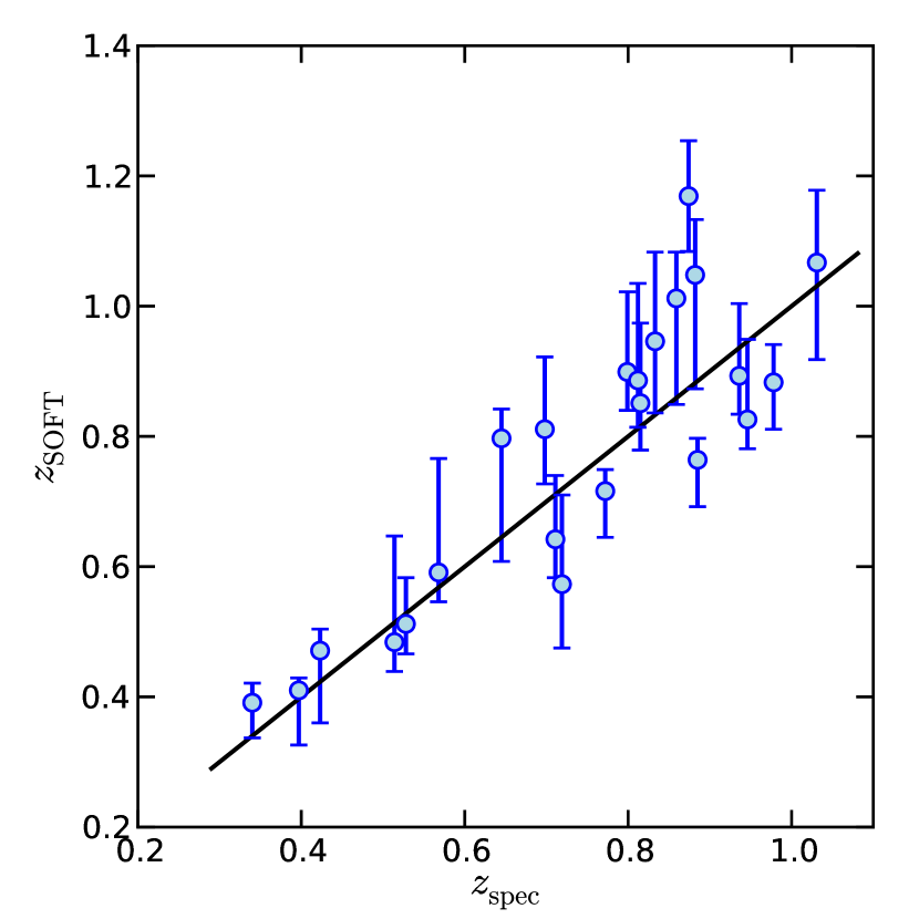
Figure 1: Comparison of the peak redshift estimates from SOFT against the spectroscopic redshift measurements for 23 TN SNe. The straight line shows perfect parity (z_SOFT=z_spec). The rms scatter about the line is 0.10, and the reduced $\chi^{2}$ statistic is 0.85.

The SOFT classification grades and redshift estimates for all 131 TN SN candidates are summarized in Table 2. For each SN in this table we have used the best available redshift measurement to inform the prior. The 23 spectroscopically confirmed SNe from Table 1 appear again in Table 2, now with updated classification grades and improved parameter estimates due to the addition of spectroscopic information. Also included are redshift priors derived from 14 likely SN host galaxies and photometric redshift estimates for a further 22 possible hosts (see the final two columns of Table 2). To account for possibile host galaxy mismatches, the floor of the Gaussian redshift prior has been raised to 10% of the peak value, spread across the width of the redshift parameter space.

Table 1: Redshift Validation Subset : 23 Spectroscopically Observed TN SNe

Name	RA(J2000)	DEC(J2000)	$\gamma_{\rm TN}$	$z_{\rm spec}$	$z_{\rm SOFT}$
SN2001fo	04:37:41.45	-01:29:33.1	1.000	0.772	0.716 ${}^{+0.033}_{-0.071}$
SN2001fs	04:39:30.68	-01:28:21.9	0.928	0.874	1.169 ${}^{+0.085}_{-0.085}$
SN2001hs	04:39:22.39	-01:32:51.4	0.998	0.833	0.946 ${}^{+0.137}_{-0.110}$
SN2001hu	07:50:35.90	+09:58:14.2	0.991	0.882	1.048 ${}^{+0.085}_{-0.175}$
SN2001hx	08:49:24.61	+44:02:22.4	0.999	0.799	0.899 ${}^{+0.123}_{-0.059}$
SN2001hy	08:49:45.85	+44:15:31.8	0.998	0.812	0.886 ${}^{+0.149}_{-0.072}$
SN2001iv	07:50:13.53	+10:17:10.4	1.000	0.397	0.410 ${}^{+0.019}_{-0.084}$
SN2001iw	07:50:39.32	+10:20:19.1	1.000	0.340	0.391 ${}^{+0.030}_{-0.054}$
SN2001ix	10:52:18.92	+57:07:29.6	0.921	0.711	0.642 ${}^{+0.098}_{-0.059}$
SN2001iy	10:52:24.28	+57:16:36.1	1.000	0.568	0.591 ${}^{+0.175}_{-0.045}$
SN2001jb	02:26:33.31	+00:25:35.0	0.936	0.698	0.811 ${}^{+0.111}_{-0.084}$
SN2001jf	02:28:07.13	+00:26:45.1	0.881	0.815	0.851 ${}^{+0.123}_{-0.072}$
SN2001jh	02:29:00.29	+00:20:44.2	1.000	0.885	0.764 ${}^{+0.033}_{-0.072}$
SN2001jm	04:39:13.82	-01:23:18.2	0.999	0.978	0.883 ${}^{+0.058}_{-0.072}$
SN2001jn	04:40:12.00	-01:17:45.9	0.897	0.645	0.797 ${}^{+0.045}_{-0.189}$
SN2001jp	08:46:31.40	+44:03:56.6	0.640	0.528	0.512 ${}^{+0.071}_{-0.046}$
SN2001kd	07:50:31.24	+10:21:07.3	0.934	0.936	0.893 ${}^{+0.111}_{-0.059}$
SN2002P	02:29:05.71	+00:47:20.1	0.772	0.719	0.573 ${}^{+0.137}_{-0.098}$
SN2002W	08:47:54.42	+44:13:42.9	0.822	1.031	1.067 ${}^{+0.111}_{-0.149}$
SN2002X	08:48:30.54	+44:15:35.3	0.939	0.859	1.012 ${}^{+0.071}_{-0.163}$
SN2002aa	07:48:45.28	+10:18:00.8	0.926	0.946	0.826 ${}^{+0.123}_{-0.045}$
SN2002ab	07:48:55.70	+10:06:06.3	0.993	0.423	0.471 ${}^{+0.033}_{-0.111}$
SN2002ad	10:50:12.19	+57:31:11.6	0.996	0.514	0.484 ${}^{+0.163}_{-0.045}$

Table 2: SOFT results for 131 TN SN Candidates

Name	RA(J2000)	DEC(J2000)	$\gamma_{\rm TN}$	$z_{\rm SOFT}$	$z_{\rm prior}$	$z_{\rm prior}$ Source
SN2001fi	02:26:38.87	+00:26:15.1	1.00	0.33 ${}^{+0.01}_{-0.01}$	0.320 $\pm$ 0.001	IAUC 7745
SN2001fk	02:28:04.70	+00:46:17.7	1.00	0.81 ${}^{+0.01}_{-0.01}$	0.804 $\pm$ 0.001	DEEP2
SN2001fn	02:29:00.49	+00:42:21.6	0.69	0.76 ${}^{+0.02}_{-0.04}$	0.186 $\pm 0.01$	IAUC 7745
SN2001fo	04:37:41.45	-01:29:33.1	1.00	0.77 ${}^{+0.01}_{-0.01}$	0.772 $\pm$ 0.001	B04
SN2001fq	04:38:04.51	-01:23:49.0	1.00	0.94 ${}^{+0.18}_{-0.06}$	0.01$\pm 0.01$	IAUC 7745
f0230a	02:26:09.11	+00:34:56.9	1.00	0.77 ${}^{+0.01}_{-0.01}$	0.771 $\pm$ 0.001	DEEP2
f0230b	02:27:26.13	+00:48:27.7	0.53	0.24 ${}^{+0.00}_{-0.02}$	$\cdots$
f0230c	02:27:54.90	+00:31:48.4	1.00	1.00 ${}^{+0.06}_{-0.10}$	$\cdots$
f0230e	02:28:21.92	+00:24:26.8	0.60	1.02 ${}^{+0.01}_{-0.01}$	1.014 $\pm$ 0.001	DEEP2
f0230f	02:29:35.86	+00:38:45.2	0.05	0.86 ${}^{+0.08}_{-0.06}$	$\cdots$

The majority of these 131 candidates are classified by SOFT as TN SNe: 90 objects have a TN SN classification grade above 50%, with 63 of those above 90%. This is, however, somewhat lower than the 98 objects identified as TN SNe in the BT06 analysis. As will be explained below, we include all 131 objects in our analysis, using the classification grades to account for uncertainty in sample selection. The mean redshift uncertainty determined by SOFT for the complete set is 0.055, broadly consistent with the scatter observed in Figure 1 and seen in the SOFT validation tests using SNe from the Sloan Digital Sky Survey (SDSS) and the Supernova Legacy Survey (SNLS) (Rodney & Tonry, 2010).

A handful of SN candidates in Table 2 show discrepancies between the redshift prior and the redshift estimate determined by SOFT. Three objects (f0848d, f0848f, f0848h) have marginally significant ($<2\sigma$) differences between the assumed host galaxy redshift and the SOFT redshift. These host galaxy redshift priors are taken from the SDSS photometric redshift catalog (Oyaizu et al., 2008) and have very large uncertainties ($\sigma_{z}\geq 0.1$), so we accept the SOFT distribution as a reasonable estimate. Two other objects (SN2001ft, f0848b) have SOFT redshifts that are significantly lower than the input redshift priors. Both of these objects have a classification grade of $\gamma_{\rm TN}$=0, indicating that SOFT strongly classifies them as CC SNe. In such cases the SOFT redshift estimation is very poor, because CC SNe are an inhomogeneous population that is only sparsely sampled by the SOFT template library. Our $\gamma_{\rm TN}$-weighted counting procedure (described in Section 4.1) ensures that these objects provide only a negligible contribution to the count of detected TN SNe. Three other objects (f0749t, f0848r, SN2001fn) have SOFT redshift estimates that are significantly higher than their priors. The priors for the first two are again from SDSS galaxies, and in this case both galaxies have $>5\arcsec$ separation from the position of the SN. We assume that these are foreground galaxies, and the actual hosts have a low surface brightness and are undetected by SDSS. The final object, SN2001fn, is well aligned with a galaxy in the SDSS that has a photometric redshift of 0.7$\pm$0.3, although the reported spectroscopic redshift of the host galaxy is 0.186. Even with a strong spectroscopic prior at z=0.186, SOFT finds a good classification for this object as a TN SN at a redshift of 0.76${}^{+0.02}_{-0.04}$ – in good agreement with the SDSS photo-z. Without conclusive evidence in either direction, we adopt the SOFT redshift estimate, noting that a change in the redshift of this single object does not significantly affect our final rate measurements.

4 The Revised IfA Deep TN SN Rate

The fundamental measurement needed to compute the TN SN rate as a function of redshift is simply a count of the number of detected SNe as a function of redshift: $N_{\rm det}(z)$. This count is computed in Section 4.1 for 9 redshift intervals reaching out to z=1.1. To convert this to a volumetric rate, the detection count at each redshift is divided by the control count, $N_{\rm ctrl}(z)={\rm SNuVol}\times V(z)\times t_{\rm ctrl}(z)$. Here $V(z)$ is the volume of the survey in the redshift range from $z$ to $z+dz$ and $t_{\rm ctrl}(z)$ is the effective survey period or control time: the total time span in which a TN SN exploding at redshift $z$ would be detectable by this survey. Thus, the control count gives the number of SN detections that would be expected from this survey if the SN rate per unit volume were constant at all redshifts, fixed at 1 SNuVol=10^-4 SNIa Mpc^-3 yr^-1 $h_{70}^{3}$. Simulations to compute $N_{\rm ctrl}(z)$ are described in Section 4.2.

4.1 The Detected Count

In the absence of a strong spectroscopic redshift prior, the redshift distributions produced by SOFT are typically broad and asymmetric, sometimes with multiple peaks - making it impossible to pin them down into any single redshift bin for counting. To incorporate these complex uncertainties into our TN SN detection counts, a Markov Chain Monte Carlo (MCMC) sampling test was executed for each SN, as illustrated in Figure 2. The MCMC provides 1000 redshift realizations for each SN, distributed so as to reconstruct the measured SOFT redshift distribution.

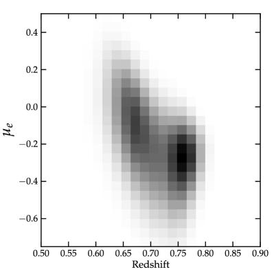
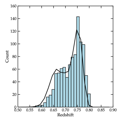
Figure 2: To tally the contribution from each individual SN candidate over a series of redshift bins, we utilize a Markov Chain Monte Carlo series, drawing 1000 random redshifts that reproduce the redshift distribution measured by SOFT. (a) The composite fuzzy membership function (equivalent of a posterior probability distribution) for SN f0230a in the (z,$\mu_{e}$) plane. (b) After marginalizing over $\mu_{e}$, the distribution in redshift (solid line) is used as the target distribution for our MCMC series. The blue histogram shows the results of 1000 MCMC draws, effectively reproducing the highly irregular probability distribution.

After repeating this for all candidates, we have 1000 sets of 131 redshift assignments, with each set representing a possible redshift distribution for the entire IFA Deep SN sample. To count the number of detected SNe, each set of 131 redshifts is binned into intervals of width $\Delta z$=0.1 from 0.0 to 1.4. To incorporate the uncertainty of classification into our counts, we allow each SN to contribute a fractional count to the redshift bin that it falls in for a given simulation. This fractional count is drawn from a Gaussian distribution centered on the composite TN SN classification grade, $\gamma_{\rm TN}$, with a width of $\sigma=0.05$. This 5% scatter reflects the uncertainty of the classification grades deduced from testing SOFT against validation data in Rodney & Tonry (2009). With each SN contributing a count of less than unity, the average of the total count across all redshifts is $\sum\gamma_{\rm TN}=84.5$, rather than 131.

After binning up all 1000 Monte Carlo realizations, we have 1000 measurements for the count in each bin. Taking the mean of this 1000-element vector gives us our central count estimate for that redshift interval, and the standard deviation provides an estimate of the statistical uncertainty that accounts for error in both the classification and the redshift estimation. The counts of detected SNe in each redshift bin are given in Table 3a, along with the statistical and systematic uncertainties (described in Section 5).

Table 3: New Determination of IfA Deep TN SN Rates

$z$	Detected Count				Control Count		SN Rate
	$N_{\rm det}$	$\delta N_{z}$	$\delta N_{\rm Poiss}$	$(\delta N_{\rm syst})$	$N_{\rm ctrl}$	$(\delta N_{\rm syst})$	SNR	$\delta$SNRstat	($\delta$SNRsyst)
0.15	1.95	$\pm$0.12	$\pm$1.40	$\left({}^{+0.04}_{-0.32}\right)$	6.1	$\left({}^{+0.6}_{-1.3}\right)$	0.32	$\pm$0.23	$\left({}^{+0.07}_{-0.06}\right)$
0.35	4.01	$\pm$0.91	$\pm$2.00	$\left({}^{+0.29}_{-0.00}\right)$	11.7	$\left({}^{+1.2}_{-2.2}\right)$	0.34	$\pm$0.19	$\left({}^{+0.07}_{-0.03}\right)$
0.45	5.11	$\pm$1.14	$\pm$2.26	$\left({}^{+1.74}_{-0.16}\right)$	16.6	$\left({}^{+2.2}_{-3.0}\right)$	0.31	$\pm$0.15	$\left({}^{+0.12}_{-0.04}\right)$
0.55	6.49	$\pm$1.42	$\pm$2.55	$\left({}^{+0.17}_{-1.30}\right)$	20.4	$\left({}^{+2.3}_{-4.3}\right)$	0.32	$\pm$0.14	$\left({}^{+0.07}_{-0.07}\right)$
0.65	10.09	$\pm$1.75	$\pm$3.18	$\left({}^{+0.95}_{-1.09}\right)$	20.8	$\left({}^{+2.5}_{-5.5}\right)$	0.49	$\pm$0.17	$\left({}^{+0.14}_{-0.08}\right)$
0.75	14.29	$\pm$2.19	$\pm$3.78	$\left({}^{+0.60}_{-2.03}\right)$	20.9	$\left({}^{+3.0}_{-7.0}\right)$	0.68	$\pm$0.21	$\left({}^{+0.23}_{-0.14}\right)$
0.85	15.43	$\pm$2.09	$\pm$3.93	$\left({}^{+1.78}_{-0.00}\right)$	19.9	$\left({}^{+4.1}_{-7.7}\right)$	0.78	$\pm$0.22	$\left({}^{+0.31}_{-0.16}\right)$
0.95	13.21	$\pm$2.31	$\pm$3.63	$\left({}^{+0.32}_{-1.43}\right)$	17.3	$\left({}^{+5.7}_{-7.1}\right)$	0.76	$\pm$0.25	$\left({}^{+0.32}_{-0.26}\right)$
1.05	11.01	$\pm$2.08	$\pm$3.32	$\left({}^{+1.28}_{-1.83}\right)$	13.9	$\left({}^{+6.8}_{-6.1}\right)$	0.79	$\pm$0.28	$\left({}^{+0.36}_{-0.41}\right)$

4.2 The Control Count

The second component of the TN SN rate calculation, $N_{\rm ctrl}$, is derived from a Monte Carlo simulation of $\sim$5000 SNe that replicates the IfA Deep survey observations. The simulation is defined over a grid of redshift values from $z=0.01$ to 1.6 in steps of $\delta z=0.02$. At each point on the grid we compute $N_{\rm exp}(z)$, the total number of SNe that explode each year within the IfA Deep survey area in a shell of thickness $\delta z$. This number is calculated as $N_{\rm exp}(z)=1~{}{\rm SNuVol}\times V(z)\times 1~{}{\rm yr}$. Here $V(z)$ is the volume of a shell at redshift $z$, using a total survey area of 2.29 square degrees and assuming a $\Lambda{\rm CDM}$ cosmology.

Having computed the total number of explosions for each point on the redshift grid, we now want to simulate how these SNe would be distributed in magnitude space. We assume a luminosity function for the TN SN population composed of three Gaussian distributions representing the overluminous objects (Ia$+$ or SN 1991T-like), which make up 20% of the population, normal Ia’s at 64%, and underluminous TN SNe (Ia$-$ or SN 1991bg-like) comprising 16% (Li et al., 2001). The Gaussians have $\sigma=$0.45, 0.30, and 0.50 magnitudes for the Ia$+$, Ia, and Ia$-$ components, respectively. The same luminosity function is used for all redshift bins.

Each of the $\sim$5000 simulated SNe now has an assumed redshift $z$ and a peak magnitude $m_{\rm pk}$ drawn from the luminosity functions. These parameters are then applied to construct a model light curve using the apparatus of the SOFT template library (Rodney & Tonry, 2009). The simulated light curve includes cosmological dimming appropriate for the redshift by assuming a $\Lambda{\rm CDM}$ cosmology, as well as extinction due to host galaxy dust that is drawn from a “galactic line of sight” distribution (Hatano et al., 1998) as implemented in Tonry et al. (2003) and Wood-Vasey et al. (2007). Briefly, we draw a host extinction value for each simulated SN from a probability distribution constructed by assuming that 25% of hosts are bulge systems and 75% are disk systems. The extinction distribution curves of Hatano et al. (1998) are approximated by $f(A_{B})\propto 0.02\delta(A_{B})+10^{-1.25-A_{B}}$ for bulge systems and $f(A_{B})\propto 0.02\delta(A_{B})+e^{-3.77-A_{B}^{2}}$ for disk systems.

The control time $t_{ctrl}(z,m_{\rm pk})$ for this model light curve is calculated by counting the days on which this SN could explode and subsequently be detected by the IfA Deep survey. To determine if a model SN would be detected, we count up the number of IfA Deep observation epochs for which the synthetic light curve is brighter than the detection threshold. If the tally of detection epochs is $\geq 5$ then we consider this SN to be detected.

Multiplying together the number of SN explosions $N_{exp}(z,m_{pk})$ per year and the control time $t_{ctrl}(z,m_{pk})$ gives us a final estimate for the control count of SN detections $N_{ctrl}(z,m_{pk})$. Integrating over all possible peak magnitudes gives us the final control count of TN SN detections in each redshift bin, presented in Table 3b. The systematic uncertainty estimates included in Table 3 are derived in the following section.

5 Systematic Uncertainty Estimates

Both of the principle components of our rate calculation – the detection count and the control count – can potentially introduce systematic errors into the SN rate values. A suite of systematic uncertainty tests were performed in which a parameter of interest was adjusted, the classification and redshift estimation were repeated for all candidates, and new rate estimates were measured. The difference between the revised rate and our baseline rate measurement was taken as the systematic error estimate, separately for each redshift bin. All tests are described below, and the resulting uncertainty estimates are reported in Table 4.

5.1 Systematic Errors in $N_{det}$

Peculiar SNe: If a normal TN SN gets matched by a highly peculiar SN template we could derive an erroneous redshift. We don’t expect a significant number of peculiar Ia’s in a survey of this size. This systematic test removes the very unusual SN 2000cx and SN2002cx from the SOFT template library.

Host Galaxy Dust: First, we change the ratio of total to selective extinction to R_V=2.1, accommodating the possibility that dust around extragalactic SNe is very different from the Milky Way extinction law of R_V=3.1 (Astier et al., 2006; Kowalski et al., 2008; Kessler et al., 2009; Poznanski et al., 2009). Next, we change the prior on the extinction parameter A_V from the “Galactic Line of Sight” prior to an exponential distribution $p({\mbox{A${}_{V}$}})\propto\exp(-{\mbox{A${}_{V}$}}/5)$ that approximates the extreme inclination models of Riello & Patat (2005), following Neill et al. (2006).

Redshift Prior: For objects without a spectroscopic redshift measurement or a host galaxy photo-$z$, we have relied on a redshift prior that scales with the cosmological volume element, going as $z^{2}$. This can introduce a systematic bias towards higher $z$ estimates. An alternative and differently biased redshift prior can be derived from the control count, as given in Table 3. The control count vs. z for this survey is well approximated by a Gaussian with $\mu=0.7$ and $\sigma=0.38$, so we estimate the systematic uncertainty by using this function for the redshift prior.

“Fuzzy AND” Rejection Threshold As detailed in Rodney & Tonry (2010), the SOFT redshift estimate for any candidate SN is derived by combining the fuzzy membership functions from multiple templates using the Fuzzy AND operation. To prevent the combination from being dominated by extreme outliers, we have used a rejection threshold of 5% on the integrated membership grade $\gamma_{TN}$. To test whether this value is introducing systematic effects, we reprocessed the SN light curves using threshold values of 3% and 10%.

Table 4: Systematic Uncertainty Estimates

	(a) Change in Detected Count
Redshift:	0.25	0.35	0.45	0.55	0.65	0.75	0.85	0.95	1.05
drop peculiar templates	$-0.00$	$+0.02$	$+0.72$	$+0.00$	$-0.69$	$+0.22$	$+0.06$	$-1.33$	$+0.93$
change $R_{V}$ by 1	$-0.32$	$+0.14$	$+1.42$	$+0.17$	$-0.72$	$-0.89$	$+0.08$	$-0.34$	$+0.20$
flat AV prior	$+0.04$	$+0.20$	$+0.71$	$-0.32$	$+0.00$	$-0.50$	$+0.71$	$-0.39$	$-0.77$
Gaussian $z$ prior	$+0.01$	$+0.10$	$-0.06$	$-0.08$	$+0.34$	$-0.52$	$+0.13$	$-0.02$	$-0.02$
modified fuzzy AND threshold	$+0.00$	$+0.11$	$-0.15$	$-1.26$	${}^{+0.89}_{-0.46}$	${}^{+0.56}_{-1.67}$	$+1.63$	${}^{+0.32}_{-0.04}$	${}^{+0.85}_{-1.66}$
TOTAL :	$+0.04$	$+0.29$	$+1.74$	$+0.17$	$+0.95$	$+0.60$	$+1.78$	$+0.32$	$+1.28$
	$-0.32$	$-0.00$	$-0.16$	$-1.30$	$-1.09$	$-2.03$	$-0.00$	$-1.43$	$-1.83$
	(b) Change in Control Count
Redshift:	0.25	0.35	0.45	0.55	0.65	0.75	0.85	0.95	1.05
Alternate SN luminosity function	$+0.2$	$+0.4$	$+1.0$	$+0.4$	$+0.5$	$+0.0$	$+0.0$	$+0.0$	$+0.3$
	$-0.3$	$-0.5$	$-0.5$	$-1.1$	$-0.8$	$-0.7$	$-1.2$	$-1.1$	$-1.5$
Minimum no. detections $\pm$ 1	$+0.55$	$+1.1$	$+1.95$	$+2.3$	$+2.45$	$+3.05$	$+4.1$	$+5.65$	$+6.8$
	$-1.05$	$-1.8$	$-2.25$	$-2.6$	$-3.15$	$-4.45$	$-5.6$	$-5.7$	$-5.15$
Filling factor $\pm$ 4%	$+0.00$	$+0.05$	$+0.15$	$+0.0$	$+0.0$	$+0.0$	$+0.0$	$+0.0$	$+0.0$
	$-0.35$	$-0.55$	$-0.75$	$-1.5$	$-1.45$	$-1.85$	$-2.05$	$-1.65$	$-1.35$
Exponential dust profile	$-0.65$	$-1.1$	$-1.7$	$-2.9$	$-4.2$	$-5.1$	$-4.8$	$-3.8$	$-2.5$
TOTAL :	$+0.59$	$+1.17$	$+2.20$	$+2.33$	$+2.50$	$+3.05$	$+4.10$	$+5.65$	$+6.81$
	$-1.32$	$-2.24$	$-2.96$	$-4.32$	$-5.47$	$-7.02$	$-7.75$	$-7.13$	$-6.07$

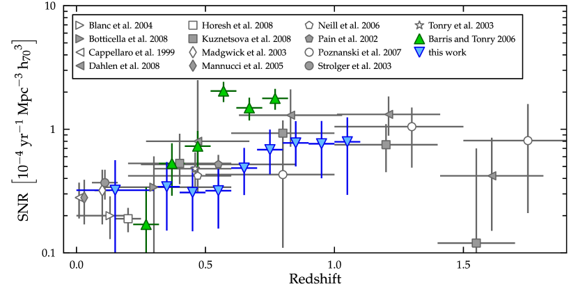
Figure 3: Results of the final TN SN rate calculation. The original IFA Deep rates (BT06) are shown as upward-pointing green triangles. The new rate measurements described here are plotted as downward-pointing blue triangles. Error bars on the new rate points include both statistical and systematic uncertainties. A compilation of rates from the literature are plotted as gray symbols, with references as given in the legend.

5.2 Systematic Errors in $N_{\rm ctrl}$

TN SN Luminosity Function: There is substantial uncertainty in the balance of the SN luminosity function between the overluminous Ia$+$, the normal Ia, and the underluminous Ia$-$ sub-classes, provided by Li et al. (2001). We first modify the baseline (20%, 64%, 16%) to (13%, 77%, 10%) and then to (27%, 51%, 22%).

Detection Thresholds: The actual process of extracting 131 likely TN SN candidates from among the many thousands of potential transient objects in the IfA Deep survey was quite complex (for details see Barris (2004)). Our proxy for the selection process used the simple requirement that a SN must be above the 5-$\sigma$ point source threshold in 5 epochs in order to be counted. Our systematic test modifies this to 4 and then 6 epochs. The reported systematic error estimate is half of the difference between the baseline and the modified control count.

Survey Area: The computation of the survey area was greatly simplified in our Monte Carlo procedure by assuming a 90% filling factor for volume calculations. We recomputed the control count using alternate filling factors of 86% and 94%.

Host Galaxy Dust: As in the detected count systematic uncertainty test above, we modify the host galaxy dust first to use $R_{V}=2.1$ and then to follow an exponential $A_{V}$ distribution.

6 Results

A summary of the principal components of the SN Rate calculation is given in Table 3. The final tally of the number of detected TN SNe is given in column 2, with statistical and systematic uncertainties in columns 3–5. The control count of TN SNe is given in column 6, followed by systematic uncertainty estimates. The resulting SN Rate numbers and associated uncertainties appear in the final three columns.

These revised rate estimates are significantly different from the numbers derived in BT06. These differences arise from improvements in both the measurement of $N_{det}$ and the calculation of $N_{ctrl}$. With an improved SN light curve analysis program in SOFT, we now have more robust photometric redshift estimates and classification grades for all 131 SNe. SOFT also has new access to more detailed prior information with the addition of 36 host galaxy redshift measurements from spectra and photo-z’s. These improvements have allowed us to reliably extend the rate estimate beyond the z=0.75 limit applied by BT06, reaching now out to a mean redshift of 1.05 in the final bin.

Using an updated Monte Carlo simulation, we have generated a revised control count for the number of SNe detectable by the IfA Deep survey as a function of redshift. Our simulations consistently disagree with BT06 in that we compute a larger control count in every one of the redshift bins. However, we have also performed a series of systematic uncertainty tests, and we find that when systematic errors are included, our control counts are consistent with those from BT06.

In Figure 3 we show the final rate measurements from the IfA Deep survey, compared to other rates from the literature. The original IfA Deep rates are shown in green, and the newly derived rates are plotted in blue. A compilation of rates from the literature is plotted in the background in gray. The new IfA rate measures are clearly in much better agreement with the consensus of literature rates than were the BT06 values. Our new IfA results indicate that the TN SN rate increases with redshift out to at least z=1.0, with no evidence of reaching a peak in the redshift range sampled.

References

- Astier et al. (2006) Astier, P., et al. 2006, A&A, 447, 31
- Barris (2004) Barris, B. J. 2004, PhD thesis, University of Hawai’i
- Barris & Tonry (2006) Barris, B. J., & Tonry, J. L. 2006, ApJ, 637, 427
- Barris et al. (2004) Barris, B. J., et al. 2004, ApJ, 602, 571
- Barris et al. (2005) Barris, B. J., Tonry, J. L., Novicki, M. C., & Wood-Vasey, W. M. 2005, AJ, 130, 2272
- Blanc et al. (2004) Blanc, G., et al. 2004, A&A, 423, 881
- Botticella et al. (2008) Botticella, M. T., et al. 2008, A&A, 479, 49
- Cappellaro et al. (1999) Cappellaro, E., Evans, R., & Turatto, M. 1999, A&A, 351, 459
- Dahlen et al. (2008) Dahlen, T., Strolger, L.-G., & Riess, A. G. 2008, ApJ, 681, 462
- Hatano et al. (1998) Hatano, K., Branch, D., & Deaton, J. 1998, ApJ, 502, 177
- Horesh et al. (2008) Horesh, A., Poznanski, D., Ofek, E. O., & Maoz, D. 2008, MNRAS, 389, 1871
- Kessler et al. (2009) Kessler, R., et al. 2009, ApJS, 185, 32
- Komatsu et al. (2010) Komatsu, E., et al. 2010, ArXiv e-prints
- Kowalski et al. (2008) Kowalski, M., et al. 2008, ApJ, 686, 749
- Kuznetsova et al. (2008) Kuznetsova, N., et al. 2008, ApJ, 673, 981
- Li et al. (2001) Li, W., Filippenko, A. V., Treffers, R. R., Riess, A. G., Hu, J., & Qiu, Y. 2001, ApJ, 546, 734
- Liu et al. (2002) Liu, M. C., Wainscoat, R., Martín, E. L., Barris, B., & Tonry, J. 2002, ApJ, 568, L107
- Madgwick et al. (2003) Madgwick, D. S., Hewett, P. C., Mortlock, D. J., & Wang, L. 2003, ApJ, 599, L33
- Mannucci et al. (2005) Mannucci, F., Della Valle, M., Panagia, N., Cappellaro, E., Cresci, G., Maiolino, R., Petrosian, A., & Turatto, M. 2005, A&A, 433, 807
- Neill et al. (2006) Neill, J. D., et al. 2006, AJ, 132, 1126
- Oyaizu et al. (2008) Oyaizu, H., Lima, M., Cunha, C. E., Lin, H., Frieman, J., & Sheldon, E. S. 2008, ApJ, 674, 768
- Pain et al. (2002) Pain, R., et al. 2002, ApJ, 577, 120
- Poznanski et al. (2009) Poznanski, D., et al. 2009, ApJ, 694, 1067
- Poznanski et al. (2007) —. 2007, MNRAS, 382, 1169
- Riello & Patat (2005) Riello, M., & Patat, F. 2005, MNRAS, 362, 671
- Rodney & Tonry (2009) Rodney, S. A., & Tonry, J. L. 2009, ApJ, 707, 1064
- Rodney & Tonry (2010) —. 2010, ApJ, 715, 323
- Strolger (2003) Strolger, L. 2003, PhD thesis, University of Michigan
- Tonry et al. (2003) Tonry, J. L., et al. 2003, ApJ, 594, 1
- Wood-Vasey et al. (2007) Wood-Vasey, W. M., et al. 2007, ApJ, 666, 694