Simulation of Edge Localised Modes using BOUT++

Abstract

The BOUT++ code is used to simulate ELMs in a shifted circle equilibrium. Reduced ideal MHD simulations are first benchmarked against the linear ideal MHD code ELITE, showing good agreement. Diamagnetic drift effects are included finding the expected suppression of high toroidal mode number modes. Nonlinear simulations are performed, making the assumption that the anomalous kinematic electron viscosity is comparable to the anomalous electron thermal diffusivity. This allows simulations with realistically high Lundquist numbers ($S=10^{8}$), finding ELM sizes of 5-10% of the pedestal stored thermal energy. Scans show a strong dependence of the ELM size resistivity at low Lundquist numbers, with higher resistivity leading to more violent eruptions. At high Lundquist numbers relevant to high-performance discharges, ELM size is independent of resistivity as hyper-resistivity becomes the dominant dissipative effect.

1 Introduction

Future tokamak devices such as ITER and DEMO require high performance plasma operation in order to demonstrate economical fusion performance. For this reason, discharges with a transport barrier close to the plasma edge (H-mode [1]) are the current baseline operating scenario for ITER [2]. Whilst transport barriers at the plasma edge result in improved performance, the steep pressure gradients and associated bootstrap current can destabilise peeling-ballooning modes [3]. These ideal MHD instabilities are thought to be responsible for triggering the observed eruptions of filamentary structures from the plasma edge known as Edge Localised Modes (ELMs). The particles and energy released during ELMs are deposited on material surfaces and are potentially damaging in future devices. There is therefore interest in understanding and controlling these events.

Understanding of the linear onset and structure of peeling-ballooning modes is now quite well developed, with codes such as ELITE [3, 4], GATO [5] and MISHKA [6, 7] able to predict experimental operating limits[3, 8, 9]. Study of the nonlinear evolution of these instabilities is more challenging, and although there are analytic theories [10] and semi-analytic models [11, 12] for the early non-linear evolution, it is not yet fully understood how this develops into the filamentary structures observed, and ultimately how particles and energy are lost.

Several 3D non-linear codes have been used to simulate ELMs, including NIMROD [13, 14, 15, 16], BOUT [17, 18], JOREK [19, 20, 21], GEM [22, 23], M3D [24, 25, 26] and M3D-C1 [27]. These codes incorporate a wide range of physics including (in the case of BOUT and some NIMROD simulations) 2-fluid effects. In this paper, simulations of ELMs using the the BOUT++ code [28] based on modified reduced MHD in a shifted circle equilibrium are presented, expanding on and extending results presented in [29]. By introducing a hyper-resistive term into Ohm’s law, realistic resistivities have been simulated, and the effect of varying resistivity on ELM sizes has been investigated.

Section 2 describes the starting set of equations used for comparison with linear ideal MHD, and the equilibrium simulated is described in section 3. A novel means to handle the vacuum region which has been found to work well in ideal or resistive MHD simulations is described in section 2.1. Linear simulations are benchmarked against linear ideal MHD codes in section 4, and nonlinear simulations of ideal reduced MHD and the issues encountered are discussed in section 5. By incorporating diamagnetic drift and either high resistivity or a hyper-resistivity, simulations of nonlinear eruptions are performed and discussed in sections 6 and 7 respectively. The effect of varying resistivity on ELM crash size is then discussed in more detail in section 8. Details of the magnetic field structure are presented in section 9, indicating a reconnection of flux-surfaces at the leading edges of the erupting filaments.

2 Model equations

In this paper, the starting equations are those of high-$\beta$ reduced MHD [30], evolving pressure $P$, vorticity $U$ and magnetic potential $\psi=A_{||}/B_{0}$:

$$\rho\frac{dU}{dt} = B^{2}\mathbf{b}\cdot\nabla\left(\frac{J_{||}}{B}\right)+2\mathbf{b}_{0}\times\mathbf{\kappa}_{0}\cdot\nabla P$$ (1)

$$\frac{\partial\psi}{\partial t} = -\frac{1}{B_{0}}\nabla_{||}\phi$$ (2)

$$\frac{\partial P}{\partial t} = -\frac{1}{B_{0}}\mathbf{b}_{0}\times\nabla\phi\cdot\nabla P$$ (3)

$$U = \frac{1}{B_{0}}\nabla_{\perp}^{2}\phi$$ (4)

$$J_{||} = J_{||0}-\frac{1}{\mu_{0}}B_{0}\nabla_{\perp}^{2}\psi$$ (5)

where $\nabla_{||}F=B\partial_{||}\left(F/B\right)$ for any $F$, $\partial_{||}=\left(\mathbf{b}_{0}+\mathbf{b}_{1}\right)\cdot\nabla$, $\mathbf{b}=\mathbf{B}/B$. The plasma density is constant in space and time, fixed at $10^{19}$m^-3. The perturbed magnetic field is given by $\mathbf{B}_{1}=\nabla\psi\times\mathbf{B}_{0}$ where $\mathbf{B}_{0}$ is the unperturbed field. $\kappa_{0}=\mathbf{b}_{0}\cdot\nabla\mathbf{b}_{0}$ is the field curvature and all quantities are in SI units. The vorticity equation 1 includes the kink/peeling term through the perturbed magnetic field:

$$\mathbf{b}\cdot\nabla\left(\frac{J_{||}}{B_{0}}\right)=\left(\mathbf{b}_{0}\cdot\nabla-\mathbf{b}_{0}\cdot\nabla\psi\times\nabla\right)\left(\frac{J_{||}}{B_{0}}\right)$$

This minimal set of equations contains the basic physics needed to describe peeling-ballooning modes, including pressure/curvature and parallel current (kink/peeling) instability drives, and field-line bending stabilisation. The model is a useful starting point because it allows benchmarking against linear ideal MHD codes such as ELITE, providing a valuable means of checking the results of these simulations.

In the pedestal with steep pressure gradients diamagnetic effects are expected to be significant, and damp high toroidal mode-number,$n$, instabilities which can lead to problems in ideal MHD simulations (see section 5). Therefore, the set of equations (1-5) is modified in section 6 to include the diamagnetic drift.

Dirichlet (zero value) boundary conditions are used for the perturbed pressure, vorticity and parallel current. To be consistent, the boundary conditions for $\psi$ and $\phi$ must satisfy $\nabla_{\perp}^{2}\psi=0$ and $\nabla_{\perp}^{2}\phi=0$. This is done by solving for each toroidal mode-number which have solutions $\hat{\phi}_{n}\simeq C_{+}\exp\left(\sqrt{g^{\zeta\zeta}/g^{\psi\psi}}k_{\zeta}x\right)+C_{-}\exp\left(-\sqrt{g^{\zeta\zeta}/g^{\psi\psi}}k_{\zeta}x\right)$ where $\zeta$ is the toroidal angle, $k_{\zeta}=n/R$ and $x$ is the radial ($\psi$) coordinate. Only solutions which decay going out of the domain are allowed, so $C_{+}=0$ on the outer boundary, and $C_{-}=0$ on the inner boundary.

2.1 Vacuum region

A complication of simulating the plasma edge region is the handling of the vacuum region, and the plasma-vacuum interface. In linear codes such as ELITE an analytical approach can be used; non-linear codes must also handle motion of the vacuum interface. The usual approach has been to treat the vacuum as a resistive plasma, with a jump in resistivity between plasma and vacuum [16]. Here a different approach is used: in the vacuum we evolve $\psi$ towards a self-consistent solution determined by currents in the core only. The procedure is as follows.

First define a smoothed step function $\Theta$, which switches between $0$ in the core to $1$ in the vacuum:

$$\Theta=\frac{1}{2}\left[1-\tanh\left(\frac{P-P_{vac}}{\Delta P_{vac}}\right)\right]$$ (6)

where $P_{vac}$ is the pressure at the plasma-vacuum interface, and $\Delta P_{vac}<P_{vac}$ is the transition width. At any given time, the solution $\psi\left(\mathbf{x},t\right)$ gives a current $J_{||}^{sol}$

$$J_{||}^{sol}=-\frac{1}{\mu_{0}}B_{0}\nabla_{\perp}^{2}\psi$$

which may or may not include currents in the vacuum region. From this, a “target” current $J_{||}^{target}$ is calculated by setting all vacuum currents to zero

$$J_{||}^{target}=J_{||}^{sol}\left(1-\Theta\right)$$

This is the closest physically acceptable solution to the current result. From this, a target $\psi$ can be calculated

$$\psi^{target}=\nabla_{\perp}^{-2}\left(\mu_{0}J_{||}^{target}/B_{0}\right)$$

In the vacuum region, this is the solution which would give zero current, but simply setting $\psi$ to this value in the vacuum would result in an inconsistency because $\psi$ in the core is affected by currents in the vacuum. Instead, equation 2 is modified to

$$\frac{\partial\psi}{\partial t}=-\left(1-\Theta\right)\frac{1}{B_{0}}\nabla_{||}\phi+\Theta\left(\psi^{target}-\psi\right)/\tau_{jvac}$$

and so $\psi$ converges on the target value with a small time-constant $\tau_{jvac}$. $\psi$ therefore evolves to a self-consistent state with zero current in the vacuum region.

This method has been found to work well for ideal and resistive simulations, even in the nonlinear regime. It is useful because this method uses the same code already used for solving the reduced MHD model with minimal modifications. At this point this method does not work once diamagnetic effects are included and so is not used in the nonlinear results presented in sections 6 and 7.

3 Equilibrium

Simulation of ELMs in full x-point geometry is necessary in order to predict the behaviour of ELMs in future devices. As a starting point however, it is useful to use equilibria which remove many of the complications of real magnetic geometry: This simplifies study of the basic physics of ELMs, but more importantly enables accurate benchmarking of the results against linear theory and other codes.

A test case which is becoming standard in this field is the cbm18 series, created by P.Snyder using the TOQ equilibrium code. The case used here cbm18_dens8 has now been used by NIMROD [16] and M3D-c1 [27] to benchmark linear growth-rates against the ELITE [3, 4] and GATO [5] linear MHD stability codes. The pressure and current profiles are shown in figure 1(a) over the range of normalised $\psi$ simulated using BOUT++ ($0.4<\psi_{n}<1.2$).

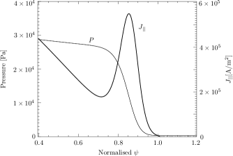
(a) Pressure and $J_{||}$ profiles

(b) Poloidal cross-section. Radial mesh coarsened for clarity

Figure 1: Equilibrium (cbm18_dens8) profiles and mesh

The definition of the plasma edge is somewhat arbitrary since here there are no separatrices, and so $\psi_{n}=1$ is defined as the point where the equilibrium plasma pressure gradient falls to zero. For this equilibrium, the normalised beta is $\beta_{N}=1.51$, edge $q_{a}=3.03$, pedestal toroidal pressure $\beta_{t0}=1.9\times 10^{-2}$ and normalised pedestal width is $L_{ped}/a=0.049$.

The mesh used for the simulations in this paper is shown in figure 1(b). This has a resolution of 512 points in radial coordinate $\psi$ and 64 in poloidal coordinate $\theta$. In the toroidal direction 64 points are usually used, with the results checked by doubling this to 128. Note that despite this relatively low resolution in $\theta$, high $m$ numbers can be simulated. This is because the field-aligned coordinate system

$$x=\psi-\psi_{0}\qquad y=\theta\qquad z=\phi-\int_{\theta_{0}}^{\theta}\nu\left(\psi,\theta\right)d\theta$$

(where $\nu\left(\psi,\theta\right)$ is the field-line pitch) means that the $\theta$ direction is aligned with the magnetic field and so $n_{\theta}=64$ is therefore the number of points along a field-line per poloidal turn. The effective poloidal resolution depends on the toroidal resolution (number of field-lines simulated $\times$ number of repetitions in a full torus) and the local safety factor $q\sim q_{a}=3.03$, and so is $\simeq 3\times 64\times 5=960$ for the simulations shown here.

In order to avoid problems associated with magnetic shear and deformation of grid cells associated with field-aligned coordinate systems, shifted local coordinate systems [31, 32] are used so that the radial derivative is always taken in $\psi$. Further details of this coordinate system and its implementation in BOUT++ can be found in [28].

4 Linear benchmarking

In order to benchmark BOUT++, linear simulations have been performed and comparison made to the ELITE [3, 4] and GATO [5] linear ideal MHD codes. Figure 2 shows the linear growth-rate from BOUT++ for this equilibrium (star symbols), along with the results from ELITE (open circles) and GATO (filled squares).

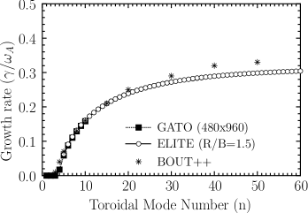
Figure 2: Linear growth rate of a strongly ballooning test case, as calculated by BOUT++ and the linear ideal MHD codes ELITE and GATO

All growth-rates are normalised to an Alfvén frequency $\omega_{A}=V_{A}/R$ , with $V_{A}$ the Alfvén velocity, and $R$ the major radius. For all the simulations presented in this paper, a reference density of $10^{19}$m^-3 was used, so that time is normalised to $\tau_{A}=0.37\mu$s.

At high-$n$, the BOUT++ result begins to deviate from the ELITE result, whereas it might be expected that finite-$n$ corrections would lead to the greatest differences being at low $n$. The reason for this is that as the mode number $n$ is increased the radial width of the mode becomes narrower: Since these simulations all used the same radial resolution, at high $n$ small-scale structures can no longer be resolved properly. The mode structure of the radial displacement $\xi_{\psi}$ from ELITE and BOUT++ have also been compared [28], finding good agreement. Individual $\left(m,n\right)$ modes are found to peak close to their resonant magnetic surfaces, as is expected from analytic theory. This test is a proof-of-principle which demonstrates that BOUT++ is capable of simulating the ideal ballooning mode correctly using ideal reduced MHD. Linear benchmarks are a necessary but not sufficient condition for non-linear results: comparisons against other nonlinear codes and ultimately experimental results are needed to verify the fidelity of nonlinear results.

5 Non-linear ideal MHD

In ideal MHD linear simulations, peaks in the parallel current form at rational $q$ surfaces. The width of these current sheets is of the order of the distance between rational surfaces $\Delta_{q}\sim r/nqs\simeq 6$mm, which can be resolved in the linear regime since when using 512 radial points across the pedestal the grid spacing is $\sim 1.1$mm. Linear codes such as ELITE and MARS [33] typically pack mesh-points around rational surfaces to handle these features, but this becomes much more challenging in the nonlinear regime: flux-surfaces move over time, current sheets can be compressed so reducing scale lengths, and any adaptive scheme will struggle to handle highly nonlinear regimes where flux surfaces may be destroyed.

Nonlinear simulations of ideal MHD have been attempted using BOUT++, but as yet without success: As flux-surfaces are distorted, small-scale structures are generated in the binormal direction which corresponds to the generation of high toroidal mode-numbers. The size of the structures formed in the toroidal direction is approximately given by rotating the radial scales in the perpendicular plane, and projecting in the toroidal direction which gives $L_{\zeta}\simeq\Delta B_{\zeta}/B_{\theta}\sim 5$cm and so a maximum toroidal mode-number of $n_{max}\sim 600$.

A second source of high-$k$ structures and hence numerical problems is that the modes with the highest growth-rate are those with the highest $n$ (i.e. those at the grid scale). Any perturbation at high $n$ will therefore rapidly grow and eventually dominate the solution.

Handling small-scale structures is a problem in many nonlinear simulations, and if possible then these should be resolved. In practice however, it is often necessary to add some sort of numerical dissipation to remove structures at the grid scales. Several approaches are commonly used to achieve this. For example the solution can be filtered in Fourier space (so only the low-$n$ modes are simulated) or a hyper-diffusion like term can be added. Whichever method is used, it should be chosen to minimise the impact on the large-scale structures of interest.

Tokamak simulations have the advantage that Larmor radius effects should naturally damp high-$k$ structures. Adding $\rho_{i}$ effects such as diamagnetic drifts both make the simulation more realistic and also aid numerical stability by damping high-$k$ structures. In this paper, nonlinear simulations are performed by first adding diamagnetic drift and following the common practice of incorporating a high resistivity in section 6, before introducing a hyper-resistive term in section 7.

6 Diamagnetic and resistive simulations

For these initial nonlinear simulations, the basic effects of diamagnetic stabilisation are incorporated into the model by modifying the vorticity (4) so that the total plasma velocity is now given by the sum of $E\times B$ and diamagnetic drifts.

$$\mathbf{V}\simeq\mathbf{V}_{E}+\mathbf{V}_{D}=\frac{1}{B^{2}}\mathbf{B}\times\nabla\phi+\frac{1}{enB^{2}}\mathbf{B}\times\nabla P$$

Hence assuming constant mass density $n$, this gives

$$U=\frac{1}{B}\nabla_{\perp}^{2}\left(\phi+\frac{P}{en}\right)$$ (7)

In this simplified model, both equilibrium and turbulent zonal ($m=n=0$) flows have been set to zero: $\mathbf{V}_{E0}+\mathbf{V}_{D0}=0$ and toroidally-averaged $\left<\delta\mathbf{v}_{E}+\delta\mathbf{v}_{D}\right>=0$. The equilibrium radial electric field is therefore given by $E_{r0}=\left(1/n_{0}Z_{i}e\right)\nabla_{r}P_{i0}$ (with $P_{i0}=P_{0}/2$) and perturbed radial electric field $\left<E_{r}\right>=\left(1/n_{0}Z_{i}e\right)\nabla_{r}\left<P_{i}\right>$. Recent work [20, 21, 34] indicates that the nonlinear formation of zonal flows results in multiple filaments breaking off from the plasma, but investigation of this effect is beyond the scope of this paper and the subject of future work.

At realistic resistivities of $S\sim 10^{8}$, the scale of the current sheets is limited by resistivity to approximately $\Delta_{R}\simeq R\sqrt{\left(\omega_{A}/\gamma\right)/S}\sim 10-100\mu$m, of the same order as the electron gyro-radius. The radial grid spacing in these simulations $\Delta_{\psi}\simeq 1$mm, and so to limit the smallest scales to these sizes a greatly increased resistivity of $S=10^{4}$ is used, constant in space.

Diamagnetic drift and high resistivity produces the linear growth-rates shown in figure 3.

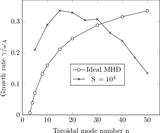
Figure 3: Linear growth rate for simulations with $\omega_{*}$ and $S=10^{4}$

High resistivity results in an increase in growth-rate above the ideal MHD case (open circles), whilst high-$n$ modes are suppressed by diamagnetic drift effects in line with theoretical expectations. The peak growth-rate now occurs at $n=15$, and so this toroidal mode-number is used as a starting point for the nonlinear results shown in figure 4.

(a) Plasma displacement at the outboard mid-plane outwards (solid) and inwards (dashed)

(b) Surface-averaged pressure profiles

(c) Plasma energy loss $\Delta W_{ped}/W_{ped}$

Figure 4: Nonlinear simulation results with $\omega_{*}$ and $S=10^{4}$

Figure 4(a) shows the plasma displacement, measured by finding where the pressure crosses a threshold. Outwards displacement is shown as a solid line, and inwards displacement as a dashed line: These are approximately equal in the linear regime (as expected since mode goes like $\exp\left(in\zeta\right)$ ), but begin to diverge once the displacement exceeds $\sim 1-2$cm with the outgoing filament growth-rate reducing whilst the ingoing hole continues to grow at the linear rate.

Figure 4(b) shows the pressure profiles averaged over (equilibrium) flux surfaces at the times indicated by vertical lines in figure 4(a). This shows that this eruption propagates far into the plasma beyond the steep pressure-gradient region (shown in the $t=0$ equilibrium profile in figure 4(b), and in figure 1(a)).

To quantify the size of the ELM eruption, and provide a measure which can be compared against typical experimentally measured ELM sizes, the thermal energy from the inner edge of the domain ($R=4.2$m at the outboard mid-plane) to $R=4.6$m (vertical line in figure 4(b)) $W_{ped}=\int 3P/2dV$ is used. The fraction of this energy lost during the ELM crash $\Delta W_{ped}/W_{ped}$ is shown in figure 4(c). For this highly resistive case, approximately $30$% of the thermal energy in the pedestal is lost, limited by the radial size of the computational domain.

7 Diamagnetic and hyper-resistive simulations

Using high resistivities to damp small-scale structures and maintain numerical stability in the nonlinear regime results in greatly increased growth-rates, modified stability thresholds, and large eruptions which propagate far into the plasma.

An alternative effect which damps high-$k$ structures whilst minimising the effect on large-scale structures is hyper-resistivity [29, 35, 36]: The parallel electric field equation for $\psi=A_{||}/B_{0}$ is modified to

$$\frac{\partial\psi}{\partial t}=-\frac{1}{B_{0}}\nabla_{||}\phi+\frac{\eta}{\mu_{0}}\nabla_{\perp}^{2}\psi+\frac{\eta_{H}}{\mu_{0}}\nabla_{\perp}^{4}\psi$$

where $\eta_{H}$ is a hyper-resistivity. The hyper-Lundquist number is then defined analogously to the Lundquist number as the dimensionless ratio of an Alfvén wave crossing time to a hyper-diffusion timescale. $S_{H}=\mu_{0}R_{0}^{3}v_{A}/\eta_{H}=S/\alpha_{H}$. The hyper-Lundquist parameter $\alpha_{H}=\eta_{H}/R^{2}\nu_{ei}$ can be estimated from electron collisional viscosity [29] as $\alpha_{H}\simeq\mu_{e}/R^{2}\nu_{ei}$ if it is assumed that the electron viscosity $\mu_{e}$ is comparable to the anomalous electron thermal diffusivity $\mu_{e}\simeq\chi_{e}\simeq 1$m²/s. Taking a value of $\nu_{ei}\simeq 10^{5}$s^-1 gives $\alpha_{H}\simeq 10^{-4}-10^{-6}$ for $R\simeq 3$m.

Taking $S=10^{8}$ and $S_{H}=10^{12}$, the perpendicular scale-length of the parallel current can be estimated this time by balancing $\partial\psi/\partial t$ against the hyper-resistive term. This gives $\Delta_{H}\simeq R\left(\omega_{A}/\gamma/S_{H}\right)^{1/4}\simeq 2$mm, which is of the order of the radial grid spacing $\Delta_{\psi}\simeq 1.1$mm, and an order of magnitude larger than was the case with only resistivity included. By including this hyper-resistive effect, realistic resistivities of $S\sim 10^{8}$ can be simulated.

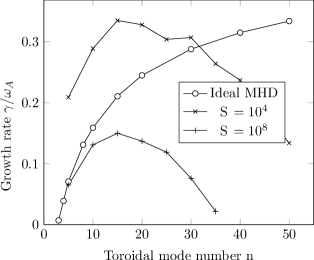
Figure 5: Linear growth rate for simulations with $\omega_{*}$ and $S_{H}=10^{12}$

Linear growth-rates are shown in figure 5, with the ideal MHD and resistive (figure 3) results for comparison. Growth-rates are below the ideal MHD case, stabilised at high-$n$ by diamagnetic drifts as expected, and recover the low-$n$ ideal MHD growth-rates. This is encouraging and an improvement on the resistive case where enhanced growth-rates were found.

Nonlinear simulation results are shown in figure 6 using $S=10^{8}$ and $S=10^{12}$, with the same plots as in figure 4.

(a) Plasma displacement at the outboard mid-plane outwards (solid) and inwards (dashed)

(b) Surface-averaged pressure profiles

(c) Plasma energy loss $\Delta W_{ped}/W_{ped}$

Figure 6: Nonlinear simulation results with $\omega_{*}$, $S=10^{8}$ and $S_{H}=10^{12}$

As with the resistive case, figure 6(a) shows that the growth-rate approximately follows the linear growth-rate until a displacement of approximately $1-2$cm (up to $t\simeq 75\tau_{A}$) at which point the growth-rate of the plasma displacement slows and the profiles relax.

A striking difference between this low-resistivity case and the resistive case presented in section 6 is that the eruption no longer penetrates far into the core. Instead, after a fast initial stage the profiles relax on timescales of $10$’s of $\tau_{A}$ as shown in figure 6(b) where the surface-averages pressure profiles are plotted for the times indicated as vertical lines in figure 6(a).

The ELM loss $\Delta W_{ped}/W_{ped}$ is plotted as a function of time in figure 6 which shows a loss of $\sim 6$% of the pedestal thermal energy (with a continuing slow relaxation of the profiles). Most of this is due to convective losses in the initial fast stage of the eruption as filaments are ejected from the plasma. Note that the simplified model used here does not include parallel heat conduction, and so only convective losses are captured. Convective losses are thought to be important in x-point simulations where open field-lines can quickly transport away heat, but will probably not play such a key role in these circular “limiter” plasmas without open field-lines.

8 Effect of resistivity on ELM size

The size of the ELM eruption varies dramatically between the high and low resistivity cases (figure 4 and 6 respectively). The transition between these cases is shown in figure 7 which plots the ELM loss fraction $\Delta W_{ped}/W_{ped}$ as a function of the Lundquist number for a fixed $S_{H}=10^{12}$.

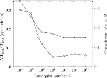
Figure 7: ELM size against Lundquist number for fixed $S_{H}=10^{12}$

As the Lundquist number is increased, the loss of thermal energy during the ELM (open circles in figure 7) is seen to drop from $\sim 30$% to $\sim 6$% over a range of $S=10^{5}-10^{7}$. One explanation for the more violent eruptions at high resistivity is the increased linear growth-rate: Also plotted in figure 7 (crosses) is the linear growth-rate of the $n=15$ mode, which also shows an increase over a similar range of Lundquist number.

Since there is little change in the linear growth-rate between $S=10^{6}$ and $S=10^{7}$, whilst ELM size changes by a factor of $\sim 2$, the process which determines ELM loss may be a nonlinear phenomenon related to dissipation at the smallest scales. The point at which the resistivity starts to dominate over the hyper-resistivity ($\Delta_{R}=\Delta_{H}$) is given by $S=\sqrt{S_{H}\omega_{A}/\gamma}\sim 2\times 10^{6}$. Increasing the Lundquist number above $10^{6}$ therefore has little effect on the ELM size $\Delta W_{ped}/W_{ped}$ because hyper-resistivity is the dominant dissipative effect. This may then imply that in high Lundquist number regimes relevant to high-performance discharges, the (convective) ELM loss is determined by the hyper-resistive dissipation rather than the resistivity.

9 Magnetic field structure

In order to understand the ELM eruption in the low resistivity case (figure 6), Poincaré (puncture) plots of the magnetic field structure have been produced and compared against the pressure contours. Figure 8 shows the (normalised) pressure $2\mu_{0}p/B^{2}$ at the outboard mid-plane as a function of $\psi$ and toroidal angle $\zeta$ for $t=60\tau_{A}$ and $t=70\tau_{A}$. On top of these are plotted a puncture plot of the magnetic field showing the field structure at these two times.

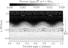
(a) $t=60\tau_{A}$

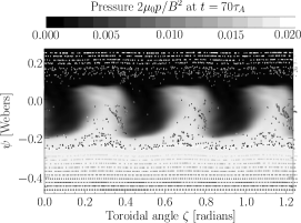
(b) $t=70\tau_{A}$

Figure 8: Pressure and magnetic field puncture plot at outboard mid-plane. Minor radius increases going up the figures

Up to $t\sim 60-65\tau_{A}$, the magnetic field surfaces follow pressure isosurfaces (frozen-in condition), and the growth-rate remains approximately the same as the linear mode (figure 6(a)). During this period, the leading edge of the erupting filaments steepens. This forces flux-surfaces closer together at the tips of the filaments, reducing perpendicular scale lengths and increasing the importance of (hyper-)resistivity. Eventually, the flux-surfaces break and the magnetic field becomes disordered. After this time ($t\simeq 65\tau_{A}$), the eruption growth-rate falls and the profiles begin to relax on a slower timescale.

10 Conclusions

Simulations of Edge Localised Modes (ELMs) have been performed using the BOUT++ simulation code [28] for a shifted circle equilibrium (cbm18_dens8). The linear structure and growth-rates of the unstable ballooning modes have been benchmarked without diamagnetic effects against the linear ideal MHD codes ELITE and GATO showing good agreement. By incorporating diamagnetic drift and hyper-resistivity, the scale length of $J_{||}$ structures can be resolved, allowing nonlinear simulations with resistivities relevant to high-performance H-mode tokamak edge plasmas. These show reasonable ELM losses of $\sim 6$% of the pedestal thermal energy, with a limited radial extent, in contrast to simulations with enhanced resistivities.

Results at high Lundquist number indicate that eruptions consist of two stages: a fast emergence of plasma “fingers” at approximately the linear growth-rate (figure 6(a)), during which time the frozen-in condition is obeyed (figure 8(a)). This eruption results in a steepening of the pressure profile at the tips of the plasma fingers, forcing flux surfaces closer together and steepening local pressure gradients. Once the fingers have emerged $\sim 1-2$cm, reconnection occurs at these high-gradient regions, the growth-rate is reduced and filaments begin to break up as the plasma profiles relax (figure 6(b)).

Experimentally, it is found that the ELM size $\Delta W_{ped}/W_{ped}$ decreases as collisionality $\nu^{*}$ is increased [2, 37]. The results presented in figure 7 indicate the opposite trend at low Lundquist numbers, with the size of ELM eruptions increasing with collisionality given the same starting pressure and $J_{||}$ profiles. At high Lundquist numbers (i.e. low $\nu^{*}$) relevant to H-mode pedestals, ELM size has been found to be quite insensitive to Lundquist number, with dissipation dominated by hyper-resistivity. The variation of hyper-resistivity with collisionality is however not well known. Assuming a constant electron viscosity $\mu_{e}\sim 1$m²/s gives $\alpha_{H}\propto 1/\nu$, and so $S_{H}\sim const$ (since $S\propto 1/\nu$). This may imply that convective ELM losses are approximately constant with collisionality, and that the observed variation of ELM loss with $\nu^{*}$ is due to another process such as increasing parallel conductive losses at low collisionality.

A important consideration when interpreting the results presented here is that in these simulations, variation in H-mode pedestal characteristics or bootstrap current with collisionality has not been included, though in practice all these things would vary and change the point at which an ELM is triggered. Predictions of ELM size in future devices depends on a model of the H-mode pedestal from which to start a nonlinear ELM simulation, either coupling kinetic and fluid models such as work coupling XGC0 to M3D [38]. Other possibilities include using a semi-heuristic model such as EPED1 [39] to provide input to a starting equilibrium.

Further work includes the incorporation of parallel heat conduction effects in order to study the conductive losses in conjunction with the convective losses studied here. As mentioned in section 6, non-linear generation of poloidal flows have been found to be important in breaking off ELM filaments [20, 21] and so incorporation of these effects into BOUT++ simulations is a priority.

References

References

- [1] M Keilhacker, F Becker, K Bernhardi, et al. Plasma Phys. Control. Fusion, 26:49, 1984.
- [2] E J Doyle et al. In 22nd IAEA Fusion Energy Conference, 2008.
- [3] P B Snyder et al. Physics of Plasmas, 9:2037, 2002.
- [4] H R Wilson et al. Physics of Plasmas, 9:1277, April 2002.
- [5] L C Bernard, F J Helton, and R W Moore. Comp. Phys. Comm., 24(3-4):377–380, 1981.
- [6] A B Mikhailovskii et al. Plasma Phys. Rep., 23:844, 1997.
- [7] I T Chapman et al. Physics of Plasmas, 13:062511, 2006.
- [8] C C Hegna, J W Connor, R J Hastie, and H R Wilson. Physics of Plasmas, 3:584, 1996.
- [9] J W Connor, R J Hastie, H R Wilson, and R L Miller. Physics of Plasmas, 5:2687, 1998.
- [10] H R Wilson and S C Cowley. Phys. Rev. Lett., 92:175006, 2004.
- [11] P Zhu, C C Hegna, and C R Sovinec. Physics of Plasmas, 13:102307, 2006.
- [12] P Zhu et al. Physics of Plasmas, 14:055903, 2007.
- [13] C R Sovinec et al. J. Comput. Phys., 195:355–386, 2004.
- [14] D P Brennan et al. Journal of Physics: Conference Series, 46:63–72, 2006.
- [15] A Y Pankin et al. Plasma Phys. Control. Fusion, 49:S63–S75, 2007.
- [16] B J Burke et al. Physics of Plasmas, 17:032103, 2010.
- [17] P B Snyder, H R Wilson, and X Q Xu. Physics of Plasmas, 12:056115, May 2005.
- [18] P B Snyder, H R Wilson, and X Q Xu. In Fluid Modelling of ELMs, Boulder, CO, 2006.
- [19] G T A Huysmans and O Czarny. Nucl. Fusion, 47:659–666, 2007.
- [20] G T A Huysmans et al. Plasma Phys. Control. Fusion, 51:124012, 2009.
- [21] S Pamela, G Huysmans, and S Benkadda. Plasma Phys. Control. Fusion, 52:075006, 2010.
- [22] B Scott. Physics of Plasmas, 12:102307, 2005.
- [23] B Scott. Plasma Phys. Control. Fusion, 48:A387, 2006.
- [24] W Park et al. Physics of Plasmas, 6:1796, 1999.
- [25] L E Sugiyama et al. APS Meeting, October 2006.
- [26] L E Sugiyama and the M3D team. J. Phys.: Conf. Ser., 180:012060, 2009.
- [27] N M Ferraro et al. In 51st APS meeting, November 2009.
- [28] B D Dudson et al. Comp. Phys. Comm., 180:1467–1480, 2009.
- [29] X Q Xu et al. Submitted to Phys. Rev. Lett., 2010.
- [30] R D Hazeltine and J D Meiss. Plasma Confinement. Dover publications, 2003.
- [31] A M Dimits. Phys. Rev. E, 48(5):4070–4079, Nov 1993.
- [32] B D Scott. New J. Physics, 4:52.1–52.30, July 2002.
- [33] A Bondeson, G Vlad, and H Lutjens. Phys. Fluids B, 4:1889, 1992.
- [34] H R Strauss et al. Physics of Plasmas, 2:1229, 1995.
- [35] P K Kaw et al. Phys. Rev. Lett., 43:1398, 1979.
- [36] S E Caunt and M J Korpi. A & A, 369:706–728, 2001. arXiv:astro-ph/0102068.
- [37] A Loarte et al. Plasma Phys. Control. Fusion, 45:154969, 2003.
- [38] G Park et al. Journal of Physics: Conference Series, 78:012087, 2007.
- [39] P B Snyder et al. Nucl. Fusion, 49:085035, 2009.