Elastic Energy and Phase Structure in a Continuous Spin Ising Chain
with Applications to the Protein Folding Problem

Abstract

We present a numerical Monte Carlo analysis of a continuos spin Ising chain that can describe the statistical proterties of folded proteins. We find that depending on the value of the Metropolis temperature, the model displays the three known nontrivial phases of polymers: At low temperatures the model is in a collapsed phase, at medium temperatures it is in a random walk phase, and at high temperatures it enters the self-avoiding random walk phase. By investigating the temperature dependence of the specific energy we confirm that the transition between the collapsed phase and the random walk phase is a phase transition, while the random walk phase and self-avoiding random walk phase are separated from each other by a cross-over transition. We also compare the predictions of the model to a phenomenological elastic energy formula, proposed by Huang and Lei to describe folded proteins.

I Introduction

The concept of universality wilson , kadanoff divides critical physical systems into universality classes that differ from each other essentially only by their space-time dimensionality and the symmetry group of their order parameter. This enables the computation of critical properties for an entire class of physical systems using only a single representative model. In the case of polymers one expects that there are three different nontrivial phases and these correspond to the universality class of self-avoiding random walk (SARW), to the universality class of Brownian motion i.e. ordinary random walk (RW), and to the universality class of polymer collapse degennes1 . These phases are each characterized by the different values of certain critical exponents that describe the scaling properties of the polymer in the limit where the number $N$ of monomers becomes large. The most widely used critical exponent, the compactness index $\nu$, computes the inverse of the Hausdorff dimension of the polymer. It can be introduced by considering how the polymer’s radius of gyration $R_{g}$ increases in the number of monomers, asymptotically for large values of $N$ macro ,

$$R^{2}_{g}\ =\ \frac{1}{2N^{2}}\sum_{i,j}({\bf r}_{i}-{\bf r}_{j})^{2}\ \approx\ R_{0}^{2}N^{2\nu}(1+\beta_{1}N^{-\Delta_{1}}+...)$$ (1)

Here ${\bf r}_{i}$ ($i=1,2,...,N$) are the locations of the $N$ monomers in $\mathbb{R}^{3}$. The critical exponents $\nu$ and $\Delta_{1}$ are universal quantities. But the form factor $R_{0}$ that characterizes the effective distance between the monomers in the large $N$ limit, and the amplitude $\beta_{1}$ that parametrizes the leading finite size corrections, are not. The asymptotic expansion (1) is an example of a general result wegner , sokal that states, that when $N$ becomes large the mean value of any global observable $\mathcal{O}$ of a polymer should behave like

$$<{\mathcal{O}}>_{N}\ =\ AN^{p}\left[1+\frac{\alpha_{1}}{N}+\frac{\alpha_{2}}{N^{2}}+\dots\right.$$

$$\left.+\frac{\beta_{1}}{N^{\Delta_{1}}}+\frac{\beta_{2}}{N^{\Delta_{1}+1}}+\frac{\beta_{3}}{N^{\Delta_{1}+2}}+\dots\right]$$ (2)

where the exponents are universal, but the pre-factor and the various amplitudes are all non-universal.

For a polymer the compactness index has the following mean field (mf) values degennes1 :

$$\nu_{\rm mf}\ =\ \left\{\!\!\!\!\begin{matrix}3/5\ \ {\rm SARW}\\ \!\!\!1/2\ \ \ \ {\rm RW}\\ \ \ \ \ 1/3\ \ {\rm collapsed}\end{matrix}\right.$$ (3)

As a function of temperature, the collapsed phase occurs at low temperatures (bad solvent) while the SARW describes the high temperature (good solvent) behavior of polymers. The random walk phase takes place at the $\Theta$-temperature that separates the SARW phase from the collapsed phase. In general the mean field values of the critical exponents acquire corrections due to fluctuations, and for the universality class of the self-avoiding random walk the improved values are $\nu=0.5880\pm 0.0015$ and $\Delta_{1}=0.47\pm 0.03$. These values were obtained in Zinn by utilizing the concept of universality that relates the self-avoiding random walk with the $n\to 0$ component $\phi^{4}$ field theory degennes2 . The subsequent direct Monte Carlo evaluation reported in sokal gave the very similar values $\nu=0.5877\pm 0.0006$ and $\Delta_{1}=0.56\pm 0.03$, in line with the concept of universality.

Qualitatively, at the level of a mean field theory the phase structure of a polymer can be described in terms of the Flory-Huggins theory degennes1 . For this we characterize the polymer concentration by an order parameter $\phi(x)$, with $0\leq\phi(x)\leq 1$. At low concentrations the polymer free energy density (per temperature) has the Landau expansion

$$\frac{1}{T}E[\phi]=\eta(\nabla\phi)^{2}+\gamma\cdot\phi\ln\phi+\frac{1}{2}(1-2\chi)\phi^{2}+\frac{g}{3!}\phi^{3}+...$$ (4)

Here $\eta,\gamma,\chi$ and $g$ are parameters. The first term is a stiffness term. The second term describes entropy contrubutions. The third term describes monomer-monomer interactions; the (Flory) interaction parameter $\chi$ is generically a decreasing function of temperature. The last term characterizes the three-body (and higher order contributions) monomer interactions. The phase structure can be exposed by by ignoring the stiffness term and by minimizing the remaining potential energy contribution to free energy. With proper relative values of the parameters the potential has a form that is familiar from spontaneous symmetry breaking: When the ground state expectation value $<\!\!\phi\!\!>$ is non-vanishing we are in the collapsed phase while the vanishing value $<\!\!\phi\!\!>\approx 0$ implies that we are in the universality class of self-avoiding random walk. The border line that separates these two phases determines the $\Theta$ temperature where the polymer is in the universality class of random walk. It occurs at that value of temperature (or denaturant concentration) for which the excluded volume parameter vanishes, and to first order

$$1-2\chi(T_{\Theta})\ =\ 0$$

Thus, for $\chi(T)>1/2$ we are in the collapsed phase while for $\chi(T)<1/2$ we enter the SARW phase and in particular at the $\Theta$-point the $\phi^{2}$ (i.e. mass) contribution to the free energy is absent.

Here we shall present results of an extensive numerical analysis of the polymer phase structure. Our approach is based on the chiral homopolymer model introduced in ulf . The applicability of the model to analyze the properties of chiral polymers in all three phases can be justified by the concept of universality. Indeed, the derivation of the model in ulf is very much based on the universality concept: The model accounts for the monomer complexity, the presence of amino acid side chains in proteins, and polymer-solvant interactions in an effective manner. In particular, the model appears to describe certain universal properties of the folded proteins dill in the Protein Data Bank (PDB) pdb with a very high accuracy. More recently, it has also been shown maxim , nora that the model supports dark solitons and the presence of these solitons appears to be related to the emergence of the collapsed phase. These solitons can also describe folded proteins in PDB with a subatomic accuracy of less than 1 Ȧngström in root mean square distance (RMSD). This also motivates us to compare our results to a recently presented phenomenological model of protein folding huang1 .

II The Model

The model introduced in ulf is defined by the following internal energy,

$$E = \phantom{+}\underset{ij}{\sum}a_{ij}\left\{1-\cos\left[\omega_{ij}\left(\kappa_{i}-\kappa_{j}\right)\right]\right\}$$

$$+\underset{i}{\sum}\left\{b_{i}\kappa_{i}^{2}\tau_{i}^{2}+c_{i}\left(\kappa_{i}^{2}-m_{i}^{2}\right)^{2}+d_{i}\tau_{i}\right\}$$

Here $i,j=1,...,N$ label the $N$ monomers of a (chiral) polygonal chain in $\mathbb{R}^{3}$. These monomers are located at the vertices of the polygon, and the chain geometry changes when the polymer fluctuates in $\mathbb{R}^{3}$. The geometry is determined by the order parameter $\kappa_{i}$ that is a discrete lattice version of the Frenet curvature, and by the order parameter $\tau_{i}$ that is the lattice version of the Frenet torsion ulf . Once the values of $(\kappa_{i},\tau_{i})$ for each $i=1,...,N$ are given the actual shape of the polymer as a polygonal chain in the three dimensional space can be computed by integrating the appropriate discrete version of the Frenet equations. This integration introduces parameters $\delta_{i}$, the three dimensional distances between the monomers.

The $a_{ij},\omega_{ij},b_{i},...,d_{i}$ in (II) are parameters. The first sum in the free energy describes long-distance interactions, we have introduced the cosine function to tame excessive fluctuations in $\kappa_{i}$ in the numerical simulations. In the second sum the first term describes the interaction between $\kappa_{i}$ and $\tau_{i}$, and the second term describes the self-interaction of $\kappa_{i}$. Finally, the last term is a discretized version of the one dimensional Chern-Simons functional, it is the origin of chirality in the polymer chain ulf , with handedness that depends on the sign of $d_{i}$.

For a general polymer the quantities ($a_{ij},\omega_{ij},b_{i},c_{i},$ $\mu_{i},d_{i}$) are a priori site-dependent parameters, and different values of these parameters can be used to describe different kind of monomer (amino acid) structures. For generic $a_{ij}$ (II) is a spin-class model. Here we shall be interested in the limiting case of a homopolymer where we restrict ourselves to only the nearest neighbor interactions with

$$a_{ij}=\left\{\begin{matrix}\hskip-34.14322pta\cdot(\delta_{i,i+1}+\delta_{i,i-1})\ \ \ \ (i=2,...,N-1)\\ \hskip 5.69046pta\ \ \ \ \ \ \ \ (i=1,j=2)\ \ \&\ \ (i=N-1,j=N)\end{matrix}\right.$$ (6)

and we also select all the remaining parameters to be independent of the site index $i$. Thus the model in the form studied here reads

$$E=\phantom{+}\underset{n.n.}{\sum}a\left\{1-\cos\left[\omega\left(\kappa_{i}-\kappa_{j}\right)\right]\right\}$$

$$+\underset{i}{\sum}\left\{b\kappa_{i}^{2}\tau_{i}^{2}+c\left(\kappa_{i}^{2}-m^{2}\right)^{2}+d\tau_{i}\right\}$$ (7)

where the first sum extends over the nearest neighbors; Notice that since the overall scale of the parameters $a,b,c$ and $d$ can be absorbed into the definition of the scale of the Metropolis temperature $T$, as it stands there are five independent intrinsic parameters. Consequently the scale of energy, say in electronvolts, remains indeterminate and should be defined by (re)normalization at some convenient value of $T$. We also note that classically, the model (7) has a ground state which is a helix, with $\kappa_{i}\approx\pm m$.

We select the numerical values of the parameters in a manner that allows for a direct statistical comparison to PDB data. These values have been found by a trial-and-error comparison with PDB data ulf and they are shown in Table 1.

Parameter	Value
$a$	4
$\omega$	4.25
$b$	$5.488\cdot 10^{-4}$
$c$	0.5
$m$	24.7
$d$	-20

Table 1: Parameter values of the model (II) that we use in our simulations

.

Furthermore, we shall assume that the distances $\delta_{i}$ between the monomers that we need to introduce when we integrate the discrete Frenet equations to construct the polygonal chain in $\mathbb{R}^{3}$, have the fixed value

$$|{\bf r}_{i}-{\bf r}_{i-1}|=\delta\ =\ 3.8\ ({\buildrel{}_{\circ}\over{\mathrm{A}}})\ \ \ \ i=2,...,N.$$ (8)

This value (in ${\buildrel{}_{\circ}\over{\mathrm{A}}}$) is chosen to coincide with the average distance between $C_{\alpha}$ carbons in the backbone of PDB proteins. Finally, we exclude steric clashes by demanding that the distance between any two monomers satisfies the bound

$$|{\bf r}_{i}-{\bf r}_{j}|\geq z\ =\ 3.7\ ({\buildrel{}_{\circ}\over{\mathrm{A}}})\ \ \ {\rm for}\ \ \ |i-j|\geq 2.$$ (9)

Again, this numerical value has been chosen to match the protein data in PDB.

We have used the standard Metropolis algorithm to simulate the model (II). The initial configuration is a straight rod with $\kappa_{i}=\tau_{i}=0$. Each Monte-Carlo step consists of a shift of the curvature and torsion by a typical value of $\Delta\kappa_{i}=\Delta\tau_{i}=0.05$. This shift is accepted with the probability

$$P=\min\left(1,\exp\left(-\frac{\triangle E}{T}\right)\right)$$

where $T$ is the Metropolis temperature. We use this temperature as an external parameter that allows us to probe the different phases of the polymer.

The simulations proceeded as follows: For each temperature value, between 10 and 16 different polymer lengths was selected. The number of the Monte-Carlo iterations of each chain was chosen to be 11.000 multiplied by the number $N$ of monomers in the polymer. We created around 200 or more polymers for each individual temperature value $T$ and monomer number $N,$ with less for the extremely long and the highest temperature curves. The shortest polymers in our simulations had 50 monomers, and the longest ones had 1.800 monomers. These values were chosen to be representative of the single domain proteins in PDB.

Finally, since the free energy (II), (7) is quadratic in $\tau_{i}$ and furthermore since $\tau_{i}$ only interacts locally, we can eliminate it by using its equation of motion

$$\frac{\partial E}{\partial\tau_{i}}\ =\ 2b_{i}\kappa_{i}^{2}\tau_{i}+d_{i}\ =\ 0$$

$$\Rightarrow\ \ \tau_{i}[\kappa_{i}]=-\frac{d_{i}}{2b_{i}\kappa_{i}^{2}}\ \ \$$ (10)

This gives us

$$E = \phantom{+}\underset{i,j}{\sum}a_{ij}\left\{1-\cos\left[\omega_{ij}\left(\kappa_{i}-\kappa_{j}\right)\right]\right\}$$

$$+\underset{i}{\sum}\left\{c_{i}\left(\kappa_{i}^{2}-m_{i}^{2}\right)^{2}\ -\frac{d_{i}^{2}}{2b_{i}\kappa_{i}^{2}}\right\}$$

and in the limit of uniform chain and small $\omega$ we get (after we add boundary contributions and choose $\kappa_{0}=\kappa_{N+1}=0$)

$$E\ \approx\ -a\omega^{2}\sum\limits_{i}\kappa_{i}\kappa_{i+1}\ +$$

$$+\sum\limits_{i}\left\{a\omega^{2}\kappa_{i}^{2}+c\left(\kappa_{i}^{2}-m^{2}\right)^{2}\ -\frac{d^{2}}{4b\kappa_{i}^{2}}\right\}$$ (11)

We recognize here a version of the continuos spin Ising chain ising : Indeed, the only difference between (11) and the conventional continuous spin Ising chain is in the presence of the last term in (11). We note that this last term that has its origin in (10), is quite reminiscent of the potential term that appears in the widely studied Calogero model galo , for the relative coordinate in the two-body case. Furthermore, if we absorb the parameter combination $a\omega^{2}$ into the definition of overall scale of temperature , in (10), (11) there are only four independent parameter combinations.

It has been a commonly held point of view barma that the lattice version of the $\phi^{4}$ model is always in the same universality class with the pure Ising model. But this has been disputed in the one dimensional case by explicit computations e.g. in baker . Here we have an additional interaction term, the last Calogero-type term in (11), and we shall explicitely show that the ensuing phase structure is highly nontrivial.

III The radius of gyration

We shall first investigate the radius of gyration (1) with the goal to confirm that the model ulf does indeed describe the three different polymer phases characterized by the mean field values (3) of the critical exponent $\nu$.

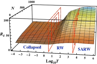
Figure 1: The radius of $R_{g}$ as a function of temperature $T$ and the number of monomers $N$. The three putative phases are identified with the putative position of the ensuing critical temperatures, denoted by the vertical planes.

In Figure 1 we show how the radius of gyration $R_{g}$ depends on the (Metropolis) temperature $T$ and the number of monomers $N$. In Figure 2 we depict the $T$ dependence of $\nu$,

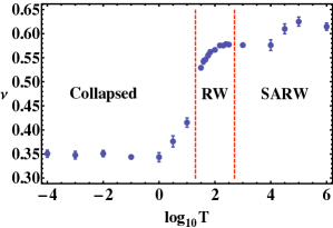
Figure 2: The compactness index $\nu$ vs. temperature $T$. The vertical lines correspond to temperature values where $\nu(T)$ reaches the mean field values (3).

and figure 3 shows the $T$ dependence of the pre-factor $R_{0}$ in (1).

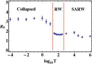
Figure 3: The pre-factor $R_{0}$ in (1) vs. temperature $T$. The vertical lines correspond to the temperature values where $\nu(T)$ in figure 2 reaches the mean field values (3).

III.1 Collapsed phase

In the figure 1 we clearly identify a low-temperature phase which is the putative collapsed phase. In this phase $R_{g}$ is constant, or has only very weak $T$ dependence, and we can fit the data with very high accuracy using the following relation,

$$R_{g}=R_{0}N^{\nu}\,,$$ (12)

where $R_{0}$ and $\nu$ are the fitting parameters. From the data in figure 2 we estimate in the low temperature limit

$$\nu\ =\ 0.348\pm 0.007$$ (13)

This is so close to the mean field value $\nu=1/3$ of the collapsed phase, that obviously we are in that phase.

The parameter $R_{0}$ that we present in Fig. 3 describes the effective distance between the monomers. In the collapsed phase we estimate in the low temperature limit

$$R_{0}\ =\ 3.25\pm 0.15\ \ ({\buildrel{}_{\circ}\over{\mathrm{A}}})$$

This is clearly smaller than the bare value (8) in our model, proposing that in the collapsed phase the monomers have the tendency to become more densely packed also along the polymer chain.

From our data we are not able to deduct any non-vanishing value for the sub-leading critical exponent $\Delta_{1}$ in (1).

When the temperature increases beyond $\log_{10}T\approx 0$, $\nu(T)$ starts increasing and we enter a transition region between the collapsed phase and the putative random walk phase. At the same time as the value of $\nu$ starts increasing, the value of $R_{0}$ decreases and when temperature approaches the value foot1

$$T_{PDB}\ \approx\ 3.81\pm 1.52$$ (14)

we obtain the fit

$$R_{g}\ \approx\ 2.8\,\cdot N^{0.38}$$ (15)

for $50\leq N\leq 1.800$ which is very close to the estimate ulf

$${R_{g}}^{\hskip-4.26773ptPDB}\ \approx\ 2.25\,\cdot N^{0.38}$$ (16)

that describes the dependence of the radius of gyration on the number $N$ of $C_{\alpha}$ carbons for all single strand proteins in PDB with $75<N<1.000$. This suggests that the model probably gives its best approximation to the PDB data in its collapsed phase, near the transition to the random walk phase. However, we point out that when $T\approx T_{PDB}$ both $\nu(T)$ and $R_{0}(T)$ have a quite strong temperature dependence, indicative of vicinity of a phase transition that makes the accuracy of our estimates prone to relatively large errors, and for more precise estimates one needs simulations with substantially more computer time.

III.2 RW and SARW phases

In Figure 4 we display how the radius of gyration depends on the number of monomers $N$ for a range of values of temperature beyond the collapsed phase, and compare the data with a fit of the form (12). As visible in this figure, even beyond the collapsed phase the data can be fitted with very high accuracy by the relation (12). However, unlike in the collapsed phase where the radius of gyration is practically temperature independent, both in the putative random walk phase and in the putative self-avoiding random walk phase the radius of gyration is a slowly but monotonically increasing function of the temperature.

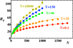
Figure 4: The radius of gyration $R_{g}$ vs. the number of monomers $N$ at different values of temperature $T$. The error bars are of the same order or smaller than the size of the symbols used. The dashed lines represent the fits by equation (12).

The transition from the collapsed phase to the putative random walk phase is very visible in our figures 2 and 3. There is a clear, rapid transition in both $\nu(T)$ and $R_{0}(T)$, reminiscent of a phase transition. From figure 2 we estimate that at the transition point $\nu$ is very close to the value

$$\nu\approx\frac{1}{2}$$

which is the mean field value for the $\Theta$-point. For $T>T_{\Theta}$, the compactness index $\nu(T)$ is a slowly increasing function of temperature that eventually plateaus around the value

$$\nu\approx 0.58$$

This is slightly above the $\Theta$-point value, but slightly below the SARW values reported in Zinn , sokal . Since the compactness index $\nu(N)$ appears to have a tendency to approach its large-$N$ limit from above sokal , we conclude that we are in the RW phase.

For the effective monomer distance $R_{0}$ we find the value

$$R_{0}\ =\ 1.67\pm 0.03\ \ (\dot{A})$$

which is clearly lower than the bare value (8).

In general one expects that the transition between the collapsed phase and the RW phase is a phase transition, while the transition between the RW and SARW phases is a smooth cross-over degennes1 . The results in figures 1-3 are in line with this, the transition between the RW phase and the putative self-avoiding random walk phase is much less dramatic than the transition between the collapsed phase and the RW phase. This also makes the precise identification of the RW and SARW phases more involved:

We find that asymptotically at very high temperatures $\nu$ approaches the value

$$\nu{\buildrel{}_{T\to\infty}\over{\longrightarrow}}\ 0.62\pm 0.03$$

This is slightly above the mean field value and the final values obtained in Zinn , sokal , but fully in line with the computations in sokal that revealed that the asymptotic value of $\nu$ is reached from above as the number of monomers increases; We note that here we have restricted ourselves to consider only values of $N$ in the range $50-1.000$ that are relevant for single strand proteins, while sokal considered self-avoiding walks with up to 80.000 steps. Consequently finite scaling corrections have a much stronger effect on our estimates. We also point out that as $T\to\infty$ only the self-avoiding condition (9) persists. Thus, in this limit we must be in the universality class of SARW.

We note that for the effective monomer distance $R_{0}$ we find in the high temperature limit the value

$$R_{0}\ =\ 1.62\pm 0.08\ \ (\dot{A})$$

that is, essentially the same as in the RW phase.

In summary, the distinction between the collapsed phase and the RW phase appears very clear in our analysis of the compactness index, and suggests the presence of either a first or a second order phase transition. On the other hand, the transition from RW phase to SARW phase is much more difficult to pinpoint, and it appears to proceed much more like a smooth cross-over transition than a phase transition. These observations are fully in line with general expectations degennes1 , and we conclude that the model ulf does indeed correctly describe all the three phases of a polymer.

IV Elastic Energy

IV.1 General behavior

For the fixed parameter values that we have given in table 1 the free energy (7) is a function of two extrinsic parameters, the temperature $T$ and the number of monomers $N$. Its numerical value can be identified as the elastic energy of the polymer chain. In figure 5 we display a three dimensional plot of (a logarithm of) the specific elastic energy i.e. the elastic energy per monomer as a function of these two parameters

$$E_{specific}=\frac{E}{N}$$ (17)

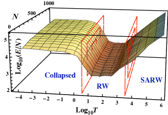
Figure 5: A three dimensional plot of a logarithm of the specific energy as a function of a logarithm of temperature $T$ and the number of monomers $N$. The three phases are identified and the putative position of the ensuing critical temperatures are denoted by the vertical planes.

In this figure we clearly identify the presence of three different phases that are separated from each other by clearly identifiable transition (critical) temperatures $T_{c1}$ and $T_{c2}$ (with $T_{c1}<T_{c2}$), and both the low temperature collapsed phase ($T<T_{c1}$) and the medium temperature RW phase ($T_{c1}<T<T_{c2}$) are characterized by essentially temperature independent specific energy. Notice that in the collapsed phase the specific energy has a value that is more than one order of magnitude larger than in the RW phase. This is understandable, as it should indeed take much more energy to extend a polymer that is collapsed and resists being extended, than a polymer that behaves like an ideal chain and thus does not really care about its shape. The increase of temperature beyond $T_{c2}$ leads to a transition to the SARW phase, which is characterized by a power-law increase of the specific energy as a function of the temperature: The larger its thermal fluctuations, the more the polymer resists to become extended. Note also that in the collapsed and RW phases the specific energy in figure 5 exhibits a weak dependence on the number of monomers $N$. But in the high temperature SARW phase the specific energy becomes essentially independent of $N$. This is consistent with the expected behavior of self-avoiding random walk, it is driven solely by the condition (9) and no reference to the details of the free energy survives the infinite temperature limit. In this limit, the polymer is only subject to random thermal fluctuations.

IV.2 Critical temperature

We have found that the dependence of the specific energy on temperature displayed in figure 5 can be approximated with a very good accuracy by a function

$$\log_{10}(E/N)=F^{\mathrm{fit}}(\log_{10}T)$$ (18)

that has the following explicit form

$$F^{\mathrm{fit}}(x) = h_{1}+h_{2}\arctan[h_{3}(x-x_{1})]$$ (19)

$$+h_{4}x\,\arctan[h_{5}(x-x_{2})]-h_{6}x\,.$$

The parameters $h_{1}\dots h_{6}$ and $x_{1,2}$ are determined by fitting to the numerical data at fixed value of the monomer number $N$. This explicit form yields an excellent fit whenever there are more than around $N=100$ monomers. In figure 6 we display several examples where we have fitted the functional form (18), (19) to polymers as described by our model, where the values of $N$ are between $200$ and $1.000$.

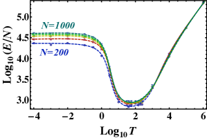
Figure 6: The approximations (dashed lines) of the calculated numerical values (dots) of the specific energy by the function (18), (19) when $N=200,\,400,\,600,\,800,\,1000$. The specific energy is a monotonically rising function of the monomer number. The lowest and the highest sets correspond to $N=200$ and $N=1000$, respectively.

The fitted functional form (18), (19) allows us to pinpoint the two critical temperatures $T_{c1}$ and $T_{c2}$. For this we locate the maxima of the squared logarithmic derivative of the specific energy with respect to the logarithm of temperature,

$$D_{E}(T,N)=\Biggl{[}\frac{\partial\log_{10}E(T,N)}{\partial\log_{10}T}\Biggr{]}^{2}\,.$$ (20)

This quantity resembles susceptibility that is known to have its maxima at the location of critical temperature(s). The result is shown in figure 7.

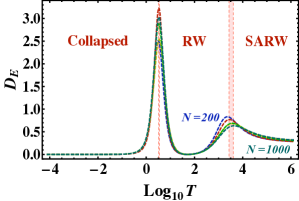
Figure 7: The quantity (20) obtained from the best fits of the functions (18) and (19) for various values of monomer length $N$. The vertical red lines correspond to the critical temperatures (21) and (22). The width of the lines gives the uncertainty in the definition of the critical temperatures.

The maxima of (20) appear as peaks that are clearly visible for all values of $N$ that we have studied and displayed in figure 7. From the results in table 2 we estimate that the critical temperatures have the following values,

$$\log_{10}T_{c1}=0.53\pm 0.02\,,\quad\mbox{or}\quad T_{c1}=3.38\pm 15$$ (21)

$$\log_{10}T_{c2}=3.52\pm 0.09\,,\quad\mbox{or}\quad T_{c2}=3306\pm 716\qquad$$ (22)

Notice that the position of the first maximum is practically the same for all values of $N$, but the larger the value of $N$ the higher the height of the maximum. This indicates that the transition between the collapsed phase and the RW phase at $T=T_{c1}$ is indeed phase transition, which is either of the second order or of the first order; Our analysis is not sufficient to determine the order of this transition.

On the other hand, the transition between the RW and SARW phases at $T=T_{c2}$ is likely to be a smooth crossover transition since now both the position of the maximum and its height do not reflect any similar clearly localized profile with increasing values of monomer number $N$.

$N$	$\log_{10}T_{c1}(L)$	$\log_{10}T_{c2}(L)$
200	0.5023	3.365
300	0.5114	3.397
400	0.5229	3.450
500	0.5402	3.599
600	0.5379	3.570
700	0.5671	3.552
800	0.5184	3.563
900	0.5360	3.534
1000	0.5254	3.638
Avr.	0.53(2)	3.52(9)

Table 2: The critical temperatures $T_{c1}$ and $T_{c2}$, determined for each fixed number of monomers $N$. The averaged value is shown in the last row (in the bold face) along with respective errors.

V The phase dependence of the free energy

We have found that in each of the three phases the elastic energy computed from (7) has its distinct, universal dependence on the monomer number $N$, alternatively radius of gyration $R_{g}$.

V.1 Collapsed phase

In the collapsed phase $T<T_{c1}$ the dependence of the free energy on the number of monomers can be described by the following temperature independent, logarithmically corrected linear law:

$$E(N)/E_{0}=C_{\mathrm{Coll}}N\ln\frac{N}{N_{0}^{\mathrm{Coll}}}\,.$$ (23)

Here $E_{0}$ is a parameter that defines the scale of the energy (say) in electronvolts and must be obtained by an independent measurement. We find the presence of the logarithmic correction to scaling - as opposed to the analytic corrections proposed by (2) - to be quite notable: We have made a very detailed analysis of the functional form (23) and the logarithmic correction to scaling is consistently exceeding the accuracy of any power-law alternative.

The parameters $N_{0}^{\mathrm{Coll}}$ and $C_{\mathrm{Coll}}$ can be calculated using a fitting procedure. The results are shown, respectively, in figure 8. The parameter $N_{0}^{\mathrm{Coll}}$ is essentially temperature independent in the low-temperature regime, with value

$$N_{0}^{\mathrm{Coll}}\simeq 22$$

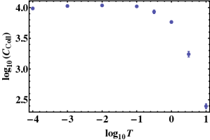
Figure 8: The parameters of the fit (23): $N_{0}^{\mathrm{Coll}}$ (the upper plot) and $C_{\mathrm{Coll}}$ (the lower plot).

In terms of the radius of gyration we get from (12), (13) the approximate expression (per units of energy)

$$E(R_{g})\ \approx\ 971.0\cdot R_{g}^{2.86}\cdot\ln\left[\frac{R_{g}}{9.53}\right]$$ (24)

The relevant aspect of (24) is its dependence on $R_{g}$. Since the radius of gyration scales in proportion to the end-to-end distance the result (24) means there is a very rapidly growing elastic force between the end points of the collapsed polymer in our model, in particular the elastic force is growing clearly more rapidly than in Hooke’s law.

Notice that according to the value of the critical temperature (21), the last data point in Fig. 8 (the one with the highest temperature value) is in the RW phase. However, we have found that the two parameter fit  (23) can still be applied to successfull describe this point.

V.2 RW phase

In the RW phase we have found that the energy obeys the following scaling law (per units of energy)

$$E(T,N)=C_{\mathrm{RW}}(T)N\Biggl{[}1-\left(\frac{N}{N_{0}^{\mathrm{RW}}(T)}\right)^{-\gamma(T)}\Biggr{]}\,.$$ (25)

This is an example of the general form (2). The best fits of the parameters $\gamma$, $N_{0}^{\mathrm{RW}}$ and $C_{\mathrm{RW}}$ are shown in figure 9 as functions of temperature. We find that all of these parameters are essentially temperature independent with the following average central values,

$$\begin{matrix}\gamma&=&0.355(33)\\ N_{0}^{\mathrm{RW}}&=&8.3(1.5)\\ C_{\mathrm{RW}}&=&1098(22)\end{matrix}$$ (26)

These values are shown as horizontal lines in figure 9.

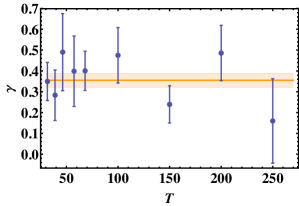
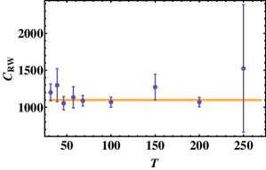
Figure 9: The best fit parameters $\gamma$, $N_{0}^{\mathrm{RW}}$ and $C_{\mathrm{RW}}$ of the function (25). The horizontal lines mark the central values (26), and the width of the lines describe the corresponding errors.

If we use the approximation that $\nu\approx 1/2$ in the RW phase, (26) gives us the Hooke’s law with a (temperature dependent) correction term (per units of energy),

$$E(R_{g},T)\ \approx\ C_{\mathrm{RW}}\left(\frac{R_{g}}{R_{0}}\right)^{2}\Biggl{[}1-(N_{0}^{\mathrm{RW}})^{\gamma}\cdot\ \left(\frac{R_{g}}{R_{0}}\right)^{-2\gamma}\biggr{]}$$ (27)

V.3 SARW phase

In the SARW phase we conclude that the energy is a linear function of the monomer number (per units of energy),

$$E(N,T)=C_{\mathrm{SARW}}(T)N\,.$$ (28)

and with the mean field value of the compactness index $\nu=3/5$ we get in terms of radius of gyration (per units of energy)

$$E(R_{g},T)\ \approx\ C_{\mathrm{SARW}}(T)\left(\frac{R_{g}}{R_{0}}\right)^{5/3}$$ (29)

From our data we are not able to observe any of the correction terms in (2). The only fitting parameter, $C_{\mathrm{SARW}}(T)$, is shown in Fig. (10) as a function of temperature.

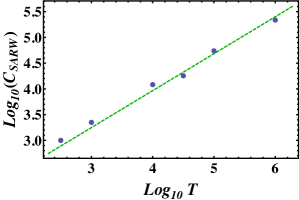
Figure 10: The coefficient of the linear law (28) as a function of temperature. The dashed line illustrates the best fit (30) with the parameters (31).

We also find that the temperature dependence of the coefficient $C_{\mathrm{SARW}}$ can be described by a power law

$$C_{\mathrm{SARW}}(T)=C_{0}\,T^{\alpha}\,,$$ (30)

where the prefactor $C_{0}$ and the exponent $\alpha$ are

$$\begin{matrix}C_{0}&=&12(4)\\ \alpha&=&0.72(6)\end{matrix}$$ (31)

Note that according to the value of the critical temperature (22), in Figure 10 the first two points that have the lowest temperature values belong to the RW phase but they can still be described with the present fit. In fact, the $N$ dependence of the free energy at these two temperature values can be fitted both by the linear law (28) and by the more general power law (25). However, the power-law fit will lead to very large error bars for the best fit parameters, and therefore we have not shown these points in Fig. 9. Moreover, since we expect that the transition between the RW and SARW phases is a crossover, there should be no clear distinction between these phases in the vicinity of the transition region.

The logarithmic (23), power (25) and linear (28) fits are all shown in figure (11).

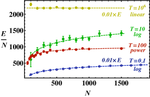
Figure 11: The logarithmic (23), power (25) and linear (28) at various temperatures.

Finally, we summarize the results in Fig. 12 where we show how the specific elastic energy (17) depends on the radius of gyration $R_{g}$ for various temperatures. The upper plot of Fig. 12 corresponds to the collapsed and RW phases. It is very visible that both in the collapsed phase and the RW phase the relation $E_{specific}=E_{specific}(R_{g})$ is indeed universal: there is no observable temperature dependence. We also note the rapid change from collapsed phase to RW phase.

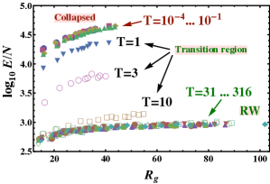
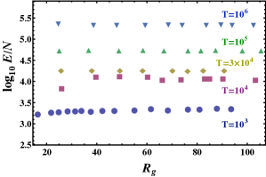
Figure 12: (Logarithm of) Specific elastic energy $E/N$ vs. the radius of gyration $R_{g}$ at different temperatures. The distinct points in the same series correspond to different numers of monomers $N$. Upper plot: the low-temperature collapsed phase and medium-temperature RW phase including the transition region between them. Lower plot: the high-temperature SARW phase. The results are fully in line with the analytic expressions (24), (27) and (29), respectively.

The lower plot of Fig. 12 describes the high-temperature SARW phase. While an increasing function of temperature, the energy now has only very weak (if any) dependence on the radius of gyration.

VI Proteins and the Huang-Lei elastic energy

In huang1 the authors propose that the elastic energy of folded proteins in PDB can be described by the following phenomenological (Huang-Lei) formula (per units of energy)

$$E_{HL}(R_{g},N)=a\,N^{4/5}+b\,(N\,R_{g})^{1/2}+c\,\frac{N^{2}}{R_{g}^{3}},$$ (32)

Here $a$, $b$ and $c$ are fitting parameters. By minimizing the energy, the authors huang1 compute for the compactness index the value

$$\nu_{HL}=3/7$$ (33)

A priori this suggests huang1 that folded proteins could be in a universality class which is different from the known ones (3).

In this Section we shall analyze the formula (32) in the context of our model. We find that it gives an accurate description of data in our model, in particular around the transition point between the collapsed phase and the RW phase where the compactness index grows continuously and monotonically from around $\nu\approx 1/3$ to around $\nu\approx 1/2$ over a finite temperature interval, due to finite scaling effects that are characteristic to a finite length chain: The value (33) corresponds to temperature value

$$T_{HL}\ \approx\ 12.5\pm 1.7$$

in our model, which suggests that we are (slightly) above the transition temperature $T_{c1}$ between collapsed and RW phases.

In figure 13 we show examples where we have fitted (32) to elastic energy computed from our model for three different values of the temperature: Deep in the collapsed phase and in the vicinity of the critical temperature $T_{c1}$ that separates the collapsed phase from the RW phase in our model. The width of the best-fit lines describes the uncertainty in the best-fit parameters, reflecting the statistical errors in our data.

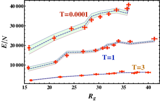
Figure 13: Three examples of the fits of the elastic energy $E$ by the Huang-Lei formula (32). The $T=0.0001$ line is deep in the collapsed phase while the $T=1$ and $T=3$ lines are both in the transition region from collapsed to RW phase, in the vicinity of the critical value $T_{c1}\approx 3.38$ .

We have found that deep in the collapsed phase the fit is not very good and consequently (32) does not describe fully collapsed proteins, as expected from the value of the compactness index. But when we enter the transition region between collapsed phase and RW phase and the compactness index starts increasing (continuously as a function of temperature for finite length chains), the quality of the fit becomes increasingly improved and in the vicinity of the critical temperature $T_{c1}$ we find for the statistical $\chi$-square parameter per degree of freedom $(dof)$ a value around

$$\chi^{2}/(dof)\approx 1$$

In figure 14 we summarize our findings for the set of best fit parameters for (32). The red-colored zones correspond to those values of temperature where the $\chi^{2}/(dof)$ parameter is very large, typically taking values around 10 and higher. In the un-colored (white) zones the $\chi^{2}/(dof)$ parameter has values that are in the vicinity of unity.

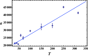
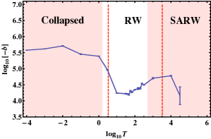
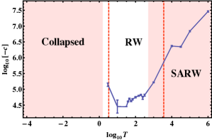
Figure 14: The best fit parameters of the fits of the elastic energy (32) are shown the log-log scale. The description is given in the text.

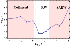
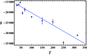
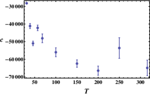
Figure 15: The parameters of the fit (32) in the RW region. The dashed lines give are the best fits given by Eqs. (35), (36), and (37).

In figure 15 we show the behavior of the parameters $a$, $b$ and $c$ in the region where the $\chi^{2}/(dof)$ values are in the vicinity of unity that is near the transition between collapsed phase and RW phase, and within the RW phase. We have found that the temperature dependence of the parameters $a$ and $b$ can be fitted by linear functions:

$$a(T)=C_{a}+\Biggl{(}1+\frac{T}{T_{a}}\Biggr{)}\$$ (34)

$$b(T)=C_{b}+\Biggl{(}1+\frac{T}{T_{b}}\Biggr{)}$$ (35)

where

$$C_{a}=8.6(1.4)\cdot 10^{3}\,,\quad\ \ \ T_{c}=216(37)\,,$$ (36)

$$C_{b}=-1.4(1)\cdot 10^{4}\,,\qquad T_{b}=246(44)\,.$$ (37)

These fits are shown in Fig. 15 by the dashed lines.

Our conclusion is that the Huang-Lei formula (32) gives a very good description of the elastic energy in our model, in particular when we are very near the transition point between the collapsed and RW phases, and slightly inside the RW phase. But it is not very accurate for temperature values that are deep in the collapsed phase, nor when we approach the cross-over to the SARW phase. We note that this is consistent with the behavior of the compactness index in our model as displayed in Fig. 2. When we compare the computed value (33) with Fig. 2 we find that this value corresponds to the transition region .

Together with huang1 , and the comparison between (15) and (16), and (14) and (21), these results suggest that our model should describe the statistical properties of folded proteins in PDB, for temperature values that are very close to the critical value $T_{c1}\approx 3.38$.

VII discussion

We have investigated the statistical properties of a homopolymer model that has been introduced to describe the properties of collapsed proteins in Protein Data Bank. We have found that as a function of temperature the model does indeed realize the three known phases of polymers: the collapsed phase, the random walk phase (RW), and the self-avoiding random walk phase (SARW). Furthermore, we have found that the model predicts that the transition between the collapsed phase and the random walk phase is a phase transition, while the random walk and self-avoiding random walk phases are separated from each other by a smooth cross-over transition. These findings are in line with general arguments on the phase structure of polymers degennes1 .

We have also computed the elastic energy as a function of radius of gyration i.e. end-to-end distance of a polymer. In the collapsed phase we have found that the energy grows faster than in Hooke’s law, in the RW phase we find Hooke’s law with temperature dependent corrections, and finally in the SARW phase we find that the dependency of energy on the radius of gyrations is weaker than in Hooke’s law. It would be interesting to test our predictions experimentally in the case of proteins, for example using atomic force microscopy.

Finally, we have compared our model with a phenomenological expression that has been introduced by Huang and Lei to describe the elastic energy of collapsed proteins. We have found that the Huang-Lei formula gives a good effective description of our model, in particular when we are in the vicinity of the transition region that separates the collapsed phase from the random walk phase. This is also consistent with our evaluation of the temperature dependence of the compactness index. When compared with the PDB data this suggests that statistical properties of collapsed proteins are indeed described by the present model in the vicinity of this transition point.

- (1) K.G. Wilson, Phys. Rev. B4 3174 (1971), ibid B4 3184 (1971)
- (2) L.P. Kadanoff, in Phase Transitions and Critical Phenomena, C. Domb and M.S. Green Eds. (Academic Press, London, 2976) Vol 5A, pp. 1-34
- (3) P.G. De Gennes, Scaling Concepts in Polymer Physics (Cornell University Press, Ithaca, 1979)
- (4) B.G. Nickel, Macromolecules 24 1358 (1991)
- (5) F.J. Wegner, Phys. Rev. B5 4529 (1972)
- (6) B. Li, N. Madras and A. Sokal, Journal of Statistical Physics 80 (1995) 661
- (7) J.C. LeGuillou and J. Zinn-Justin, Phys. Rev. B21 3976 (1980)
- (8) P.G. De Gennes, Physics Letters 38A 339 (1972)
- (9) U.H. Danielsson, M. Lundgren and A.J. Niemi, Phys. Rev. E (accepted)
- (10) K.A. Dill, O.S. Banu, M.S. Shell and T.R. Weikl, Annu. Rev. Biophys. 37 289 (2008)
- (11) Berman, H.M., Henrick, K., Nakamura, H. and Markley, J.L., Nucleic Acids Research 35 (Database issue) D301 (2007)
- (12) M. Chernodub, S. Hu and A.J. Niemi, Phys. Rev. E (accepted)
- (13) S.Hu, N. Molkenthin and A.J. Niemi (to appear)
- (14) Jinzhi Lei, and Kerson Huang, e-print arXiv:1002.5013 [cond-mat.stat-mech], e-print arXiv:1002.5024 [cond-mat.stat-mech]
- (15) C.J. Thompson, Journ. Math. Phys. 9 232 (1968)
- (16) F. Calogero, Lett. Nuovo Cimento 13 411 (1975)
- (17) M. Barma and M.E. Fischer, Phys. Rev. B31 5954 (1985)
- (18) Baker, G.A., Phys. Rev. Lett. 60 1844-1847 (1988)
- (19) The error in the estimate is large because around this point the temperature changes rapidly, indicating that we are near a phase transition.