Functional renormalization group approach to interacting bosons at zero temperature

Abstract

We investigate the single-particle spectral density of interacting bosons within the non-perturbative functional renormalization group technique. The flow equations for a Bose gas are derived in a scheme which treats the two-particle density-density correlations exactly but neglects irreducible correlations among three and more particles. These flow equations are solved within a truncation which allows to extract the complete frequency and momentum structure of the normal and anomalous self-energies. Both the asymptotic small momentum regime, where perturbation regime fails, as well as the perturbative regime at larger momenta are well described within a single unified approach. The self-energies do not exhibit any infrared divergences, satisfy the $U(1)$ symmetry constraints, and are in accordance with the Nepomnyashchy relation which states that the anomalous self-energy vanishes at zero momentum and zero frequency. From the self-energies we extract the single-particle spectral density of the two-dimensional Bose gas. The dispersion is found to be of the Bogoliubov form and shows the crossover from linear Goldstone modes to the quadratic behavior of quasi-free bosons. The damping of the quasiparticles is found to be in accordance with the standard Beliaev damping. We furthermore recover the exact asymptotic limit of the propagators derived by Gavoret and Nozières and discuss the nature of the non-analyticities of the self-energies in the very small momentum regime.

I Introduction

Interacting Bose gases in the continuum have been studied with various approaches for more than half a century, yet a controlled approach exists only for the weakly interacting variety and even there the asymptotic regime at small frequencies and momenta proved to be non-perturbative. The first qualitatively correct description of the excitation spectrum of weakly interacting bosons was given by Bogoliubov Bogoliubov1947 using a mean-field approximation. The Bogoliubov excitation spectrum exhibits the gapless linear Goldstone mode character at small wave vectors and approaches the quadratic dispersion of free bosons as wave vectors become large and interaction effects become negligible. The crossover scale separating these two regimes is given by $k_{c}=2mc$ where $m$ is the mass of the bosons and $c$ the velocity of the Goldstone modes. In dimension $D=3$, this picture has recently been confirmed experimentally using the Bragg spectroscopy technique on cold atoms.Steinhauer2002

Beliaev Beliaev58 went beyond the Bogoliubov approximation and calculated the self-energies of the quasiparticles to second order in the effective interaction, allowing both to extract corrections to the quasiparticle dispersion as well as to calculate their lifetime. However, as discussed in detail in Ref. [Shi1997, ], perturbative approaches suffer from infrared (IR) divergences for all $D\leq 3$ which are difficult to control at second order (in most physical quantities the divergences cancel out) and essentially impossible to control at any higher order of perturbation theory. These divergences have their origin in the $U(1)$ symmetry of the model and can be traced to the divergence of the longitudinal correlation function.Nepomnyashchy1975 ; Pistolesi2004 ; Vaks68 ; Patashinskii73 ; Zwerger04 Nepomnyashchy and Nepomnyashchy Nepomnyashchy1975 showed rigorously that the IR divergences, together with Ward identities originating from the $U(1)$ symmetry of the model, lead to the surprising result that the anomalous self-energy $\Sigma^{A}({\bm{k}},\omega)$ vanishes at zero momentum and frequency. This result cannot be reproduced by finite order perturbation theory, and is in sharp contrast with both the Bogoliubov and the Beliaev approach where the anomalous self-energy at zero momentum and zero frequency is finite. Furthermore, in the perturbative approaches a finite value of $\Sigma^{A}(0)$ is a key quantity which controls both the crossover to the Goldstone regime as well as the velocity of the Goldstone modes. Nepomnyashchy and Nepomnyashchy showed further that the correct structure of the self-energies contains non-analytic terms which are dominant in the asymptotic limit of small frequencies and momenta. This non-perturbative structure arises for modes with momenta smaller than the generalized Ginzburg scale $k_{G}$, which, for weakly interacting bosons, is much smaller than $k_{c}=2mc$. A correct analysis of these non-analytic terms allows to recover the Goldstone modes within a framework where $\Sigma^{A}(0)=0$. There are a number of approaches which avoid the IR divergences, the earliest is due to Popov who separated the low energy modes from the high energy modes and treated the low energy sector within a hydrodynamic theory for the phase degrees of freedom, which is free of IR divergences.Popov79 Another approach is to artificially break the $U(1)$ symmetry by a small symmetry breaking term which can in the end be removed to yield finite results for all physical observables.Capogrosso2010 A natural framework to deal with IR divergences is the renormalization group (RG). A field theoretical RG analysis of the interacting Bose gas at asymptotically small frequencies and momenta has been developed in Ref. [Pistolesi2004, ], which recovers the asymptotic behavior of the self-energies and the single particle Green’s functions. This required however a very careful analysis of Ward identities.

In several recent publications the non-perturbative or functional renormalization group (FRG) has been applied to the interacting Bose gas. Dupuis2007 ; Wetterich2007 ; SHK2009 ; Dupuis2009 ; Dupuis2009b ; Eichler09 The FRG is based on an exact flow equation of the generating functional of irreducible vertex functions (average effective action).Wetterich93 Several approaches were based on a derivative expansion of the effective action which is sufficient to find a relatively simple description of the asymptotic regime.Wetterich2007 ; Dupuis2007 One advantage of the FRG approach is that the Ward identities associated with the $U(1)$ symmetry are automatically obeyed if the truncation does not violate the invariance of the effective action. Another advantage of the FRG is that it can be employed to study the full momentum and frequency dependence of the self-energies. See Refs. [Ledowski04, ; Blaizot06, ; SHK2008, ] for FRG calculations of the momentum dependent self-energy of classical models. In Ref. [SHK2009, ] we showed how the FRG can be used to calculate the spectral density of the interacting Bose gas. This was based on a truncation of the exact FRG flow equation which respects the Nepomnyashchy relation and recovers the non-analytic structure of the low energy sector. Moreover, our FRG approach also describes the full dispersion of the Bogoliubov spectrum as well as the Beliaev damping of the quasiparticles. This is the first approach which succeeds to describe both the non-perturbative aspects which appear at the very small wavevector scale $k\ll k_{G}$, as well as the perturbative ones, which are controlled by the larger scale $k_{c}=2mc$, within a unified framework. Recently Dupuis Dupuis2009 ; Dupuis2009b developed a similar approach and clarified the role of $k_{G}$ in the flow equations, but did not resolve the Beliaev damping of the quasiparticles.

Here we present in detail our approach of Ref. [SHK2009, ] and investigate analytically the different scaling regimes of the flow equations. We further derive the flow equations for interacting Bose systems which treat the irreducible density-density interactions exactly and which has not been published previously. This set of equations, while difficult to solve, would potentially allow to analyze strongly interacting yet dilute Bose systems, which can now be realized in experiments and whose spectrum shows clear deviations from the prediction of the Beliaev approach.Papp08

This work consists of the following parts: In Sec. II we define the model and briefly review the structure of the one-particle Green’s functions, i.e. discuss the excitations and their damping. We further summarize the structure of the self-energies in the non-perturbative regime. In Sec. III we discuss the FRG approach, introduce our approximation and discuss both the general structure of the flow equations as well as the results of a derivative expansion in subsection III.1 for which we present results in $D=2$. In Sec. IV we finally discuss the results of a non-self-consistent solution of the flow equations which yields the full momentum and frequency dependence of the self-energies and allows to extract the single-particle spectral function. Numerical results are shown for $D=2$. In Appendix A we briefly review the arguments from Ref. [Nepomnyashchy1975, ] which lead to $\Sigma^{A}(0)=0$. An analysis of the derivative expansion is presented in Appendix B, where the flow of the effective interaction is analyzed analytically and the standard $T$-matrix results from diagrammatic approaches are recovered for general dimension $D$. Furthermore, in Appendix C we show how the Ginzburg scale $k_{G}$ emerges from the flow equations. In Appendix D we further show analytically, how the exact results for the asymptotic form of the normal and anomalous propagators is obtained from the non-self-consistent approach of Sec. IV. We conclude our work with a summary in Sec. V.

II Self-energies of the interacting Bose gas

We consider a system of bosons at zero temperature with a repulsive interaction potential $u_{\Lambda_{0}}(k)$. The bare microscopic action is defined in terms of the following functional of a complex field $\psi$,

$$S[\bar{\psi},\psi] = -\intop_{K}\bar{\psi}_{K}(i\omega-\epsilon_{k}+\mu)\psi_{K}$$ (1)

$$+\frac{1}{2}\intop_{K}u_{\Lambda_{0}}(k)\rho_{-K}\rho_{K},$$

where $K=(\bm{k},i\omega)$ and $\bm{k}$ is a $D$-dimensional momentum variable with the absolute value $k$ and $i\omega$ a bosonic Matsubara frequency. At zero temperature the integration over $K$ is defined as

$$\intop_{K}\equiv\intop\frac{d\omega}{2\pi}\intop\frac{d^{D}k}{(2\pi)^{D}}\,.$$ (2)

The first term of Eq. (1) describes non-interacting bosons with mass $m$ and the dispersion $\epsilon_{k}=k^{2}/2m$. The chemical potential is denoted by $\mu$. The second part represents the interaction where $\rho_{K}$ denotes the Fourier transform of the local density

$$\rho_{K}=\intop_{Q}\bar{\psi}_{Q}\psi_{Q+K}\,.$$ (3)

The subscript $\Lambda_{0}$ of $u_{\Lambda_{0}}(k)$ indicates that the theory is assumed to be regularized in the ultraviolet (UV) by a finite cutoff $\Lambda_{0}$. This cutoff is related to the finite range of the interaction; for example, for hard core interactions $\Lambda_{0}\sim 2\pi/d$, where $d$ is the diameter of the particles. The $U(1)$ symmetry of the model Eq. (1) is spontaneously broken in the ground state and the field $\psi$ acquires a finite grand canonical expectation value,

$$\phi^{0}=\big{<}\psi({\bm{r}},\tau)\big{>}\neq 0\,.$$ (4a)

A macroscopic number of particles in the ground state forms a condensate with density $\rho^{0}=|\phi^{0}|^{2}$. Because $\phi^{0}\neq 0$, the Green’s function has both normal and anomalous components. The Dyson equation for the Green’s functions in the symmetry broken state can be compactly written in a 2$\times$2 matrix in the space spanned by the field types $\psi_{K}$ and $\bar{\psi}_{K}$ as

$${\bm{G}}^{-1}(K)={\bm{G}}^{-1}_{0}(K)-{\bm{\Sigma}}(K)\,,$$ (5)

with

$${\bm{G}}(K) = \left(\begin{array}[]{cc}G^{N}(K)&G^{A}(K)\\ G^{A}(K)^{*}&G^{N}(-K)\end{array}\right)\,,$$ (8)

$${\bm{\Sigma}}(K) = \left(\begin{array}[]{cc}\Sigma^{N}(K)&\Sigma^{A}(K)\\ \Sigma^{A}(K)^{*}&\Sigma^{N}(-K)\end{array}\right)\,,$$ (11)

$${\bm{G}}_{0}^{-1}(K) = \left(\begin{array}[]{cc}G_{0}^{-1}(K)&0\\ 0&G_{0}^{-1}(-K)\end{array}\right)\,,$$ (14)

and

$$G_{0}^{-1}(K)=i\omega-\epsilon_{k}+\mu\,.$$ (15)

This leads to

$${\bm{G}}(K)=$$ (16)

$$\frac{1}{{\cal D}(K)}\left(\begin{array}[]{cc}-G^{-1}_{0}(-K)+\Sigma^{N}(-K)&\Sigma^{A}(K)\\ \Sigma^{A}(K)^{*}&-G^{-1}_{0}(K)+\Sigma^{N}(K)\end{array}\right),$$ (19)

where the denominator ${\cal D}(K)$ is given by

$${\cal D}(K) = -[G_{0}^{-1}(K)-\Sigma^{N}(K)][G_{0}^{-1}(-K)-\Sigma^{N}(-K)]$$ (20)

$$+|\Sigma^{A}(K)|^{2}.$$

We shall refer to $G^{N}(K)$ as the normal propagator and $G^{A}(K)$ as the anomalous propagator.Morawetz10 The $U(1)$ symmetry imposes constraints on the vertices among which the Hugenholtz-Pines relation for the self-energies Hugenholtz1959

$$\Sigma^{N}(0)-\Sigma^{A}(0)=\mu$$ (21)

is the best known. This equation is obeyed by the Bogoliubov approach Bogoliubov1947 which approximates both self-energies by the frequency independent leading order result $\Sigma^{N}(K)\approx\rho^{0}[u_{\Lambda_{0}}(0)+u_{\Lambda_{0}}(k)]$ and $\Sigma^{A}_{\Lambda_{0}}(K)\approx\rho^{0}u_{\Lambda_{0}}(k)$, while the condensate density is given by $\rho^{0}\approx\mu/u_{\Lambda_{0}}(0)$. This yields undamped excitations with dispersion

$$E_{k}=\sqrt{\epsilon_{k}^{2}+2\rho^{0}u_{\Lambda_{0}}(k)\epsilon_{k}}\,.$$ (22)

For small $k$ the dispersion has a Goldstone mode character with $E_{k}\sim c_{0}k$ with the velocity

$$c_{0}=\sqrt{\frac{\rho^{0}u_{\Lambda_{0}}(0)}{m}},$$ (23)

while at large momenta $E_{k}$ approaches the free particle dispersion $\epsilon_{k}=k^{2}/2m$. If $u_{\Lambda_{0}}(k)=u_{\Lambda_{0}}$ is independent of $k$, we can write

$$E_{k}=c_{0}k\sqrt{1+k^{2}/k^{2}_{0}},$$ (24)

where

$$k_{0}=2mc_{0}$$ (25)

is the mean-field estimate for the characteristic scale $k_{c}=2mc$ of the crossover from Goldstone modes to quasi-free bosons.

The leading (second order in the interaction) many-body corrections to the Bogoliubov approximation have been calculated by Beliaev. Beliaev58 At this level of approximation the single-particle excitations are damped. For $k\to 0$ the damping $\gamma_{k}$ has in three dimensions the form Beliaev58 ; Shi1997

$$\gamma^{(D=3)}_{k}=\frac{3k^{5}}{640\pi m\rho^{0}}\,.$$ (26)

while in two dimensions Kreisel2008 ; Chung2008

$$\gamma^{(D=2)}_{k}=\frac{\sqrt{3}c_{0}k^{3}}{32\pi\rho^{0}}\,.$$ (27)

The general result in $D$ dimensions can be written as Kreisel2008

$$\gamma^{(D)}_{k}\approx\alpha_{0}k^{2D-1},$$ (28)

where

$$\alpha_{0}=3^{\frac{D+1}{2}}K_{D-1}\frac{k^{3-D}_{0}}{32m\rho^{0}}\intop_{0}^{1}dx\,x^{D-1}(1-x)^{D-1}\,,$$ (29)

with

$$K_{D}=\frac{1}{2^{D-1}\pi^{D/2}\Gamma\left[D/2\right]}\,.$$ (30)

However, as discussed in detail in Ref. [Shi1997, ], already at second order the diagrams for the self-energy are in fact IR divergent and the divergent terms have to be separated from the non-divergent terms in order to obtain physical results. These divergences are in fact related to another problem common to all perturbative approaches, which is that they violate an exact result obtained by Nepomnyashchy and Nepomnyashchy, Nepomnyashchy1975 who showed that the momentum and frequency independent part of the anomalous self-energy vanishes for $D\leq 3$,

$$\Sigma^{A}(K=0)=0\,.$$ (31)

This result is a direct consequence of the IR divergences and a Ward identity relating the three point vertices to the two point vertices, see Appendix A. While in the Bogoliubov and Beliaev approach a finite value of $\Sigma^{A}(K=0)$ ensures the Goldstone character of the long wavelength modes, in the exact theory the Goldstone modes are recovered by a non-analytic structure of the self-energies which have at small frequencies and momenta the form Nepomnyashchy1975

$$\Sigma^{N}(K) \approx \rho^{0}u(K)+\mu+i\omega+a_{N}\epsilon_{k}+b_{N}\omega^{2}\;,\,\,\,\,\,\,\,$$ (32a)

$$\Sigma^{A}(K) \approx \rho^{0}u(K)+a_{A}\epsilon_{k}+b_{A}\omega^{2}\;,\,\,\,$$ (32b)

where $u(K)$ is a non-analytic function of $\omega$ and $k$ and the coefficients $a_{N},b_{N},a_{A},b_{A}$ depend on the interaction (note that the coefficient of the $i\omega$ term is exactly equal to unity Nepomnyashchy1975 ). Thus, while each of the self-energies is non-analytic for $D\leq 3$, their difference is analytic, so that the quantity

$$\sigma(K)=\Sigma^{N}(K)-\Sigma^{A}(K)-\mu$$ (33)

has the expansion

$$\sigma(K)\approx i\omega+(a_{N}-a_{A})\epsilon_{k}+(b_{N}-b_{A})\omega^{2}\,.$$ (34)

We will use in our FRG approach below a scheme where this structure of the self-energies appears naturally. As long as all irreducible correlations beyond density-density correlations can be neglected, $u(K)$ is in fact the fully renormalized density-density interaction which also completely determines the anomalous self-energy, i.e. $\Sigma^{A}(K)=\rho^{0}u(K)$.

III Functional renormalization group approach to the interacting Bose gas

We shall now set up the FRG equations for the interacting Bose gas. For recent reviews of the FRG method see Refs. [Morris98, ; Bagnuls01, ; Berges02, ; Delamotte07, ; Pawlowski07, ; PKbook, ; Rosten10, ]. The basic idea is simple and consists of introducing an IR cutoff $\Lambda$ to regulate the theory which is then sent to zero in infinitesimally small steps. The FRG follows the evolution of the various vertex functions as the IR cutoff $\Lambda$ is lowered and yields the true vertex functions for $\Lambda\to 0$. This will allow us to extract the excitation spectrum and the damping of quasiparticles from the renormalized self-energies within a theory which is free of IR divergences.

The IR divergences which plague the perturbative approaches Beliaev58 ; Shi1997 are removed if we regulate the theory by introducing a momentum cutoff $\Lambda$ in the free propagator,

$$G_{0,\Lambda}^{-1}(K)=i\omega-\epsilon_{k}+\mu-R_{\Lambda}(k)\,.$$ (35)

Here, $R_{\Lambda}(k)$ is a regulator function which removes the IR divergences arising from modes with $k<\Lambda$ and will be specified later. The FRG approach is based on the cutoff-dependent effective action which is defined by

$$\Gamma_{\Lambda}[\bar{\phi},\phi]={\cal L}_{\Lambda}[\bar{\phi},\phi]-\intop_{K}\bar{\phi}_{K}G^{-1}_{0,\Lambda}(K)\phi_{K}\,,$$ (36)

where ${\cal L}_{\Lambda}[\bar{\phi},\phi]$ is the cutoff-dependent Legendre transform of the generating functional of connected Green’s functions. The effective action is the generating functional of irreducible vertex functions, i.e. it generates cutoff-dependent irreducible vertices $\Gamma^{(n,m)}_{\Lambda}(K_{1}^{\prime},\ldots,K^{\prime}_{n};K_{m},\ldots,K_{1})$ which in the condensed phase are defined via the functional Taylor expansion of the corresponding generating functional in powers of the fluctuations $\delta\phi_{K}=\phi_{K}-\delta_{K,0}\phi_{\Lambda}^{0}$, Schuetz2005

$$\Gamma_{\Lambda}[\bar{\phi},\phi] = \sum_{n,m=0}^{\infty}\frac{1}{n!m!}\intop_{K_{1}^{\prime}}\cdots\intop_{K_{n}^{\prime}}\intop_{K_{m}}\cdots\intop_{K_{1}}$$ (37)

$$\times \delta_{K_{1}^{\prime}+\ldots+K_{n}^{\prime},K_{m}+\ldots+K_{1}}$$

$$\times \Gamma^{(n,m)}_{\Lambda}(K_{1}^{\prime},\ldots,K^{\prime}_{n};K_{m},\ldots,K_{1})$$

$$\times \delta\bar{\phi}_{K_{1}^{\prime}}\ldots\delta\bar{\phi}_{K_{n}^{\prime}}\delta{\phi}_{K_{m}}\ldots\delta{\phi}_{K_{1}}\,.$$

We normalize $\Gamma_{\Lambda}[\bar{\phi},\phi]$ such that, at the initial RG scale $\Lambda_{0}$, it reduces to the bare interaction minus the chemical potential term $\mu\intop_{K}\bar{\phi}_{K}\phi_{K}$.Eichler09 Note that $\phi_{\Lambda}^{0}$ now also has an explicit $\Lambda$-dependence which will be chosen such that $\Gamma_{\Lambda}^{(1,0)}$ and $\Gamma_{\Lambda}^{(0,1)}$ vanish for all $\Lambda$.Schuetz2005 For our purpose it is sufficient to approximate the effective action by the following ansatz,

$$\Gamma_{\Lambda}[\bar{\phi},\phi]\approx\intop_{K}\bar{\phi}_{K}\sigma_{\Lambda}(K)\phi_{K}+\frac{1}{2}\intop_{K}\delta\rho_{K}u_{\Lambda}(K)\delta\rho_{-K}\,,$$ (38)

where

$$\delta\rho_{K}=\intop_{Q}\bar{\phi}_{Q}\phi_{Q+K}-\delta_{K,0}\rho_{\Lambda}^{0}$$ (39)

is the Fourier-transform of the condensate density fluctuation $\rho(X)-\rho_{\Lambda}^{0}=\bar{\phi}_{X}\phi_{X}-\rho_{\Lambda}^{0}$. Here, in analogy with the definition of $K$, we use $X=({\bm{r},\tau})$, where $\bm{r}$ is a $D$-dimensional real space coordinate and $\tau$ is the imaginary time. At the initial UV cutoff scale $\Lambda=\Lambda_{0}$ Eq. (38) is exact and $u_{\Lambda_{0}}(K)$ is just the bare interaction which enters Eq. (1) whereas $\sigma_{\Lambda}$ vanishes initially,

$$\sigma_{\Lambda_{0}}(K)=0\,.$$ (40)

While the effective action (38) describes arbitrarily strong density-density interactions, processes which involve three or more particles are neglected. Thus, the ansatz is not expected to be accurate for dense systems but it can describe dilute yet strongly interacting ones. Note that the effective action is completely parameterized in terms of the scalar $\rho_{\Lambda}^{0}$ and the two cutoff-dependent scalar functions $\sigma_{\Lambda}(K)$ and $u_{\Lambda}(K)$. Eq. (38) represents a non-local potential approximation of the action and is explicitly $U(1)$ invariant for any value of $\Lambda$ even if the condensate density $\rho_{\Lambda}^{0}$ is finite. In the usual field expansion, the $U(1)$ symmetry of the model leads to Ward identities which relate higher order irreducible vertices to lower ones. In our approach the irreducible vertices are derived from an explicitly invariant effective action which guarantees that all Ward identities are automatically obeyed. The normal self-energy

$$\Sigma_{\Lambda}^{N}(K)=\Gamma_{\Lambda}^{(1,1)}(K,K)+\mu$$ (41)

and the anomalous self-energy

$$\Sigma_{\Lambda}^{A}(K)=\Gamma_{\Lambda}^{(2,0)}(-K,K)=\Gamma_{\Lambda}^{(0,2)}(K,-K)$$ (42)

have the form (here and below we shall assume, without loss of generality, a real valued condensate wave function $\phi_{\Lambda}^{0}$ for notational convenience)

$$\Sigma_{\Lambda}^{N}(K) = \mu+\sigma_{\Lambda}(K)+\rho_{\Lambda}^{0}u_{\Lambda}(K)\,,$$ (43a)

$$\Sigma_{\Lambda}^{A}(K) = \rho_{\Lambda}^{0}u_{\Lambda}(K)\,.$$ (43b)

Note that Eqs. (43a,43b) have the same structure as Eqs. (32a,32b) and we can already anticipate that $u_{\Lambda}(K)$ will become non-analytic for $\Lambda\to 0$ while $\sigma_{\Lambda}(K)$ will remain analytic. Moreover, since $\sigma_{\Lambda}(0)$ vanishes, Eqs. (43a,43b) obey the Hugenholtz-Pines relation (21) for all $\Lambda$. Note that Eq. (38) has no terms linear in the field $\delta\phi$ which for $\Lambda=\Lambda_{0}$ is achieved by fixing the initial condensate density as

$$\rho^{0}_{\Lambda_{0}}=\frac{\mu}{u_{\Lambda_{0}}},$$ (44)

where

$$u_{\Lambda_{0}}=u_{\Lambda_{0}}(0).$$ (45)

Eq. (38) also fixes the three- and four-point vertices of the theory which have the symmetrized form

$$\Gamma^{(2,1)}_{\Lambda}(K_{1}^{\prime},K_{2}^{\prime};K_{1}) = \phi^{0}_{\Lambda}[u_{\Lambda}(K_{1}^{\prime})+u_{\Lambda}(K_{2}^{\prime})],$$ (46)

$$\Gamma^{(1,2)}_{\Lambda}(K_{1}^{\prime};K_{2},K_{1}) = \phi^{0}_{\Lambda}[u_{\Lambda}(K_{1})+u_{\Lambda}(K_{2})],\hskip 19.91692pt$$ (47)

$$\Gamma^{(2,2)}_{\Lambda}(K_{1}^{\prime},K_{2}^{\prime};K_{2},K_{1}) = u_{\Lambda}(K_{1}^{\prime}-K_{1})+u_{\Lambda}(K_{2}^{\prime}-K_{1}).$$

These vertices are not independent but are fixed entirely by $\phi_{\Lambda}$ and $u_{\Lambda}(K)$ which can be extracted from the self-energies. This dependence is again a consequence of the $U(1)$ symmetry of the model.

For the FRG we also need the cutoff-dependent full propagators which can again be written in the form of a $2\times 2-$matrix in field type space Beliaev58

$${\bm{G}}_{\Lambda}(K) = \left(\begin{array}[]{cc}G^{N}_{\Lambda}(K)&G^{A}_{\Lambda}(K)\\ G^{A}_{\Lambda}(K)^{*}&G^{N}_{\Lambda}(-K)\end{array}\right)\,,$$ (51)

where

$$G^{N}_{\Lambda}(K) = \frac{-G^{-1}_{\Lambda,0}(-K)+\Sigma^{N}_{\Lambda}(-K)}{{\cal D}_{\Lambda}(K)}\,,$$ (52a)

$$G^{A}_{\Lambda}(K) = \frac{\Sigma^{A}_{\Lambda}(K)}{{\cal D}_{\Lambda}(K)}\,,$$ (52b)

and the denominator ${\cal D}_{\Lambda}(K)$ is given by the expression

$${\cal D}_{\Lambda}(K) = [i\omega+\epsilon_{k}-\mu+\Sigma^{N}_{\Lambda}(-K)]$$ (53)

$$\times[i\omega-\epsilon_{k}+\mu-\Sigma^{N}_{\Lambda}(K)]+|\Sigma^{A}_{\Lambda}(K)|^{2}\,.$$

The exact flow equations for the effective action $\Gamma_{\Lambda}[\bar{\phi},\phi]$ has the form Wetterich93 (here we do not keep track of the flow of the constant part of $\Gamma_{\Lambda}[\bar{\phi},\phi]$, i.e. the free energy PKbook )

$$\partial_{\Lambda}\Gamma_{\Lambda}[\bar{\phi},\phi]=\frac{1}{2}\mbox{Tr}\Big{\{}\partial_{\Lambda}\bm{G}_{0,\Lambda}^{-1}\big{[}\bm{\Gamma}^{(2)}_{\Lambda}-\bm{G}_{0,\Lambda}^{-1}\big{]}^{-1}\Big{\}}\,,$$ (54)

where

$${\bm{\Gamma}}^{(2)}_{\Lambda}[\bar{\phi},\phi] = \left(\begin{array}[]{lr}\displaystyle\frac{\delta^{2}\Gamma[\bar{\phi},{\phi}]}{\delta\bar{\phi}\,\delta{\phi}}&\displaystyle\frac{\delta^{2}\Gamma[\bar{\phi},{\phi}]}{\delta\bar{\phi}\,\delta\bar{\phi}}\\ \displaystyle\frac{\delta^{2}\Gamma[\bar{\phi},{\phi}]}{\delta{\phi}\,\delta{\phi}}&\displaystyle\frac{\delta^{2}\Gamma[\bar{\phi},{\phi}]}{\delta{\phi}\,\delta\bar{\phi}}\end{array}\right)\,.$$ (57)

Eq. (54), in conjunction with the field expansion (37), yields flow equations for the irreducible vertex functions, see e.g. Refs. [Schuetz2005, ; PKbook, ] for details.

To ensure that the field expansion (37) is always an expansion around the true minimum $\phi^{0}_{\Lambda}$, we require that $\Gamma_{\Lambda}^{(1,0)}$ and $\Gamma_{\Lambda}^{(0,1)}$ vanish for all $\Lambda$. Since for $\Lambda=\Lambda_{0}$ this is already achieved by the mean field Eq. (44), we will only need to enforce $\partial_{\Lambda}\Gamma_{\Lambda}^{(0,1)}=\partial_{\Lambda}\Gamma_{\Lambda}^{(1,0)}=0$. This yields the flow of the order parameter $\rho^{0}_{\Lambda}$,

$$\partial_{\Lambda}\rho^{0}_{\Lambda} = \frac{1}{u_{\Lambda}(0)}\intop_{Q}\Big{\{}{\dot{G}}_{\Lambda}^{N}(Q)\big{[}u_{\Lambda}(Q)+u_{\Lambda}(0)\big{]}$$ (58)

$$\hskip 56.9055pt+\dot{G}_{\Lambda}^{A}(Q)u_{\Lambda}(Q)\big{]}\Big{\}}\,,$$

which is shown diagrammatically in Fig. 1. The single scale propagators $\dot{G}_{\Lambda}^{N}$ and $\dot{G}_{\Lambda}^{A}$ which appear in Eq. (58) are defined via the matrix equation

$$\left(\begin{array}[]{cc}\dot{G}_{\Lambda}^{N}(K)&\dot{G}_{\Lambda}^{A}(K)\\ \dot{G}_{\Lambda}^{A}(K)^{*}&\dot{G}_{\Lambda}^{N}(-K)\end{array}\right)=-{\bm{G}}_{\Lambda}(K)[\partial_{\Lambda}{\bm{G}}_{0,\Lambda}^{-1}(K)]{\bm{G}}_{\Lambda}(K)\,,$$ (59)

where

$${\bm{G}}_{0,\Lambda}^{-1}(K) = \left(\begin{array}[]{cc}G_{0,\Lambda}^{-1}(K)&0\\ 0&G_{0,\Lambda}^{-1}(-K)\end{array}\right)\,.$$ (62)

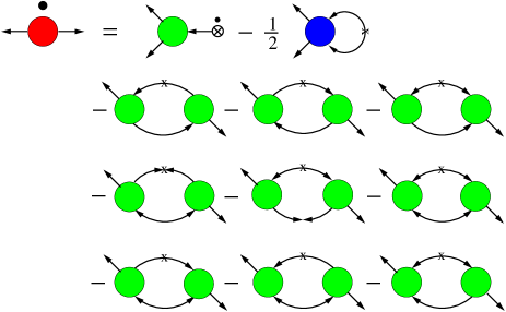
Figure 3: (Color online) Diagrammatic representation of the exact FRG flow equation for the anomalous self-energy $\Sigma_{\Lambda}^{A}(K)$. All symbols are defined as in Figs. 1 and 2.

The exact FRG flow equations for the normal and anomalous self-energies are shown diagrammatically in Figs. 2 and 3. Using the relations Eqs. (46-LABEL:eq:Gamma22trunc) for the three- and four-point vertices, the flow equations for the self-energies reduce to

$$\partial_{\Lambda}\Sigma_{\Lambda}^{N}(K) = \frac{u_{\Lambda}(K)+u_{\Lambda}(0)}{u_{\Lambda}(0)}\intop_{Q}\big{[}\dot{G}_{\Lambda}^{N}(Q)+\dot{G}_{\Lambda}^{A}(Q)\big{]}u_{\Lambda}(Q)+\intop_{Q}\dot{G}_{\Lambda}^{N}(Q)\big{[}u_{\Lambda}(K)-u_{\Lambda}(K-Q)\big{]}$$ (63a)

$$-\rho^{0}_{\Lambda}\intop_{Q}\dot{G}_{\Lambda}^{N}(Q)\Big{\{}G_{\Lambda}^{N}(K-Q)\big{[}u_{\Lambda}(Q)+u_{\Lambda}(K-Q)\big{]}^{2}+G_{\Lambda}^{N}(Q-K)\big{[}u_{\Lambda}(K)+u_{\Lambda}(K-Q)\big{]}^{2}$$

$$\hskip 22.76228pt+G_{\Lambda}^{N}(Q+K)\big{[}u_{\Lambda}(Q)+u_{\Lambda}(K)\big{]}^{2}+2G_{\Lambda}^{A}(K-Q)\big{[}u_{\Lambda}(Q)+u_{\Lambda}(K-Q)\big{]}\big{[}u_{\Lambda}(K)+u_{\Lambda}(K-Q)\big{]}\Big{\}}$$

$$-2\rho^{0}_{\Lambda}\intop_{Q}\dot{G}_{\Lambda}^{A}(Q)\Big{\{}G_{\Lambda}^{A}(K-Q)\big{[}u_{\Lambda}(K)+u_{\Lambda}(K-Q)\big{]}+G_{\Lambda}^{N}(K-Q)\big{[}u_{\Lambda}(Q)+u_{\Lambda}(K-Q)\big{]}\Big{\}}$$

$$\hskip 73.97733pt\times\,\big{[}u_{\Lambda}(K)+u_{\Lambda}(Q)\big{]}\,,$$

$$\partial_{\Lambda}\Sigma_{\Lambda}^{A}(K) = \frac{u_{\Lambda}(K)}{u_{\Lambda}(0)}\intop_{Q}\Big{\{}\dot{G}_{\Lambda}^{N}(Q)\big{[}u_{\Lambda}(Q)+u_{\Lambda}(0)\big{]}+\dot{G}_{\Lambda}^{A}(Q)u_{\Lambda}(Q)\Big{\}}-\frac{1}{2}\intop_{Q}\dot{G}_{\Lambda}^{A}(Q)\big{[}u_{\Lambda}(K+Q)+u_{\Lambda}(K-Q)\big{]}$$ (63b)

$$-\rho^{0}_{\Lambda}\intop_{Q}\dot{G}_{\Lambda}^{N}(Q)\Big{\{}\big{[}G_{\Lambda}^{N}(Q-K)+G_{\Lambda}^{N}(K-Q)\big{]}\big{[}u_{\Lambda}(K)+u_{\Lambda}(K-Q)\big{]}\big{[}u_{\Lambda}(K)+u_{\Lambda}(Q)\big{]}$$

$$\hskip 11.38092pt+\Big{(}G_{\Lambda}^{A}(K+Q)\big{[}u_{\Lambda}(Q)+u_{\Lambda}(K+Q)\big{]}+G_{\Lambda}^{A}(K+Q)\big{[}u_{\Lambda}(Q)+u_{\Lambda}(K+Q)\big{]}\Big{)}\big{[}u_{\Lambda}(Q)+u_{\Lambda}(K)\big{]}\Big{\}}$$

$$-\rho^{0}_{\Lambda}\intop_{Q}\dot{G}_{\Lambda}^{A}(Q)\Big{\{}G_{\Lambda}^{A}(K-Q)\Big{(}\big{[}u_{\Lambda}(Q)+u_{\Lambda}(K-Q)\big{]}^{2}+\big{[}u_{\Lambda}(K)+u_{\Lambda}(K-Q)\big{]}^{2}\Big{)}+G_{\Lambda}^{A}(K+Q)\big{[}u_{\Lambda}(K)+u_{\Lambda}(Q)\big{]}^{2}$$

$$\hskip 11.38092pt+\big{[}G_{\Lambda}^{N}(K-Q)+G_{\Lambda}^{N}(Q-K)\big{]}\big{[}u_{\Lambda}(K)+u_{\Lambda}(K-Q)\big{]}\big{[}u_{\Lambda}(Q)+u_{\Lambda}(K-Q)\big{]}\Big{\}}\,,$$

which, together with Eqs. (43a,43b), yield the flow equations for $\sigma_{\Lambda}(K)$ and $u_{\Lambda}(K)$. We stress that up to this point the only approximation we have made is that we only kept those irreducible correlations which are explicitly stated in the Eq. (38) for $\Gamma_{\Lambda}[\bar{\phi},\phi]$, i.e. we only consider two-body density-density correlations. However, these can be arbitrarily strong and the set of Eqs. (58,63a,63b) allow to calculate $\rho^{0}_{\Lambda}$, $u_{\Lambda}(K)$, and $\sigma_{\Lambda}(K)$, which completely determine all vertices of Eq. (38), without any further approximation. In this respect, our approach goes beyond the set of equations given in Appendix C of Ref. [Dupuis2009b, ] where additional approximations were made. While of similar complexity, the equations derived by DupuisDupuis2009b do not treat the full frequency- and momentum-dependence of the three- and four-point vertices, which appear in the flow of the self-energies, exactly. In some diagrams the dependence of these vertices on the internal frequency and momentum is neglected.

Figure 1: (Color online) Diagrammatic representation of the exact FRG flow equation for the condensate density. The circles with two external legs on the left-hand side denote the normal and anomalous self-energy. The circles with three external legs on the right-hand side denote irreducible three point vertices. Crossed circles with a dot denote the derivative of the order parameter with respect to the RG cutoff $\Lambda$, and crossed solid arrows represent normal or anomalous single scale propagators as defined in Eq. (59). Arrows pointing out of a vertex represent the fields $\bar{\psi}$, while incoming arrows represent fields $\psi$.

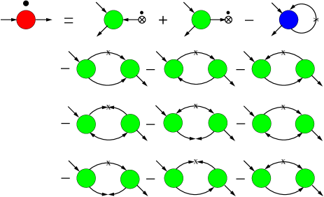
Figure 2: (Color online) Diagrammatic representation of the exact FRG flow equation for the normal self-energy $\Sigma^{N}_{\Lambda}(K)$. The circle with four external legs denotes the irreducible four-point vertex, while arrows represent cutoff-dependent normal or anomalous propagators. The dot above the two-point vertex on the left-hand side represents a derivative with respect to $\Lambda$. The other symbols are defined as in Fig. 1.

Eqs. (58,63a,63b) form a set of integro-differential equations which in principle must be solved self-consistently. While similar flow equations were recently solved exactly for a model of classical crystalline membranes,Braghin10 for the present quantum system the calculation of an exact solution is an extremely difficult problem which we will not attempt to solve. Rather, we will use a non-self-consistent approximation which is motivated by the structure of perturbation theory. Note that second order perturbation theory (including its divergences) is recovered if we replace on the right hand side of Eqs. (58,63a,63b) the full function $u_{\Lambda}(K)$ by the constant $u_{\Lambda_{0}}$ and use $\sigma_{\Lambda}=0$.

Before we calculate the full momentum and frequency dependence of the self-energies using a non-self-consistent scheme, we first consider a derivative expansion of $\Gamma_{\Lambda}$ in the next subsection.

III.1 Derivative expansion

A derivative expansion of $u_{\Lambda}(K)$ is problematic, since $u_{\Lambda}(K)$ becomes non-analytic for $\Lambda\to 0$. We therefore approximate it only by its constant part,

$$u_{\Lambda}(K)\approx u_{\Lambda}(0)=u_{\Lambda}\,.$$ (64)

This leads to a great simplification for the three- and four-point vertices. With the approximation (64) one finds from Eq. (58) the simplified form for the flow of the condensate SHK2008 ; Eichler09

$$\partial_{\Lambda}\rho^{0}_{\Lambda}=\intop_{K}\left(2\dot{G}^{N}_{\Lambda}(K)+\dot{G}^{A}_{\Lambda}(K)\right),$$ (65)

and from Eqs. (63a,63b) and (65) the simplified flows for the self-energies,SHK2009 ; Eichler09

$$\partial_{\Lambda}\Sigma^{N}_{\Lambda}(K) = 2u_{\Lambda}\intop_{Q}\left\{\dot{G}^{N}_{\Lambda}(Q)+\dot{G}_{\Lambda}^{A}({Q})\right\}-4u_{\Lambda}^{2}\rho^{0}_{\Lambda}\intop_{Q}\Big{\{}\dot{G}_{\Lambda}^{N}({Q})\big{[}G_{\Lambda}^{N}(Q+K)+G_{\Lambda}^{N}(Q-K)+G_{\Lambda}^{N}(-Q+K)$$ (66a)

$$+2G^{A}_{\Lambda}(Q-K)\big{]}+2\dot{G}_{\Lambda}^{A}(Q)\big{[}G_{\Lambda}^{A}(Q+K)+G_{\Lambda}^{N}(Q+K)\big{]}\Big{\}}\,,$$

$$\partial_{\Lambda}\Sigma^{A}_{\Lambda}(K) = 2u_{\Lambda}\intop_{Q}\dot{G}^{N}_{\Lambda}(Q)-4u_{\Lambda}^{2}\rho^{0}_{\Lambda}\intop_{Q}\Big{\{}\dot{G}^{N}_{\Lambda}(Q)\big{[}G_{\Lambda}^{N}(Q+K)+G_{\Lambda}^{N}(Q-K)+G_{\Lambda}^{A}(Q+K)+G_{\Lambda}^{A}(Q-K)\big{]}$$ (66b)

$$+\dot{G}^{A}_{\Lambda}(Q)\big{[}G_{\Lambda}^{N}(Q+K)+G_{\Lambda}^{N}(Q-K)+3G_{\Lambda}^{A}(Q+K)\big{]}\Big{\}}\,.$$

We now further employ a derivative expansion of $\sigma_{\Lambda}(K)$, which is analytic also for $\Lambda\to 0$, where we keep only the leading order terms in an expansion in $\omega$ and $k$. We thus approximate SHK2009

$$\sigma_{\Lambda}(K)\approx i\omega\left(1-Y_{\Lambda}\right)+\epsilon_{k}(Z^{-1}_{\Lambda}-1)+\omega^{2}V_{\Lambda},$$ (67)

where initially we have $Z_{\Lambda_{0}}=Y_{\Lambda_{0}}=1$ and $V_{\Lambda_{0}}=0$. With this truncation, the normal and anomalous propagators are simply

$$G^{N}_{\Lambda}(K) = \frac{Y_{\Lambda}i\omega+Z^{-1}_{\Lambda}\epsilon_{k}+\Delta_{\Lambda}+R_{\Lambda}(k)+V_{\Lambda}\omega^{2}}{{\cal D}_{\Lambda}(K)}\,,$$

$$G^{A}_{\Lambda}(K) = -\frac{\Delta_{\Lambda}}{{\cal D}_{\Lambda}(K)}\,,$$ (68b)

where

$${\cal D}_{\Lambda}(K) = Y_{\Lambda}^{2}\omega^{2}+[V_{\Lambda}\omega^{2}+Z_{\Lambda}^{-1}\epsilon_{k}+R_{\Lambda}(k)]$$ (69)

$$\times[2\Delta_{\Lambda}+V_{\Lambda}\omega^{2}+Z_{\Lambda}^{-1}\epsilon_{k}+R_{\Lambda}(k)]\,,$$

and we defined

$$\Delta_{\Lambda}=\rho_{\Lambda}^{0}u_{\Lambda}\,.$$ (70)

The corresponding single-scale propagators follow from Eq. (59). We now employ the Litim regulator Litim2001 defined through

$$R_{\Lambda}(k)=\left(1-\delta_{{k},0}\right)(2mZ_{\Lambda})^{-1}\left(\Lambda^{2}-k^{2}\right)\Theta\left(\Lambda^{2}-k^{2}\right),$$ (71)

which leads to a simplified form of the flow equations since the integration over the internal momentum can be performed trivially,

$$\intop\frac{d^{D}k}{(2\pi)^{D}}\partial_{\Lambda}R_{\Lambda}(k){\cal{F}}(k^{2})=\kappa_{\Lambda}\frac{\Lambda^{D+1}}{mZ_{\Lambda}}{\cal{F}}(\Lambda^{2}),$$ (72)

for any function ${\cal{F}}(k^{2})$. Here, we defined

$$\kappa_{\Lambda}=K_{D}[1-\eta^{z}_{\Lambda}/(D+2)]/D\,,$$ (73)

where

$$\eta^{z}_{\Lambda}=\Lambda\partial_{\Lambda}\ln Z_{\Lambda}\,$$ (74)

is the scaling dimension of $Z_{\Lambda}$ and $K_{D}$ is defined in Eq. (30). From Eqs. (65,66b) we find the flow of $\rho_{\Lambda}^{0}$ and $u_{\Lambda}$

$$\partial_{\Lambda}\rho_{\Lambda}^{0} = 4\frac{\Lambda^{D+1}\kappa_{\Lambda}}{2mZ_{\Lambda}}\int\frac{d\omega}{2\pi}\sum_{n=0}^{3}\frac{c^{(\rho)}_{n}\omega^{2n}}{{D}_{\Lambda}^{2}(i\omega)}\,,$$ (75a)

$$\partial_{\Lambda}u_{\Lambda} = 4u_{\Lambda}^{2}\frac{\Lambda^{D+1}\kappa_{\Lambda}}{2mZ_{\Lambda}}\int\frac{d\omega}{2\pi}\sum_{n=0}^{3}\frac{c^{(u)}_{n}\omega^{2n}}{{D}_{\Lambda}^{3}(i\omega)},\,\;\;$$ (75b)

where

$$D_{\Lambda}(i\omega)={\cal D}_{\Lambda}(\Lambda,i\omega)$$

$$=Y_{\Lambda}^{2}\omega^{2}+[\tilde{\epsilon}_{\Lambda}+V_{\Lambda}\omega^{2}][\tilde{\epsilon}_{\Lambda}+V_{\Lambda}\omega^{2}+2\Delta_{\Lambda}],\,\;\,$$ (76)

and we used the shorthand $\tilde{\epsilon}_{\Lambda}=\epsilon_{\Lambda}/Z_{\Lambda}$. The coefficients entering the flow (75a) are

$$c^{(\rho)}_{0} = \tilde{\epsilon}^{2}_{\Lambda}+\tilde{\epsilon}_{\Lambda}\Delta_{\Lambda}+\Delta^{2}_{\Lambda}\,,$$ (77a)

$$c^{(\rho)}_{1} = V_{\Lambda}(2\tilde{\epsilon}_{\Lambda}+\Delta_{\Lambda})-Y^{2}_{\Lambda}\,,$$ (77b)

$$c^{(\rho)}_{2} = V^{2}_{\Lambda}\,,$$ (77c)

and those entering (75b) are

$$c^{(u)}_{0} = 5\tilde{\epsilon}^{3}_{\Lambda}+3\tilde{\epsilon}^{2}_{\Lambda}\Delta_{\Lambda}+6\tilde{\epsilon}_{\Lambda}\Delta^{2}_{\Lambda}+4\Delta^{3}_{\Lambda}\,,$$ (78a)

$$c^{(u)}_{1} = 3V_{\Lambda}\left(5\tilde{\epsilon}^{2}_{\Lambda}+2\tilde{\epsilon}_{\Lambda}\Delta_{\Lambda}+2\Delta^{2}_{\Lambda}\right)$$ (78b)

$$-Y^{2}_{\Lambda}\left(7\Delta_{\Lambda}+11\tilde{\epsilon}_{\Lambda}\right)\,,$$

$$c^{(u)}_{2} = V_{\Lambda}\left[3V_{\Lambda}\left(5\tilde{\epsilon}_{\Lambda}+\Delta_{\Lambda}\right)-11Y^{2}_{\Lambda}\right]\,,$$ (78c)

$$c^{(u)}_{3} = 5V^{3}_{\Lambda}\,.$$ (78d)

To find the flow of the parameters entering $\sigma_{\Lambda}(K)$, we must expand the flow of $\Sigma^{N}_{\Lambda}(K)$, (66a), to second order in $\omega$ and $k$. This yields

$$\partial_{\Lambda}Y_{\Lambda} = -8\rho^{0}_{\Lambda}u^{2}_{\Lambda}Y_{\Lambda}\frac{\Lambda^{D+1}\kappa_{\Lambda}}{2mZ_{\Lambda}}\int\frac{d\omega}{2\pi}\sum_{n=0}^{2}\frac{c^{(y)}_{n}\omega^{2n}}{{D}_{\Lambda}^{3}(i\omega)},$$ (79a)

$$\partial_{\Lambda}Z_{\Lambda} = 4\rho^{0}_{\Lambda}u^{2}_{\Lambda}\frac{\Lambda^{D+1}K_{D}}{2mD}\int\frac{d\omega}{2\pi}\frac{1}{{D}_{\Lambda}^{2}(i\omega)}\,,$$ (79b)

$$\partial_{\Lambda}V_{\Lambda} = 8\rho^{0}_{\Lambda}u^{2}_{\Lambda}\frac{\Lambda^{D+1}\kappa_{\Lambda}}{2mZ_{\Lambda}}\int\frac{d\omega}{2\pi}\sum_{n=0}^{2}\frac{c^{(v)}_{n}\omega^{2n}}{{D}_{\Lambda}^{3}(i\omega)}\,,$$ (79c)

where the coefficients entering the flow of $Y_{\Lambda}$ are

$$c^{(y)}_{0} = \tilde{\epsilon}^{2}_{\Lambda}-2\tilde{\epsilon}_{\Lambda}\Delta_{\Lambda}-2\Delta^{2}_{\Lambda}\,,$$ (80a)

$$c^{(y)}_{1} = Y^{2}_{\Lambda}+2(\tilde{\epsilon}_{\Lambda}-\Delta_{\Lambda})V_{\Lambda}\,,$$ (80b)

$$c^{(y)}_{2} = V^{2}_{\Lambda}\,,$$ (80c)

and the coefficients entering the flow of $V_{\Lambda}$ are

$$c^{(v)}_{0} = -Y^{2}_{\Lambda}(\tilde{\epsilon}_{\Lambda}+\Delta_{\Lambda})-\tilde{\epsilon}_{\Lambda}(\tilde{\epsilon}_{\Lambda}+2\Delta_{\Lambda})V_{\Lambda}\,,$$ (81a)

$$c^{(v)}_{1} = 2V_{\Lambda}[Y^{2}_{\Lambda}+V_{\Lambda}(\tilde{\epsilon}_{\Lambda}+\Delta_{\Lambda})]\,,$$ (81b)

$$c^{(v)}_{2} = 3V^{3}_{\Lambda}\,.$$ (81c)

Before we analyze the results of the derivative expansion, let us briefly consider the scaling dimensions of the coupling parameters entering the theory. If we define the momentum to have scale one, $\left[k\right]=1$, and the dimension of frequency to be equal to the cutoff dependent dynamical exponent $\left[\omega\right]=z_{\Lambda}$, we find

$$\left[V_{\Lambda}\right] = 2-2z_{\Lambda}-\eta_{\Lambda}^{z}\,,$$ (82a)

$$\left[u_{\Lambda}\right] = 4-D-z_{\Lambda}-2\eta_{\Lambda}^{z}\,,$$ (82b)

$$\left[\rho_{\Lambda}^{0}\right] = D-2+z_{\Lambda}+\eta_{\Lambda}^{z}\,,$$ (82c)

where the scaling dimensions of $Z_{\Lambda}$ and $V_{\Lambda}$ are defined by

$$\left[Z_{\Lambda}\right] = \eta_{\Lambda}^{z}=\Lambda\partial_{\Lambda}Z_{\Lambda}\,,$$ (83a)

$$\left[Y_{\Lambda}\right] = \eta_{\Lambda}^{y}=\Lambda\partial_{\Lambda}Y_{\Lambda}\,,$$ (83b)

which fixes the dynamical exponent,

$$z_{\Lambda}=2-\eta_{\Lambda}^{z}-\eta_{\Lambda}^{y}\,.$$ (84)

Initially, we have $\eta_{\Lambda_{0}}^{z}=\eta_{\Lambda_{0}}^{y}=0$ and $z_{\Lambda_{0}}=2$ which is the correct dynamical exponent for non-interacting bosons. It is then useful to give the bare interaction strength $u_{\Lambda_{0}}$ and the chemical potential in dimensionless form,

$$\tilde{u}_{0} = 2mu_{\Lambda_{0}}\Lambda_{0}^{D-2}\,,$$ (85a)

$$\tilde{\mu} = 2m\mu_{\Lambda_{0}}\Lambda_{0}^{-2}\,.$$ (85b)

Note that at $T=0$, the scaling dimension $\eta_{\Lambda}^{z}$ plays no important role since it vanishes at $\Lambda=0$. However, at the finite temperature transition of the Bose gas the critical fluctuations lead to a finite $\eta^{z}=\lim_{\Lambda\to 0}\eta_{\Lambda}^{z}$. This was analyzed in Ref. [Eichler09, ] where the anomalous dimension $\eta^{z}$ was evaluated at the critical point. The relevant scaling dimension at $T=0$ is however $\eta^{y}_{\Lambda}$ which controls also the crossover from the $z_{\Lambda}=2$ regime to the $z_{\Lambda}=1$ regime which is characteristic of the Goldstone modes.Dupuis2007 ; Wetterich2007

Equations similar to Eqs. (75a, 75b, 79a-79c) were already discussed in Refs. [Dupuis2007, ; Wetterich2007, ; Dupuis2009, ; Dupuis2009b, ; SHK2009, ; Eichler09, ] and we briefly summarize the results for $2\leq D\leq 3$. At $T=0$ the condensate density $\rho^{0}_{\Lambda}$ flows to some finite limit $\rho^{0}_{\Lambda\to 0}=\rho^{0}>0$, while the coupling constant $u_{\Lambda}$ vanishes for $\Lambda\to 0$ which ensures $\Sigma^{N}_{\Lambda\to 0}(K=0)=\mu$ and $\Sigma^{A}_{\Lambda\to 0}(K=0)=0$, in accordance with both the Hugenholtz-Pines relation Hugenholtz1959 and the Nepomnyashchy identity.Nepomnyashchy1975 Furthermore, $Y_{\Lambda}$ vanishes for $\Lambda\to 0$, again in accordance with exact results.Nepomnyashchy1975 Since $V_{\Lambda}$ and $Z_{\Lambda}$ are finite for $\Lambda\to 0$, the low energy modes are phonons with a linear dispersion and velocity Wetterich2007 ; Dupuis2007 ; Dupuis2009 ; Dupuis2009b ; SHK2009

$$c=\frac{1}{\displaystyle\sqrt{2mVZ}}\,,$$ (86)

with $V=V_{\Lambda\to 0}$ and $Z=Z_{\Lambda\to 0}$. In Fig. 4 and Fig. 5 we show for $D=2$ the flows for the coupling parameters and for the dynamical exponent $z_{\Lambda}=2-\eta^{y}_{\Lambda}-\eta^{z}_{\Lambda}$ which illustrates the crossover from the free particle regime with $z_{\Lambda}=2$ to the Goldstone regime, where $z_{\Lambda}=1$. As pointed out by Dupuis in Refs. [Dupuis2009, ; Dupuis2009b, ], the crossover of $z_{\Lambda}$ is governed by the generalized Ginzburg scale $k_{G}$, which is indicated in Fig. 4 and Fig. 5 and is extracted from the flow equations in Appendix C. Also indicated is the crossover scale $k_{c}=2mc$. Evidently, $k_{G}$ is the relevant scale controlling the flow of the dynamical exponent $z_{\Lambda}$.Dupuis2009 ; Dupuis2009b On the other hand, the scale which determines the crossover from a linear to a quadratic behavior in the full quasiparticle dispersion is not $k_{G}$ but the crossover scale $k_{c}$, as is expected from standard perturbative approaches and as we will show in the next section when we calculate the full frequency and momentum dependence of the self-energies. It is perhaps surprising that the crossover in the momentum dependence of the quasiparticle dispersion happens at a completely different scale as the crossover in the $\Lambda$-dependence of the parameters entering the derivative expansion. In the weak-coupling regime this is however easily understood, since a quasiparticle with momentum $k$ in the range $k_{G}\ll k\ll k_{c}$ feels the largely unrenormalized bare value $u_{\Lambda_{0}}$ of the interaction potential which is sufficient to render its dispersion linear, whereas the flow of the parameters entering the derivative expansion are sensitive only to the non-perturbative effects associated with the emergence of non-analyticity at scales of the order of the Ginzburg scale $k_{G}$.

The lowest order derivative expansion is thus incapable of describing the quasiparticle dispersion beyond the asymptotic limit. Strictly speaking, even this limit is not correctly reproduced since the derivative expansion yields the unphysical result $\lim_{\Lambda\to 0}\Sigma_{\Lambda}^{A}(K)\approx\lim_{\Lambda\to 0}\rho^{0}_{\Lambda}u_{\Lambda}=0$ for all $K$, and as a consequence $\lim_{\Lambda\to 0}G_{\Lambda}^{A}(K)\to 0$. This violates an exact result by Gavoret and Nozières Gavoret1964 which is given in Eq. (90). Nonetheless, it is possible to extract the correct asymptotic form of the propagators if one cuts off the flow at a finite $\Lambda$ and uses $\Lambda\approx\sqrt{\omega^{2}+c^{2}k^{2}}$, see Refs. [Dupuis2007, ; Dupuis2009, ; Dupuis2009b, ].

Figure 4: Typical RG flows of the interaction parameter $u_{\Lambda}$ and the condensate density $\rho^{0}_{\Lambda}$ for $D=2$. The initial values are $\tilde{\mu}_{0}=2m\mu\Lambda^{-2}_{0}=0.4$ and $\tilde{u}_{0}=2mu_{\Lambda_{0}}\Lambda_{0}^{D-2}=4$. The Ginzburg scale $k_{G}$ and the crossover scale $k_{c}=2mc$ are indicated by vertical lines.

Figure 5: Typical RG flows of the coupling parameters $Y_{\Lambda}$, $Z_{\Lambda}$, $V_{\Lambda}$ and the dynamical exponent $z_{\Lambda}$ and both anomalous dimensions $\eta^{z}_{\Lambda}$ and $\eta^{y}_{\Lambda}$ in $D=2$. The initial values are the same as in Fig. 4.

IV Excitation energy and damping of quasiparticles

We now turn to the calculation of the complete frequency and momentum dependence of the self-energies from the FRG equations. As pointed out in Sec. III, a completely self-consistent solution of the flow equations (58, 63a, 63b) is numerically extremely difficult and we therefore use an approximation in which we treat only the coupling parameters of the derivative expansion of Sec. III.1 self-consistently, while all higher powers of frequency and momentum are determined in a non-self-consistent manner. A similar truncation has previously been tested for the symmetry-broken phase of a $\phi^{4}$ theory.SHK2008 A non-self-consistent solution can be quite simply achieved, starting from the approximate flow equations given in Eqs. (66a, 66b). On the right hand side of these equations we use the approximate form of the propagators given in Eqs. (68, 68b) which are based on the derivative expansion, see Eq. (64) and Eq. (67). The same approximation is employed for the single scale propagators. Note that Eqs. (68, 68b) have a sensible large $K$ behavior which for any finite $\Lambda$ and all $k>\Lambda$ are similar to the standard first order result of the Bogoliubov approximation but with a renormalized interaction parameter $u_{\Lambda}$, a renormalized condensate density $\rho^{0}_{\Lambda}$, a mass renormalization expressed by $Z_{\Lambda}$ and further a renormalized frequency dependence as expressed through $Y_{\Lambda}$ and $V_{\Lambda}$.

Using again the Litim regulator (71), the flows of the coupling parameters $u_{\Lambda}$, $\rho_{\Lambda}$, $V_{\Lambda}$, $Z_{\Lambda}$ and $Y_{\Lambda}$ can be simply obtained from the solutions of Eqs. (75a, 75b, 79a-79c). With these approximations, all parameters entering the right hand side of Eqs. (66a, 66b) are completely determined. For any $K$, we can thus simply perform the integration over $\Lambda$. With appropriate boundary conditions this yields both $\Sigma^{N}(K)$ and $\Sigma^{A}(K)$. Because of the structural similarity of both the diagrams and the propagators in this approximation to the Beliaev theory, we expect to reproduce qualitatively Beliaev’s perturbative results for both the spectrum and the damping, bar their divergences. However, since already the derivative expansion contains the key information about the non-analytic structure of the self-energies, our approach also captures these, as discussed in more detail in Appendix D.

All information about the quasiparticle properties is encoded in the single-particle spectral density which is related to the imaginary part of the real-frequency normal Green’s function,

$$A(k,\omega)=-2{\rm Im}G^{N}(k,i\omega\rightarrow\omega+i0).$$ (87)

Its calculation requires an analytical continuation to real frequencies. Here we apply the standard Padé approximant technique Vidberg which has the advantage that it can be easily implemented numerically. Although it has been originally proposed for dealing with systems at finite temperatures, it can also be used for zero-temperature calculation if the input functions are sufficiently well resolved. If it does converge, the technique is furthermore quite accurate. Applied to our problem it proved to be very robust and the results for the spectral density quickly converged for momenta which are not too small. For the actual data used to calculate the spectral density we used 450 Matsubara frequency data points for each momentum $k$. Even though the damping is quite small, this allowed to accurately extract the width of the resonance and the damping.

Figure 6: Real and imaginary parts of the normal Matsubara Green’s function as a function of $\omega$, calculated within the non-self-consistent FRG approach. The parameters are $\tilde{u}_{0}=0.8$ and $\tilde{\mu}_{0}=0.08$, which yields $k_{c}/k_{G}\approx 45$. The Green’s function is calculated for $k=0.01k_{c}\approx 0.45k_{G}$. The dashed vertical line shows the position of the minimum of the imaginary part, which coincides with the predicted resonance at $\omega=ck$.

The first task is to calculate the Matsubara normal Green’s function with satisfactory resolution. A typical result for the normal Matsubara Green’s function calculated within the non-self-consistent FRG scheme just described is shown in Fig. 6. The initial conditions for the condensate and interaction were chosen in such a way that the ratio $k_{c}/k_{G}$ remains sufficiently large (see legend below Fig. 9). We further kept the ratio $c/c_{0}$ close to unity to ensure that we are still in the weakly interacting regime. For very small momenta (we analyzed momenta down to $k=0.045k_{G}$ for $k_{c}/k_{G}\approx 45$), the real part of the normal Matsubara Green’s function indicates a resonance at $\omega=ck$; however for such small $k$ the analytic continuation no longer converged. We never found any trace of the Ginzburg scale $k_{G}$ in the properties of the normal Green’s function, which, at least in the weakly interacting regime, is perhaps expected since in the asymptotic regime the non-analytic terms are known to cancel out in the normal Green’s functions, see the discussion in Appendix D.

In order to check convergence of the Padé approach we calculated Matsubara Green’s functions for up to 450 non-equidistant frequencies in the range $0<\omega<160ck$ for each $k$ and investigated the stability of the results on increasing the number of Padé polynomials. For example, for $k_{G}\approx 0.2k_{c}$ and $k\geqslant 0.1k_{c}$ we obtain excellent convergence and a spectral density which obeys the correct normalization

$$\intop_{-\infty}^{\infty}\frac{d\omega}{2\pi}A(k,\omega)=1$$ (88)

to high accuracy. The convergence properties of the Padé approximation become continuously worse on lowering $k$ and we could not get a satisfactory analytic continuation in the non-perturbative regime $k\ll k_{G}$. However, this may be simply due to the narrowing of the peak width for small momenta. For all momenta where we do get a stable analytical continuation we find a damping which agrees qualitatively with the expected Beliaev damping, even for larger interaction strengths.

Figure 7: FRG results for the single-particle spectral density $A({k},\omega)$ as a function of the real frequency $\omega$ for different values of $k$ (top figure) and quasiparticle damping $\gamma_{k}$ (bottom figure). The shown results are for $\tilde{\mu}_{0}=0.15$ and $\tilde{u}_{0}=15$. In this case $k_{G}/k_{c}\approx 0.2$ which is indicated by the labels in the figures. The inset in the top figure shows the quasiparticle dispersion $E_{k}$ which deviates at large $k$ from linearity but is well described by a Bogoliubov type expression $E_{k}~{}=~{}\sqrt{\epsilon_{k}^{2}+c^{2}k^{2}}$ with renormalized velocity $c=(2mVZ)^{-1/2}$ (black dots). The peaks of the spectral function correspond to (from left to right) $k/k_{c}=0.2,$ $0.3,\,0.4,0.5$ and $0.6$, where $k_{c}=2mc$. In the lower plot, black dots are extracted from the spectral density, while the solid line fits them as $\gamma_{k}\approx 0.194k^{3}/2mk_{c}$.

A typical shape of the spectral density function obtained from the Padé approximation is shown in Fig. 7 for positive $\omega$. One clearly observes a finite peak broadening which can be ascribed to Beliaev damping.Beliaev58 The extracted spectrum of elementary excitations is always well fitted by a Bogoliubov-like expression $E_{k}=\sqrt{\epsilon_{k}^{2}+c^{2}k^{2}}$ and the damping of quasiparticles always reveals a $k^{3}$ behavior for $k\to 0$, in accordance with the predictions of the perturbative analysis, compare Eq. (28). However, the prefactor $\alpha_{0}$ introduced in Eq. (28) should be replaced by a function $\alpha(\tilde{\mu}_{0},\tilde{u}_{0})$ of the relevant dimensionless parameters $\tilde{\mu}_{0}$ and $\tilde{u}_{0}$ of the model (1),

$$\gamma_{k}^{(D=2)}\approx\alpha(\tilde{\mu}_{0},\tilde{u}_{0})k^{3}\,.$$ (89)

For small values of both dimensionless parameters $\tilde{\mu}_{0}$ and $\tilde{u}_{0}$ our results for the damping are very close to the perturbative result Eq. (27). For instance, for $\tilde{\mu}_{0}=0.008$ and $\tilde{u}_{0}=0.8$ we obtain $c/c_{0}\approx 1.0054$ and $\alpha(\tilde{\mu}_{0},\tilde{u}_{0})/\alpha_{0}\approx 0.967$. As both parameters increase (at fixed UV-cutoff $\Lambda_{0}$), we find a stronger renormalization of both the velocity $c$ of the Goldstone mode and of $\alpha(\tilde{\mu}_{0},\tilde{u}_{0})$. For instance, for $\tilde{\mu}_{0}=0.4$ and $\tilde{u}_{0}=4$ we obtain $c/c_{0}\approx 1.01$ and $\alpha(\tilde{\mu}_{0},\tilde{u}_{0})/\alpha_{0}\approx 0.915$, while the results for $\tilde{\mu}_{0}=0.15$ and $\tilde{u}_{0}=15$ are $c/c_{0}\approx 0.669$ and $\alpha(\tilde{\mu}_{0},\tilde{u}_{0})/\alpha_{0}\approx 0.526$. The first examples correspond to the weakly interacting regime, where many-body renormalizations are expected not to play an important role, while the last choice of the initial conditions corresponds to a more strongly interacting Bose gas where deviations from standard perturbation theory are already noticeable.

V Summary and conclusion

In conclusion, we have shown how the FRG formalism can be applied to calculate the single-particle spectral density of interacting bosons in dimensions $D\leq 3$. We here concentrated on the zero-temperature limit, but it is straightforward to extend the analysis also to finite temperatures and even to the critical temperature.Eichler09 The FRG seems to be the only presently available analytical technique which is capable of bridging the gap from the non-perturbative regime at very small frequencies and momenta, where the self-energies become non-analytic, and the intermediate to large momentum regime which is well described by the standard Beliaev theory.Beliaev58 In addition to satisfying all symmetry constraints, our approach respects the Nepomnyashchy relation for the anomalous self-energy Nepomnyashchy1975 and yields the correct asymptotic structure of the Green’s function as first derived by Gavoret and Nozières.Gavoret1964 Moreover, our approach not only reproduces the non-analytic behavior of the self-energies for scales smaller than the generalized Ginzburg scale $k_{G}$, but it also yields the standard results for the $T$-matrix renormalization in $D=2$ and $D=3$ at momentum scales larger than $k_{c}=2mc$, see Appendix B. Our approach therefore provides a single unified framework to describe the crossover from the long-wavelength Goldstone mode regime to the quasi-free boson regime where the energy dispersion is quadratic. The correct momentum dependence of the Beliaev damping, including its prefactor, can be extracted from the numerical analysis of the our truncated FRG flow equations. While we presented numerical results for the single-particle spectral density only for $D=2$, it is straightforward to apply the technique also in three dimensions.

The explicit results for the spectral function presented in this work were obtained within a non-self-consistent solution of the truncated FRG flow equations (66a,66b) for the self-energies. Although the derivative expansion has served as a guide for the derivation of Eqs. (66a,66b), our truncation scheme transcends the derivative expansion because on the right-hand side of our truncated FRG flow equations all powers of momenta and frequencies are retained. See Ref. [SHK2008, ] for a similar truncation strategy in the symmetry broken phase of classical $\phi^{4}$-theory.

Clearly, our truncation strategy will eventually fail at strong coupling. However, in principle the FRG approach, which is a non-perturbative RG technique, is well positioned also for the strong coupling regime. In fact, our truncated FRG flow equations (58,63a,63b) takes a two-body density-density interaction of arbitrary strength into account, but neglects all higher order (irreducible) correlations involving three or more particles. A solution of these flow equations, or an improved approximative solution, is nonetheless expected to give valuable insights to strongly coupled bosons.

Appendix A Elements of Nepomnyashchy theory

Gavoret and Nozières showed that both normal and anomalous propagators have the same low-energy asymptotic behavior with merely a different sign, Gavoret1964

$$G^{N}(K)\sim-G^{A}(K)\sim\frac{\rho^{0}}{\rho}\frac{mc^{2}}{\omega^{2}+c^{2}k^{2}},\;\;K\to 0,$$ (90)

where $c$ is the velocity of the Goldstone modes, $\rho^{0}$ is the condensate density and $\rho$ denotes the boson density. Note that expression (90) is an exact asymptotic result. However, as was mentioned by Gavoret and Nozières themselves, these asymptotic formulas were initially obtained by omitting divergent terms which appear in the diagrams for both self-energies. Gavoret and Nozières further assumed that $\Sigma^{A}(0)\neq 0$, which contradicts the Nepomnyashchy relation. Nepomnyashchy1975 Eq. (90) was later rederived in a formalism which is free of IR divergences and is consistent with $\Sigma^{A}(0)=0$, see Ref. [Nepomnyashchy1975, ]. We sketch here briefly the arguments which lead to the result $\Sigma^{A}(0)=0$.

The anomalous self-energy can be represented as a sum of one-particle irreducible skeleton diagrams, some of which are regular and some IR divergent,

Figure 8: Diagrams giving rise to the IR-divergent contribution (91) to the anomalous self-energy. Black dots denote the bare vertices while the shaded triangles correspond to fully renormalized vertices.

$$\Sigma^{A}(K)=\Sigma^{A}_{\rm reg}(K)+\Sigma^{A}_{\rm sing}(K),$$ (91)

where the first term on the right-hand side contains terms with a single closed Green’s function. These diagrams are regular for $K\to 0$ and $D>1$. The second term in Eq. (91) is IR divergent and arises from the diagrams shown in Fig. 8 which have the analytic form

$$\Sigma^{A}_{\rm sing}(K)=2u_{\Lambda_{0}}\sqrt{\rho^{0}}\intop_{Q}\left\{{\Gamma}^{(1,2)}(Q,K,Q-K)G^{N}(Q)G^{N}(Q-K)+{\Gamma}^{(0,3)}(Q-K;Q,-K)G^{N}(Q)G^{A}(K-Q)\right\},$$

(92)

where ${\Gamma}^{(1,2)}$ and ${\Gamma}^{(0,3)}$ are the exact irreducible vertices with two in- and one outgoing, and with three ingoing legs, respectively. The first factor $u_{\Lambda_{0}}\sqrt{\rho^{0}}$ in Eq. (92) is the value of the bare vertex ${\Gamma}_{\Lambda_{0}}^{(1,2)}$. In the limit $K=0$ and for small internal momenta $Q$ we employ the asymptotic formulas (90) and obtain

$$\Sigma^{A}(0) = \left[{\Gamma}^{(1,2)}(0,0,0)-{\Gamma}^{(0,3)}(0,0,0)\right]$$ (93)

$$\times K_{D}\intop_{0}^{\Lambda_{0}}~{}dq~{}q^{D-1}\int\frac{d\omega}{2\pi}\frac{2u_{\Lambda_{0}}\sqrt{\rho^{0}}}{(\omega^{2}+c^{2}q^{2})^{2}},\;\;$$

where the upper limit of the integration over momenta $q$ is irrelevant since we are only interested in the IR behavior of the integral. The expression in the brackets on the right-hand side of equation (93) can be further simplified by using the Ward identity Nepomnyashchy1975

$${\Gamma}^{(1,2)}(0,0,0)-{\Gamma}^{(0,3)}(0,0,0)=\frac{\Sigma^{A}(0)}{\sqrt{\rho^{0}}},$$ (94)

which, upon insertion of Eq. (94) into Eq. (93), yields an exact self-consistent equation for the anomalous self-energy. Since the integral on the right-hand side of equation (93) diverges for $D\leq 3$, the only finite solution of this equation is

$$\Sigma^{A}(0)=0.$$ (95)

Appendix B Analytic approach to the $z=2$ regime of the derivative expansion

Here we want to investigate the flow of the interaction constant $u_{\Lambda}$ in the regime where $z_{\Lambda}=2$, i.e. the initial part of the renormalization group flow. This regime yields results which are analogous to the renormalization of the $T$-matrix in both $D=2$ and $D=3$. The two-dimensional situation is especially interesting since the scattering length vanishes in $D=2$. We work out below the relevant scale which replaces the scattering length and recover the results first discussed by Schick Schick1971 who investigated the hard-core Bose gas in two dimensions using diagrammatic techniques. In $D=2$ the vanishing of $u_{\Lambda}$ for $\Lambda\to 0$ in the initial $z=2$ regime is logarithmic in $\Lambda/\Lambda_{0}$, which reflects the vanishing of the $s$-wave scattering length.Fisher1988 In the $z=2$ regime, it suffices to investigate the flow of the interaction, while setting all remaining coupling parameters of the derivative expansion to their initial values. Performing the integration over frequencies we obtain from Eq. (75b)

$$\partial_{\Lambda}u_{\Lambda} \approx u^{2}_{\Lambda}\frac{\Lambda^{D+1}K_{D}}{2mD}\frac{\epsilon^{3}_{\Lambda}-5\epsilon^{2}_{\Lambda}\Delta_{\Lambda}+\epsilon_{\Lambda}\Delta^{2}_{\Lambda}+3\Delta^{3}_{\Lambda}}{E^{5}_{\Lambda}},\;\;\;$$ (96)

where $E_{\Lambda}=\sqrt{\epsilon_{\Lambda}(\epsilon_{\Lambda}+2\Delta_{\Lambda})}$ and $\Delta_{\Lambda}=\rho_{\Lambda}^{0}u_{\Lambda}$. In the $z=2$ regime, the Bogoliubov spectrum approaches the free particle dispersion, i. e. $\epsilon_{\Lambda}\gg\Delta_{\Lambda}$. In this case we may simplify Eq. (96) as follows

$$\partial_{\Lambda}u^{-1}_{\Lambda}\approx-2m(K_{D}/D)\Lambda^{D-3}\,.$$ (97)

For $D>2$ the solution of Eq. (97) is of the form

$$u_{\Lambda}\approx\frac{u_{\Lambda_{0}}}{1+\displaystyle\frac{2mu_{\Lambda_{0}}K_{D}}{D(D-2)}\left(\Lambda^{D-2}_{0}-\Lambda^{D-2}\right)}\,.$$ (98)

For $\Lambda\to 0$ the interaction flows to a finite value which for $u_{\Lambda_{0}}\Lambda_{0}^{D-2}\gg 1$ is given by

$$u_{\Lambda\to 0}\approx\frac{u_{\Lambda_{0}}}{1+\displaystyle\frac{2mu_{\Lambda_{0}}K_{D}}{D(D-2)}\Lambda^{D-2}_{0}}\approx\frac{(D-2)a^{D-2}}{2m(2\pi)^{D-2}\kappa_{D}},$$ (99)

where we related the UV-cutoff $\Lambda_{0}\approx 2\pi/a$ to the inverse $s-$wave scattering length $a$. In $D=3$ we obtain

$$u_{\Lambda\to 0}\approx\frac{3\pi}{2m}a,$$ (100)

which is smaller than the scattering theory prediction for the $T-$matrix $8\pi a/m$ (see for instance Ref. [Shi1997, ]). However, this can be accounted for by re-adjusting the UV-cutoff to $\Lambda_{0}=3\pi/8a$. According to Eq. (98), the $s$-wave scattering length is finite in all dimensions above two.

In $D=2$, the solution of Eq. (97) has the form

$$u_{\Lambda}\approx\frac{u_{\Lambda_{0}}}{1+\displaystyle\frac{mu_{\Lambda_{0}}}{2\pi}\ln\left(\frac{\Lambda_{0}}{\Lambda}\right)}\,.$$ (101)

In the regime

$$1\gg\frac{mu_{\Lambda_{0}}}{2\pi}\ln\left(\frac{\Lambda_{0}}{\Lambda}\right)$$ (102)

the interaction does not flow and the Bogoliubov theory remains correct. The opposite case

$$1\ll\frac{mu_{\Lambda_{0}}}{2\pi}\ln\left(\frac{\Lambda_{0}}{\Lambda}\right)$$ (103)

corresponds to the limit of hard-core bosons, where the flow does not depend on the initial value of the interaction. In this case we may write

$$u_{\Lambda}\approx\frac{2\pi}{m\ln\left(\frac{\Lambda_{0}}{\Lambda}\right)},$$ (104)

which reproduces the result obtained by Fisher and Hohenberg.Fisher1988 If we now define the crossover scale where the scaling behavior of the Bogoliubov spectrum changes as $\epsilon_{\Lambda_{c}}\approx 2\rho^{0}u_{\Lambda_{c}}$, we find, setting up to logarithmic accuracy $\ln(\Lambda_{0}/\Lambda_{c})^{2}\approx 1$,

$$\Lambda^{2}_{c}\approx 16\pi\rho.$$ (105)

Hence, the corresponding energy crossover scale is given by

$$\Delta_{\Lambda_{c}}\approx\rho u_{\Lambda_{c}}\approx-\frac{8\pi\rho}{m\ln{(\rho^{0}d^{2})}},$$ (106)

which is Schick’s crossover scale for hard-core bosons,Schick1971 where $d$ is of the order of the diameter of the hard-core disc and we chose $\Lambda_{0}=\sqrt{16\pi/d^{2}}$. The velocity of the Goldstone mode in the hard-core regime becomes

$$c=\sqrt{\frac{\Delta_{\Lambda_{c}}}{2m}}\approx\sqrt{-\frac{4\pi\rho}{m^{2}\ln{(\rho d^{2})}}}\,.$$ (107)

Thus, the FRG flow equations qualitatively describe the hard-core limit.

Appendix C Asymptotic behavior of the derivative expansion

Here we derive the asymptotic $\Lambda\to 0$ behavior of the flow equations obtained within the derivative expansion, Eqs. (75a, 75b, 79a-79c), and derive from them the Ginzburg scale $k_{G}$ which is characteristic for this regime. This regime differs from the one discussed in Appendix B in that now the dynamical exponent is $z_{\Lambda}=1$. The non-perturbative character of the Bose gas is manifest in this regime.

For $\Lambda\to 0$ we may replace all coupling parameters which remain finite in this limit by their fixed point values, i.e. $Z_{\Lambda}\approx Z$, $V_{\Lambda}\approx V$, $\rho^{0}_{\Lambda}\approx\rho^{0}$. We may further approximate $\eta^{z}_{\Lambda}\approx 0$ since $\eta_{\Lambda}^{z}$ plays no important role at $T=0$. We are thus left with the flows of $u_{\Lambda}$ and $Y_{\Lambda}$. Assuming $|\omega|\leqslant c\Lambda$, where $c$ denotes the renormalized velocity of the Goldstone mode defined in Eq. (86), the small $\Lambda$ behavior of the denominator in the propagators (68) and (68b) is Dupuis2007

$$Y^{2}_{\Lambda}\omega^{2}+(\epsilon_{\Lambda}+V_{\Lambda}\omega^{2})(2\Delta_{\Lambda}+\epsilon_{\Lambda}+V_{\Lambda}\omega^{2})$$ (108)

$$\approx 2\Delta_{\Lambda}\left(\epsilon_{\Lambda}+V\omega^{2}\right)=2V\Delta_{\Lambda}(\omega^{2}+c^{2}\Lambda^{2}).$$

For small $\Lambda$, the leading contribution in the numerator of Eq. (75b) arises from the term $4\Delta^{3}_{\Lambda}$ in $c^{(u)}_{0}$ defined in Eq. (78a), since all remaining terms contain additional powers of $\epsilon_{\Lambda}\propto\Lambda^{2}$. The integration over frequencies can be carried out and the flow equation of the interaction Eq. (75b) simplifies to

$$\partial_{\Lambda}u_{\Lambda}\approx\frac{u^{2}_{\Lambda}}{A_{D}}\Lambda^{D-4},$$ (109)

where

$$A_{D}=\frac{4D}{3mk_{c}K_{D}}\left(\frac{\rho^{0}}{\rho^{s}}\right)^{2}=\frac{A^{\prime}_{D}}{mk_{c}}.$$ (110)

Here $k_{c}=2mc$ and $\rho^{s}=Z\rho^{0}$ is the superfluid density which at $T=0$ coincides with the density of bosons Dupuis2007 and

$$A^{\prime}_{D}=\frac{4D}{3K_{D}}\left(\frac{\rho^{0}}{\rho^{s}}\right)^{2}.$$ (111)

One has to distinguish between the $D<3$ and $D=3$ cases. In the first case, the general solution of Eq. (109) can be found in the form

$$u_{\Lambda}\approx\frac{u_{c}\Lambda^{\epsilon}}{\Lambda^{\epsilon}+\displaystyle\frac{mk_{c}u_{0}}{\epsilon A^{\prime}_{D}}\left[1-\left(\frac{\Lambda}{\Lambda_{c}}\right)^{\epsilon}\right]},$$ (112)

where $\epsilon=3-D$. Here, we introduced the scale $\Lambda_{c}$ and $u_{\Lambda_{c}}=u_{c}$. The scale $\Lambda_{c}$ is the characteristic scale for the boundary of the perturbative $z=2$ regime and can be approximated as $\Lambda_{c}\approx k_{c}$. At this scale, $u_{\Lambda}$ has already been renormalized by the RG flow through the perturbative $z=2$ regime, loosely defined by $\Lambda_{c}\lesssim\Lambda\lesssim\Lambda_{0}$. This in general can lead to a substantial suppression of $u_{c}$ from its bare value $u_{\Lambda_{0}}$. However, for weak coupling, for an order of magnitude estimate it is sufficient to assume $u_{c}\approx u_{\Lambda_{0}}$. In any event, the flow of the interaction for $\Lambda\ll\Lambda_{c}$ in $D<3$ neither depends on the chosen initial interaction $u_{c}$, nor on the starting value for the cutoff-parameter $\Lambda_{c}$, but only on the fully renormalized quantities entering the momentum $k_{c}$ and the factor $A^{\prime}_{D}$. For $\epsilon>0$, i. e. for $D<3$, the asymptotic expression for $u_{\Lambda}$ is in this limit given by

$$u_{\Lambda\to 0}\sim\frac{\epsilon A^{\prime}_{D}}{mk_{c}}\Lambda^{\epsilon}\,.$$ (113)

For $D<3$ the crossover from the $z=2$ to the $z=1$ regime is governed by the generalized Ginzburg scale $k_{G}$, see Refs. [SHK2008, ; Kreisel2007, ; Dupuis2009, ] which can be read off from Eq. (112)

$$k_{G}\approx\left[\frac{mk_{c}u_{0}}{\epsilon A^{\prime}_{D}}\right]^{\frac{1}{\epsilon}}\,.$$ (114)

For the weakly interacting Bose gas we have $k_{c}\approx 2mc_{0}$ and $\rho^{s}\approx\rho^{0}$. Then, $k_{G}$ may be rewritten in a form similar to the one which was obtained by Castellani et al. Pistolesi2004 and Kreisel et al., Kreisel2007

$$k_{G}\approx\left(\frac{3K_{D}}{16\epsilon D}\right)^{\frac{1}{\epsilon}}\left(\frac{k^{D}_{c}}{\rho}\right)^{\frac{1}{\epsilon}}k_{c}\,.$$ (115)

In Fig. 9 we compare of the full solution of the flow of $u_{\Lambda}$, obtained from Eqs. (75a, 75b, 79a-79c), with the approximate solution Eq. (112) for $D=2$ and different initial conditions. While solutions marked with numbers 1 and 2 in Fig. 9 correspond to a weakly interacting system (see the legend), i.e. the ratio $c/c_{0}\approx 1$, where $c$ represents the Goldstone mode velocity calculated from Eq. (86) and $c_{0}=\sqrt{\rho^{0}u_{\Lambda_{0}}/m}$ corresponds to the mean-field result for the Goldstone mode velocity, the solution marked with the number 3 corresponds to a more strongly interacting system with $c/c_{0}\approx 0.669$. It is evident that the approximate solution Eq. (112) always yields a very satisfactory approximation for $\Lambda\leqslant\Lambda_{c}$.

Figure 9: Comparison of the full numerical solution of the flow equation for the interaction $u_{\Lambda}$ as obtained from Eqs. (75a, 75b, 79a-79c) (solid lines) in $D=2$ with the approximate solution Eq. (112) (dashed lines) for different values of the bare parameters. Solutions 1 are calculated with $\tilde{u}_{0}=0.1$, $\tilde{\mu}_{0}=0.001$ which implies $k_{c}/k_{G}\approx 340$. Solutions 2 were calculated with $\tilde{u}_{0}=0.8$ and $\tilde{\mu}_{0}=0.08$ with $k_{c}/k_{G}\approx 45$. Solutions 3 are obtained with $\tilde{u}_{0}=15$ and $\tilde{\mu}_{0}=0.15$ with $k_{c}/k_{G}\approx 5$. The vertical dotted lines show positions of the Ginzburg scale for each solution.

In $D=3$, the only non-trivial solution of Eq. (109) reads

$$u_{\Lambda}\approx\frac{u_{c}}{1+\displaystyle\frac{mk_{c}u_{c}}{A^{\prime}_{3}}\ln{\displaystyle\left(\frac{\Lambda_{c}}{\Lambda}\right)}},$$ (116)

which yields the Ginzburg scale

$$k_{G}\approx\Lambda_{c}\exp\left(-\frac{A^{\prime}_{3}}{mk_{c}u_{c}}\right),$$ (117)

where $\Lambda_{c}\approx k_{c}$. In the weakly interacting regime, this expression reduces to

$$k_{G}\approx k_{c}\exp\left(-\frac{8\pi^{2}\rho^{0}}{k^{3}_{c}}\right)\,,$$ (118)

which is also consistent with the result reported in Refs. [Pistolesi2004, , Kreisel2007, ].

Analogously, from Eq. (79a) we obtain,

$$\partial_{\Lambda}Y_{\Lambda}\approx\frac{u_{\Lambda}Y_{\Lambda}}{A_{D}}\Lambda^{D-4}\,.$$ (119)

Taking in account the initial condition $Y_{c}\approx 1$, the solution of Eq. (119) reads

$$Y_{\Lambda}\approx\frac{\Lambda^{\epsilon}}{\Lambda^{\epsilon}+\displaystyle\frac{mk_{c}u_{c}}{\epsilon A^{\prime}_{D}}\left[1-\left(\frac{\Lambda}{\Lambda_{c}}\right)^{\epsilon}\right]},$$ (120)

in $D<3$, and

$$Y_{\Lambda}\approx\frac{1}{1+\displaystyle\frac{mk_{c}u_{0}}{A^{\prime}_{3}}\ln{\displaystyle\left(\frac{\Lambda_{c}}{\Lambda}\right)}}\,.$$ (121)

in $D=3$. Hence, the generalized Ginzburg scale is also characteristic for the flow of the coupling parameter $Y_{\Lambda}$.

Appendix D Asymptotic behavior of propagators in the infrared limit

We here extend the derivative expansion analysis of Sec. III.1 to include also an expansion of $u_{\Lambda}(K)$ to second order in momentum and frequency. We thus approximate

$$u_{\Lambda}(K)\approx u_{\Lambda}+\alpha_{\Lambda}\epsilon_{k}+\beta_{\Lambda}\omega^{2}\,.$$ (122)

As mentioned in Sec. III.1, the coupling function $u_{\Lambda}(K)$ is expected to become non-analytic for $\Lambda\to 0$ and this can be understood already partially from the scaling dimensions of $\alpha_{\Lambda}$ and $\beta_{\Lambda}$,

$$[\alpha_{\Lambda}] = 2-D-z_{\Lambda},$$ (123a)

$$[\beta_{\Lambda}] = 4-D-3z_{\Lambda}.$$ (123b)

In the Goldstone regime we have $z_{\Lambda}=1$ which for $D=2$ yields $[\alpha_{\Lambda}]=[\beta_{\Lambda}]=-1$, indicating that both $\alpha_{\Lambda}$ and $\beta_{\Lambda}$ diverge as $\Lambda^{-1}$ for small $\Lambda$. This suggests that for small $K$ the leading order behavior of $u_{\Lambda\to 0}(K)$ should be proportional to $k$ or $|\omega|$, which is consistent with a $\sqrt{\omega^{2}+c^{2}k^{2}}$ behavior which we find from the full frequency and momentum dependent calculation. In $D=3$, the dimensional analysis predicts $[\alpha_{\Lambda}]=[\beta_{\Lambda}]=-2$. This is suggestive of a logarithmic dependence on $|\omega|$ and $k$ which is indeed correct.

The flow equations for $\alpha_{\Lambda}$ and $\beta_{\Lambda}$ can be obtained from

$$\partial_{\Lambda}\alpha_{\Lambda} = -\frac{\alpha_{\Lambda}}{\rho^{0}_{\Lambda}}\partial_{\Lambda}\rho^{0}_{\Lambda}+\left.\frac{m}{\rho^{0}_{\Lambda}}\partial_{\Lambda}\left(\frac{\partial^{2}}{\partial k^{2}}\Sigma^{A}_{\Lambda}({\bm{k}},0)\right|_{k=0}\right),$$ (124a)

$$\partial_{\Lambda}\beta_{\Lambda} = -\frac{\beta_{\Lambda}}{\rho^{0}_{\Lambda}}\partial_{\Lambda}\rho^{0}_{\Lambda}+\left.\frac{1}{2\rho^{0}_{\Lambda}}\partial_{\Lambda}\left(\frac{\partial^{2}}{\partial\omega^{2}}\Sigma^{A}_{\Lambda}(0,\omega)\right|_{\omega=0}\right),\;\;\;\;\;\;\;\;\;$$ (124b)

where we employ a non-self-consistent approach to calculate the flows, i.e. the flows are calculated in exactly the same approximation as the full frequency and momentum dependent calculation presented in Sec. IV. The initial conditions of $\alpha_{\Lambda}$ and $\beta_{\Lambda}$ are $\alpha_{\Lambda_{0}}=0$ and $\beta_{\Lambda_{0}}=0$.

Figure 10: $\tilde{\alpha}_{\Lambda}=\Lambda^{D}_{0}\alpha_{\Lambda}$ and $\tilde{\beta}_{\Lambda}~{}=~{}2m\Lambda^{D-2}_{0}\beta_{\Lambda}$, calculated in $D=2$ for the initial values of the dimensionless chemical potential $\tilde{\mu}_{0}=2m\mu\Lambda^{-2}_{0}=0.4$ and dimensionless interaction $\tilde{u}_{0}=2mu_{\Lambda_{0}}\Lambda_{0}^{D-2}=4$.

The analytic expression for the flows is rather lengthy and can be found in Ref. [Diss, ]. The flow of the parameters $\alpha_{\Lambda}$ and $\beta_{\Lambda}$ for $D=2$ is shown in Fig. 10. The divergence of both parameters can be understood by keeping only the leading order terms of their flow equations in the limit $\Lambda\to 0$. In this case, both flow equations reduce to

$$\partial_{\Lambda}\alpha_{\Lambda}\propto\partial_{\Lambda}\beta_{\Lambda}\propto u^{2}_{\Lambda}\Lambda^{D-6}\,.$$ (125)

For $D<3$ we have from Eq. (113) $u_{\Lambda}\propto\Lambda^{3-D}$ and thus the solution of Eqs. (125) has the following small $\Lambda$ behavior,

$$\alpha_{\Lambda}\propto\beta_{\Lambda}\propto\Lambda^{1-D},$$ (126)

which agrees with the dimensional estimate for $z_{\Lambda}=1$. In $D=3$, the small $\Lambda$ behavior $u_{\Lambda}$ is proportional to $\ln(\Lambda/\Lambda_{0})$ [see Eq. (116)], so that for small $\Lambda$ Eq. (125) leads to

$$\alpha_{\Lambda}\propto\beta_{\Lambda}\propto\intop_{\Lambda}d\Lambda^{\prime}\frac{1}{(\Lambda^{\prime})^{3}\ln^{2}(\Lambda_{0}/\Lambda^{\prime})}\propto\frac{1}{\Lambda^{2}\ln(\Lambda_{0}/\Lambda)}\,\,,$$ (127)

where we have kept only the leading term. The upper integration boundary is not relevant for this estimate. Hence, using $\Lambda\sim\sqrt{\omega^{2}+c^{2}k^{2}}$, we obtain the analytical behavior of the physical anomalous self-energy in the low-energy limit in $1<D<3$,

$$\Sigma^{A}(K) \propto (\omega^{2}+c^{2}k^{2})^{\epsilon/2}\,.$$

In $D=3$, the leading behavior of the anomalous self-energy is logarithmic,

$$\Sigma^{A}(K) \propto \frac{1}{\displaystyle\ln\left(\frac{c\Lambda_{0}}{\sqrt{\omega^{2}+c^{2}{k}^{2}}}\right)}\,.$$

We are now in the position to recover the low-energy behavior of the Green’s functions. By taking Eqs. (43a, 43b, 53, 122) into account, one finds

$$G^{N}_{\Lambda}(K) = \frac{1}{{\cal D}_{\Lambda}(K)}\left[\Delta_{\Lambda}+iY_{\Lambda}\omega+(Z_{\Lambda}^{-1}+\rho^{0}_{\Lambda}\alpha_{\Lambda})\epsilon_{k}\right.$$ (128)

$$+ \left.R_{\Lambda}({k})+(V_{\Lambda}+\rho^{0}_{\Lambda}\beta_{\Lambda})\omega^{2}\right],\,\;\;\;\;$$

$$G^{A}_{\Lambda}(K) = -\frac{1}{{\cal D}_{\Lambda}(K)}\left(\Delta_{\Lambda}+\rho^{0}_{\Lambda}\alpha_{\Lambda}\epsilon_{k}+\rho^{0}_{\Lambda}\beta_{\Lambda}\omega^{2}\right),\;\;\;\;\;\;$$ (129)

$${\cal D}_{\Lambda}(K) = Y^{2}_{\Lambda}\omega^{2}+(\epsilon_{k}/Z_{\Lambda}+R_{\Lambda}({k})+V_{\Lambda}\omega^{2})$$ (130)

$$\times [(Z_{\Lambda}^{-1}+2\rho^{0}_{\Lambda}\alpha_{\Lambda})\epsilon_{k}+R_{\Lambda}({k})$$

$$+(V_{\Lambda}+2\rho^{0}_{\Lambda}\beta_{\Lambda})\omega^{2}].$$

The divergence of the parameters $\alpha_{\Lambda}$ and $\beta_{\Lambda}$ enables us to expand Eqs. (128, 129) in powers of the small quantity $\alpha^{-1}_{\Lambda}$ under the assumption $\beta_{\Lambda}/\alpha_{\Lambda}\to const$. For momenta $k\lesssim\Lambda$, we obtain to leading order of the expansion,

$$G^{N}(K) = -G^{A}(K)=\frac{1}{2V[\omega^{2}+(2mZV)^{-1}k^{2}]}$$ (131)

$$= \frac{m\rho^{0}c^{2}}{\rho}\frac{1}{\omega^{2}+c^{2}k^{2}},$$

where $\rho=\rho^{0}/Z$, and the velocity of the Goldstone mode is

$$c=\frac{1}{\sqrt{2mVZ}}\,,$$ (132)

see Eq. (86). Eq. (131) is exactly the Gavoret and Nozières resultGavoret1964 given in Eq. (90). We conclude that our non-self-consistent approach from Sec. IV both correctly describes the non-analytic behavior of the self-energies and yields the correct asymptotic behavior of the propagators. Note also that in the asymptotic result (131) the scale $k_{G}$ and all of the non-analytic behavior of the self-energies is completely absent and it remains an open problem whether and how the non-perturbative scale $k_{G}$ shows up in the spectrum or damping of quasiparticles. The scale does however emerge quite dramatically in the so-called longitudinal Green’s function which is defined and discussed e.g. in Refs. [Pistolesi2004, ; Dupuis2009, ; Dupuis2009b, ]. While for usual Bose systems the longitudinal Green’s function is not accessible to experiments, in antiferromagnetic materials, subject to strong magnetic fields close to the saturation field strength, it is possible to directly probe the spectral properties of the longitudinal Green’s function,Kreisel2007 which is related to the longitudinal spin structure factor of the underlying spin model.

References

• (1) N. N. Bogoliubov, Izv. AN SSSR Ser. Fiz. 11, 77 (1947) [J. Phys. (Moscow) 11, 23 (1947)].
• (2) J. Steinhauer, R. Ozeri, N. Katz, and N. Davidson, Phys. Rev. Lett. 88, 120407 (2002); R. Ozeri, N. Katz, J. Steinhauer, and N. Davidson, Rev. Mod. Phys. 77, 187 (2005).
• (3) S. T. Beliaev, Zh. Eksp. Teor. Fiz. 34, 417 (1958), ibid. 433 (1958) [Sov. Phys. JETP 7, 289 (1958); ibid. 7, 299 (1958)].
• (4) H. Shi and A. Griffin, Phys. Rev. 304, 1 (1998).
• (5) A. A. Nepomnyashchy and Yu. A. Nepomnyashchy, Pis’ma Zh. Eksp. Teor. Fiz. 21, 3 (1975) [JETP Lett. 21, 1 (1975)], and Zh. Eksp. Teor. Fiz. 75, 976 (1978) [Sov. Phys. JETP 48, 493 (1978)]; Yu. A. Nepomnyashchy, Zh. Eksp. Teor. Fiz. 85 1244 (1983) [Sov. Phys. JETP 58, 722 (1983)].
• (6) C. Castellani, C. Di Castro, F. Pistolesi, and G. C. Strinati, Phys. Rev. Lett. 78, 1612 (1997); F. Pistolesi, C. Castellani, C. Di Castro, and G. C. Strinati, Phys. Rev. B 69, 024513 (2004).
• (7) V. G. Vaks, A. I. Larkin, and S. A. Pikin, Zh. Eksp. Teor. Fiz. 53, 1089 (1967) [Sov. Phys. JETP 26, 188 (1968)].
• (8) A. Z. Patashinskii and V. L. Pokrovskii, Zh. Eksp. Teor. Fiz. 64, 1445 (1973) [Sov. Phys. JETP 37, 733 (1973)].
• (9) W. Zwerger, Phys. Rev. Lett. 92, 027203 (2004).
• (10) V. Popov and A. V. Seredniakov, Zh. Eksp. Teor. Fiz. 77, 377 (1979) [Sov. Phys. JETP 50, 193 (1979)].
• (11) B. Capogrosso-Sansone, S. Giorgini, S. Pilati, L. Pollet, N. Prokofev, B. Svistunov, and M. Troyer, New J. Phys. 12, 043010 (2010).
• (12) N. Dupuis and K. Sengupta, Europhys. Lett. 80, 50007 (2007).
• (13) C. Wetterich, Phys. Rev. B 77, 064504 (2008); S. Floerchinger and C. Wetterich, ibid. 77, 053603 (2008); Phys. Rev. A 79, 013601 (2009).
• (14) A. Sinner, N. Hasselmann, and P. Kopietz, Phys. Rev. Lett. 102, 120601 (2009).
• (15) N. Dupuis, Phys. Rev. Lett. 102, 190401 (2009).
• (16) N. Dupuis, Phys. Rev. A 80, 043627 (2009).
• (17) C. Eichler, N. Hasselmann, and P. Kopietz, Phys. Rev. E 80, 051129 (2009).
• (18) C. Wetterich, Phys. Lett. B 301, 90 (1993).
• (19) S. Ledowski, N. Hasselmann, and P. Kopietz, Phys. Rev. A 69, 061601(R) (2004); N. Hasselmann, S. Ledowski, and P. Kopietz, ibid. 70, 063621 (2004).
• (20) J.-P. Blaizot, R. Méndez-Galain, and N. Wschebor, Phys. Rev. E 74, 051116 (2006); ibid. 74, 051117 (2006).
• (21) A. Sinner, N. Hasselmann, and P. Kopietz, J. Phys.: Cond. Mat. 20, 075208 (2008).
• (22) S. B. Papp, J. M. Pino, R. J. Wild, S. Ronen, C. E. Wieman, D. S. Jin, and E. A. Cornell, Phys. Rev. Lett. 101, 135301 (2008).
• (23) An alternative approach, which relates the anomalous self-energy to the $T$-matrix of the channel in which the condensate appears, can be found in K. Morawetz, arXiv:0911.17525 and M. Männel, K. Morawetz, P. Lipavský, New J. Phys. 12, 033013 (2010).
• (24) N. M. Hugenholtz and D. Pines, Phys. Rev. 116, 489 (1959).
• (25) A. Kreisel, F. Sauli, N. Hasselmann, and P. Kopietz, Phys. Rev. B 78, 035127 (2008).
• (26) M. C. Chung and A. B. Bhattacherjee, New J. Phys. 11, 123012 (2009).
• (27) T. R. Morris, Prog. Theor. Phys. 131, 395 (1998).
• (28) C. Bagnuls and C. Bervillier, Phys. Rept. 348, 91 (2001).
• (29) J. Berges, N. Tetradis, and C. Wetterich, Phys. Rept. 363, 223 (2002).
• (30) B. Delamotte, cond-mat/0702365.
• (31) J. M. Pawlowski, Annals Phys. 332, 2831 (2007).
• (32) P. Kopietz, L. Bartosch, and F. Schütz, Introduction to the Functional Renormalization Group, (Springer, Berlin, 2010).
• (33) O. Rosten, arXiv:1003.1366v3 [hep-th].
• (34) F. Schütz and P. Kopietz, J. Phys. A 39, 8205 (2006).
• (35) F. L. Braghin and N. Hasselmann, Phys. Rev. B 82, 035407 (2010).
• (36) D. F. Litim, Phys. Rev. D 64, 105007 (2001).
• (37) J. Gavoret and P. Nozières, Ann. Phys. 28, 349 (1964).
• (38) H. J. Vidberg and J. W. Serene, J. Low Temp. Phys. 29, 179 (1977).
• (39) M. Schick, Phys. Rev. A 3, 1067 (1971).
• (40) D. S. Fisher and P. C. Hohenberg, Phys. Rev. B 37, 10 (1988).
• (41) A. Kreisel, N. Hasselmann, and P. Kopietz, Phys. Rev. Lett. 98, 067203 (2007).
• (42) A. Sinner, Application of the Functional Renormalization Group to Bose systems with broken symmetry, PhD thesis, Universität Frankfurt (2009); http://publikationen.ub.uni-frankfurt.de/volltexte/2009/6800/.