Museo Storico della Fisica, Centro Studi e Ricerche E. Fermi,
Piazza del Viminale 1, I-00184 Roma, Italy. Scuola Normale Superiore, Piazza dei Cavalieri 7, I-56123 Pisa, Italy. INFN, Sezione di Pisa, Largo Fibonacci 3, I-56127, Pisa, Italy. 14.65.Ha Top quarks12.38.Bx Perturbative calculations

Theoretical issues on the top mass reconstruction
at hadron colliders

Abstract

I discuss a few selected topics related to the reconstruction of the mass of the top quark at hadron colliders. In particular, the relation between the measured top mass and theoretical definitions, such as the pole or $\overline{\rm{MS}}$ mass, is debated. I will also summarize recent studies on the Monte Carlo uncertainty due to the fragmentation of bottom quarks in top decays.

The top quark is an essential ingredient of the Standard Model of the fundamental interactions and the determination of its properties provides important tests of the strong and electroweak interactions. In particular, the top quark mass ($m_{t}$) plays a crucial role in the precision tests of the Standard Model, as the combination of $m_{t}$ with the $W$-boson mass $m_{W}$ constrains the mass of the Standard Model Higgs boson (see, e.g., the updated results from the LEP electroweak working group [1]). Moreover, the top mass, along with $m_{W}$ and the mass of a possibly discovered Higgs boson, is a relevant parameter to discriminate among New Physics scenarios, such as the Minimal Supersymmetric Standard Model [2]. The latest top mass measurement at the Tevatron accelerator is $m_{t}=(173.3\pm 1.1)$ GeV [3]. However, it is often unclear how to relate the measured $m_{t}$ to a consistent mass definition.

In fact, from the theoretical point of view, several mass definitions exist, according to how one subtracts the ultraviolet divergences in the renormalized self-energy $\Sigma(p,m_{t},\mu)$, where $p$ is the momentum of the top quark, assumed to be off-shell, and $\mu$ the renormalization scale. The pole mass, often used in decay processes of on-shell particles, is thus defined by means of the conditions $\Sigma(p)=0$ and $\partial\Sigma/\partial\not p=0$ for $\not p=m_{t}$. The pole mass works well for leptons, such as electrons, whereas, when dealing with heavy quarks, it presents the so-called non-perturbative ambiguity, i.e. an uncertainty $\Delta m\sim\Lambda_{\rm{QCD}}$. In other words, after including higher-order corrections, the self-energy, expressed in terms of the pole mass $m_{t}$, exhibits in the infrared regime a renormalon-like behaviour:

$$\Sigma(m_{t})\sim m_{t}\ \sum_{n}\ \alpha_{S}^{n+1}\ (2\beta_{0})^{n}\ n!,$$ (1)

where $\beta_{0}$ is the first coefficient of the QCD $\beta$-function.

Another definition of top mass which is often used is the $\overline{\rm{MS}}$ mass, namely $\bar{m}_{t}(\mu)$, corresponding, e.g. in dimensional regularization with $D=4-2\epsilon$ dimensions, to subtracting off the renormalized self-energy the quantity $1/\epsilon+\gamma_{E}-\ln(4\pi)$, $\gamma_{E}$ being the Euler constant. The $\overline{\rm{MS}}$ mass is a suitable mass definition in processes where the top quarks are off-shell; in fact, by means of this definition, one is able to reabsorb in $\bar{m}_{t}(\mu)$ contributions $\sim\ln(\mu^{2}/m_{t}^{2})$, which are large if $\mu$ is taken of the order of the hard scale $Q$ and $Q\gg m_{t}$. For $t\bar{t}$ production at threshold, nonetheless, the $\overline{\rm{MS}}$ mass is not an adequate mass scheme, since it exhibits contributions $\sim(\alpha_{S}/v)^{k}$, $v$ being the top quark velocity, which are enhanced for $v\to 0$. Of course, one can always relate pole and $\overline{\rm{MS}}$ masses by means of a relation like [5]:

$$m_{t}=\bar{m}_{t}(\mu)\left[1+\alpha_{S}(\mu)c_{1}+\alpha_{S}^{2}(\mu)c_{2}+\dots\right],$$ (2)

where the coefficients $c_{i}$ depend on $\ln[\bar{m}_{t}^{2}(\mu)/\mu^{2}]$.

Besides pole and $\overline{\rm{MS}}$ schemes, other mass definitions for heavy quarks have been proposed. For example, in the potential-subtracted (PS) mass a counterterm $\delta m_{t}$ is constructed in such a way to remove the renormalon ambiguity in the infrared regime at the factorization scale $\mu_{F}$. It is given by [4]:

$$m_{t,\mathrm{PS}}(\mu_{F})=m_{t}-\delta m_{t}(\mu_{F}),$$ (3)

where the subtracted term reads

$$\delta m(\mu_{F})=\frac{1}{2}\int_{|q|<\mu_{F}}{\frac{d^{3}q}{(2\pi)^{3}}}\tilde{V}(q),$$ (4)

$\tilde{V}(q)$ being the Fourier transform of the $t\bar{t}$ Coulomb potential. More generally, one can define several short-distance masses in terms of a parameter, usually called $R$, corresponding, e.g., to the factorization scale $\mu_{F}$ or the $\overline{\rm{MS}}$ mass, so that the pole mass $m_{t}$ can be expressed in terms of a $R$-dependent renormalized mass and a counterterm [6]:

$$m_{t}=m_{t}(R,\mu)+\delta m_{t}(R,\mu).$$ (5)

In Eq. (5) $\delta m_{t}(R,\mu)$ can be expanded as a series of the strong coupling constant, whereas $m_{t}(R,\mu)$ satisfies a renormalization-group equation:

$$\delta m_{t}(R,\mu)=R\sum_{n=1}^{\infty}\sum_{k=0}^{n}a_{nk}\alpha_{S}^{n}(\mu)\ \ ,\ \ \frac{dm(R,\mu)}{d\ln\mu}=-R\gamma[\alpha_{S}(\mu)],$$ (6)

with $\gamma[\alpha_{S}(\mu)]$ playing the role of the anomalous dimension [6].

In order to make a statement on the top quark mass which is extracted from the data, in principle one should compare the measurement of a quantity depending on the top mass with a calculation which uses a consistent definition, e.g. the pole or the $\overline{\rm{MS}}$ mass. The D0 Collaboration [7] compared the measured total $t\bar{t}$ cross section with the calculations [8] and [9]. Ref. [8] computes the $t\bar{t}$ cross section at next-to-leading order (NLO) and resums soft/collinear contributions in the next-to-next-to-leading logarithmic (NLL) approximation. The calculation [9] is NLO, resums the Sudakov logarithms of the top velocity $\alpha_{S}^{4}\ln^{k}v$, with $k\leq 4$, and includes Coulomb contributions $\sim 1/v$ and $\sim 1/v^{2}$ to next-to-next-to-leading order (NNLO). Comparing the experimental cross section with the formulas in Refs. [8, 9], one can extract the top mass employed in such calculations. Using the pole mass, which is a reasonable assumption since top quarks are slightly above threshold at the Tevatron, one obtains the following results [7]: $m_{t}=171.5^{+9.9}_{-8.8}$ GeV, according to [8], $m_{t}=173.1^{+9.8}_{-8.6}$ GeV when using [9].

Furthermore, in Ref. [9] the computation was carried out in the $\overline{\rm{MS}}$ renormalization scheme, and $\bar{m}_{t}(\bar{m}_{t})$ was extracted from the comparison with the measured cross section. Fig. 1, taken from Refs. [7, 9] shows the main results of such a comparison.

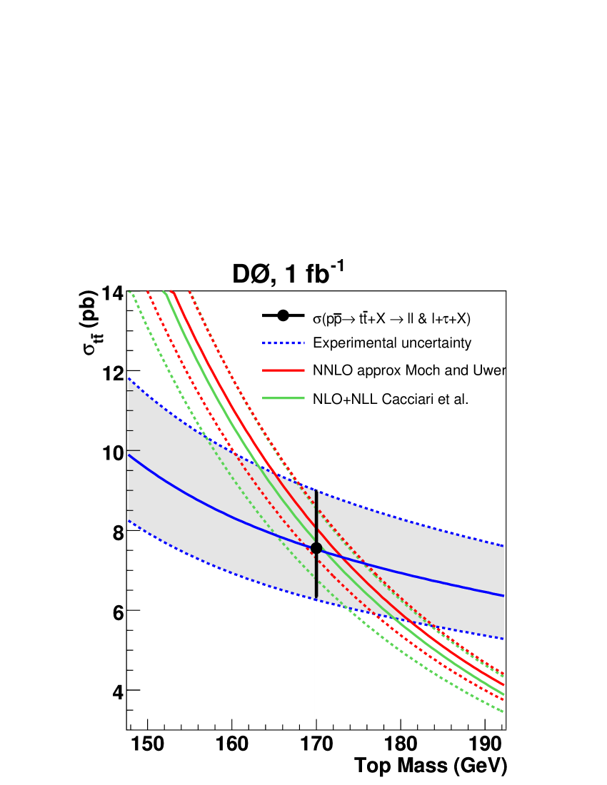
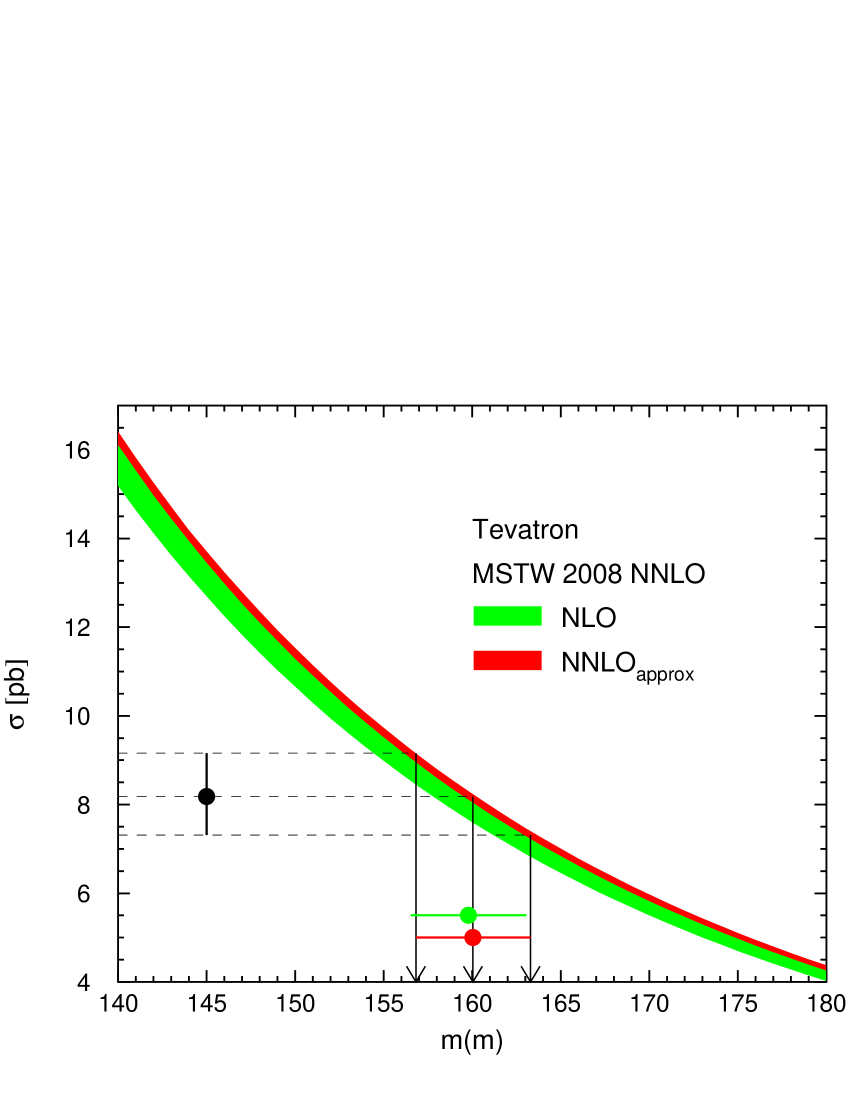
Figure 1: Left: Extraction of the top pole mass by comparing the D0 cross section with the computations [8, 9]. Right: Determination of the $\overline{\rm{MS}}$ mass following [9].

From $\bar{m}_{t}(\bar{m}_{t})$ one can determine the pole mass $m_{t}$: the central values are reported in Table 1, whereas the errors are quoted in [9].

	$\bar{m}_{t}(\bar{m}_{t})$	$m_{t}$
LO	159.2 GeV	159.2 GeV
NLO	159.8 GeV	165.8 GeV
NLO+ NNLO approx.	160.0 GeV	168.2 GeV

Table 1: Extracted values of the pole and $\overline{\rm{MS}}$ top mass comparing the computation [9] with the D0 $t\bar{t}$ cross section. See [9] for the errors on the quoted numbers.

Ref. [9] also found out that using the $\overline{\rm{MS}}$ top mass leads to a milder dependence of the cross section on factorization and renormalization scales, with respect to the pole mass. This result is indeed quite cumbersome, since, in principle, at the Tevatron top quarks are almost at threshold; the possible full inclusion of NNLO terms should probably shed light on the uncertainty when using pole or $\overline{\rm{MS}}$ masses.

Although the D0 determination of the top mass by using fixed-order and possibly resummed calculations is surely very interesting, the standard Tevatron analyses [3], such as the template or matrix-element methods, are driven by Monte Carlo parton shower generators, such as HERWIG [10] and PYTHIA [11]. Such algorithms simulate multiple radiation in the soft/collinear approximation and are possibly supplemented by matrix-element corrections to include hard and large-angle emissions. Moreover, the yielded total cross section is LO, whereas differential distributions are equivalent to leading-logarithmic soft/collinear approximation, with the inclusion of some NLLs [12]. The hadronization transition is finally implemented according to the cluster model [13] in HERWIG and the string model [14] in PYTHIA.

The template and matrix-element methods rely on the Monte Carlo description of top decays. As discussed above, when looking at top decays near threshold, the reconstructed top mass should be close to the pole mass and the world average actually agrees, within the error ranges, with the pole mass extracted from NLO cross section calculations. However, as parton shower generators are not NLO computations, there are several uncertainties which affect the correspondence between the mass which is implemented and any mass definition and renormalization scheme. Monte Carlo algorithms neglect width and interference effects, but just factorize top production and decay; this is a reasonable approximation as long as one sets cuts on the transverse energy of final-state jets much higher than the top width $\Gamma_{t}$. Nevertheless, the quoted systematic and statistical errors on the top mass [3] are competitive with the top width. Furthermore, top decays ($t\to bW$) in both HERWIG and PYTHIA are matched to the exact tree-level $t\to bWg$ calculation [15, 16], but the virtual corrections in the top-quark self-energy, which one must calculate to consistently define a renormalization scheme, are included only in the soft/collinear approximation by means of the Sudakov form factor. Also, other uncertainties are associated with the flow of the colour of the top quarks and with the hadronization corrections, since all measured observables are at hadron-level.

In principle, higher-order calculations are available even for top decays: Refs. [17, 18] calculated the $b$-quark spectrum in top decay at NLO and included NLL soft/collinear resummation in the framework of perturbative fragmentation functions. Nevertheless, such calculations are too inclusive to be directly used in the Tevatron analyses; also, the results are expressed in terms of the $b$-quark ($B$-hadron) energy fraction in top rest frame, which is a difficult observable to measure. Ref. [19] recently computed several quantities relying on top decays at NLO using the top pole mass: a comparison of this calculation with Tevatron or LHC data, though not carried out so far, should possibly provide another consistent determination of the pole mass.

An attempt to associate the Monte Carlo top mass with a formal mass definition has been carried out in [6, 20, 21, 22] in the framework of Soft Collinear Effective Theories (SCET). According to this approach, valid in the regime $Q\gg m_{t}\gg\Gamma_{t}\gg\Lambda_{\rm{QCD}}$, where $Q$ is the process hard scale, one can factorize the double-differential cross section in terms of the top ($M_{t}$) and antitop ($M_{\bar{t}}$) invariant-mass squared as follows:

$$\frac{d\sigma}{dM_{t}^{2}dM_{\bar{t}}^{2}}=\sigma_{0}H_{Q}H_{m}\int{d\ell^{+}d\ell^{-}}B_{+}\left(\ell^{+},\Gamma_{t}\right)B_{-}\left(\ell^{-},\Gamma_{t}\right)S(\ell^{+},\ell^{-}).$$ (7)

In Eq. (7), $H_{Q}$ and $H_{m}$ are hard-scattering coefficient functions at scales $Q$ and $m_{t}$, $B_{\pm}$ are the so-called heavy-quark jet functions, describing the evolution of top quarks into jets, $S(\ell^{+},\ell^{-},\mu)$ is named soft function and is a non-perturbative fragmentation function, depending on soft radiation and ruling the dijet and mass distributions. When writing a factorization formula like in (7), large logarithms of the scale ratios, such as $\ln(Q/m_{t})$ or $\ln(m_{t}/\Gamma_{t})$, clearly arise: the jet function has been resummed to NNLL in $e^{+}e^{-}$ annihilation, the soft one to NLL [20].

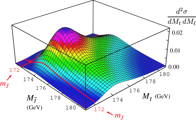
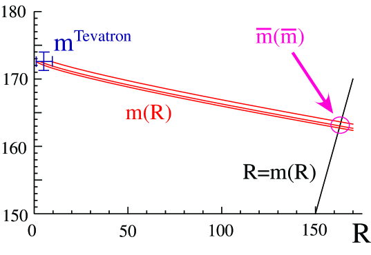
Figure 2: Left: Double differential resummed cross section with respect to the top and antitop invariant masses. Right: $R$-evolution from the Tevatron top mass, corresponding to $R\simeq 1$ GeV, to the $\overline{\rm{MS}}$ mass, i.e. $R\simeq\bar{m}_{t}(\bar{m}_{t})$.

The peak value of the distribution $d^{2}\sigma/(dM_{t}^{2}dM_{\bar{t}}^{2})$, displayed in Fig. 2 in the NLL approximation for $e^{+}e^{-}\to t\bar{t}$ processes, is independent of the mass scheme and can be expressed in terms of a short-distance mass $m$, $\Gamma_{t}$, $Q$ and $\Lambda_{\rm{QCD}}$:

$$M_{t}^{\mathrm{peak}}=m+\Gamma_{t}(c_{1}\alpha_{S}+c_{2}\alpha_{S}^{2}+\dots)+\frac{c_{3}Q\Lambda_{\rm{QCD}}}{m},$$ (8)

where the term $\sim\Gamma_{t}$ depends on the jet function and the one $\sim\Lambda_{\rm{QCD}}$ on the soft function. The jet mass is thus constructed as a short-distance mass, defined following Eq. (5), with the parameter $R\sim\Gamma_{t}$ and the counterterm $\delta m_{J}$ depending on the jet function. Expressing $M_{t}^{\mathrm{peak}}$ in terms of the pole ($m_{t}$) and jet ($m_{J}$) masses, one can finally relate $m_{t}$ and $m_{J}(\mu)$ [21]:

$$m_{t}=m_{J}(\mu)+e^{\gamma_{E}}\Gamma_{t}\frac{\alpha_{S}(\mu)C_{F}}{\pi}\left(\ln\frac{\mu}{\Gamma_{t}}+\frac{1}{2}\right)+{\cal O}(\alpha_{S}^{2}).$$ (9)

One can note that a correction $\sim\Gamma_{t}$ arises in the difference between the pole and jet masses: in fact, it was pointed out above that the top width was one of the ambiguities when associating the top mass reconstructed from final-state decay observables, e.g. the jet mass, with the pole mass. Ref. [22] then assumed that the jet mass should correspond to the mass in the event generators and measured at the Tevatron with $\mu$ being of the order of the hadronization scale (shower cutoff), i.e. $\mu\simeq Q_{0}\simeq 1$ GeV. Using the $R$-evolution equations (5), with $m_{J}(Q_{0})\simeq$ 172 GeV, one can finally obtain the $\overline{\rm{MS}}$ mass $\bar{m}_{t}(\bar{m}_{t})\simeq 163.0$ GeV [22] (see Fig. 2). Refs. [6, 21, 22] seem therefore to indicate a possible strategy to relate the mass parameter in the Monte Carlo codes to pole and $\overline{\mathrm{MS}}$ masses. However, as discussed also in [22], the situation at hadron colliders is more complicated and, before drawing a final conclusion, one would need to take into account effects, such as initial-state radiation, hadronization and underlying event, which are included in Monte Carlo event generators, but not yet in the factorization formula (7), which has been worked out for $e^{+}e^{-}$ annihilation. Further studies aiming at extending the factorization (7) to hadron colliders are certainly worth to be pursued.

In fact, the theoretical error on the top mass determination is a crucial issue, even for the sake of the Standard Model precision tests. Ref. [23] presents an analysis aimed at assessing the uncertainty due to the treatment of bottom-quark fragmentation in top decays in HERWIG and PYTHIA. For this scope, one should tune the cluster and string models to the same data sets: Ref. [24] found out that the default parametrizations are unable to reproduce LEP and SLD data on $B$-hadron production in $e^{+}e^{-}$ annihilation, but it was necessary to fit the hadronization models to obtain an acceptable description of such data. As in [23], an interesting observable is the invariant mass $m_{B\ell}$ in the dilepton channel, where $B$ is a $b$-flavoured hadron in top decay and $\ell$ a lepton from $W$ decay $W\to\ell\nu$. A reliable description of $m_{B\ell}$ is essential in the study [25] (see also Chapter 8 in Ref. [26]), wherein the top mass is reconstructed by means of the $m_{J/\psi\ell}$ spectrum, with the $J/\psi$ coming from $B\to J/\psi$ decays, and in the analysis [27], which investigates semileptonic decays $B\to\mu X$ and extracts the top mass from the $m_{\mu\ell}$ distribution. Moreover, the $B$-lepton invariant mass was employed in [28] to gauge the impact of the implementation of hard and large-angle radiation in the simulation of top decays; also, $m_{B\ell}$ is one of the observables calculated in the NLO approximation in Ref. [19].

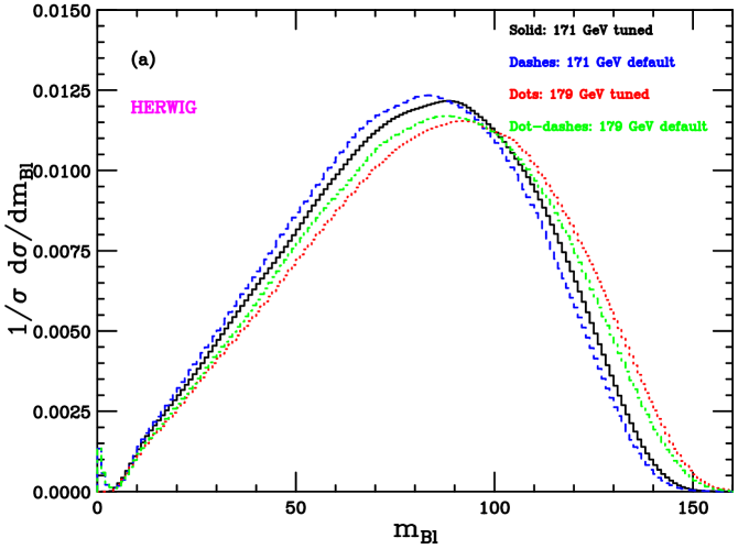
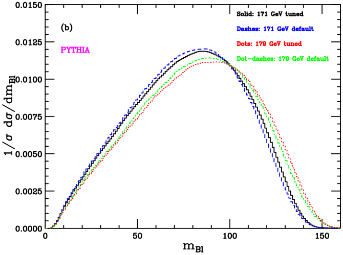
Figure 3: $B$-lepton invariant mass distribution in top decay, according to HERWIG (a) and PYTHIA (b), using default and tuned versions, for $m_{t}=171$ and 179 GeV.

$m_{t}$ (GeV)	$\langle m_{B\ell}\rangle$ (GeV)	$\langle m_{B\ell}^{2}\rangle$ (GeV2)	$\langle m_{B\ell}^{3}\rangle$ (GeV3)	$\langle m_{B\ell}^{4}\rangle$ (GeV4)
171	78.39	$7.01\times 10^{3}$	$6.82\times 10^{5}$	$7.02\times 10^{8}$
173	79.52	$7.22\times 10^{3}$	$7.12\times 10^{5}$	$7.43\times 10^{8}$
175	80.82	$7.45\times 10^{3}$	$7.46\times 10^{5}$	$7.91\times 10^{8}$
177	82.02	$7.67\times 10^{3}$	$7.79\times 10^{5}$	$8.37\times 10^{8}$
179	83.21	$7.89\times 10^{3}$	$8.13\times 10^{5}$	$8.86\times 10^{8}$

Table 2: First four Mellin moments of the $m_{B\ell}$ spectrum according to HERWIG tuned to LEP and SLD data, as in [24], for 171 GeV$<m_{t}<$ 179 GeV.

$m_{t}$ (GeV)	$\langle m_{B\ell}\rangle$ (GeV)	$\langle m_{B\ell}^{2}\rangle$ (GeV2)	$\langle m_{B\ell}^{3}\rangle$ (GeV3)	$\langle m_{B\ell}^{4}\rangle$ (GeV4)
171	77.17	$6.85\times 10^{3}$	$6.62\times 10^{5}$	$6.81\times 10^{8}$
173	78.37	$7.06\times 10^{3}$	$6.94\times 10^{5}$	$7.23\times 10^{8}$
175	79.55	$7.27\times 10^{3}$	$7.25\times 10^{5}$	$7.67\times 10^{8}$
177	80.70	$7.48\times 10^{3}$	$7.56\times 10^{5}$	$8.12\times 10^{8}$
179	81.93	$7.71\times 10^{3}$	$7.91\times 10^{5}$	$8.61\times 10^{8}$

Table 3: As in Table 2, but employing the PYTHIA code.

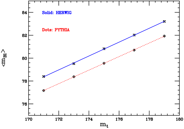
Figure 4: Average value of the $B\ell$ invariant-mass spectrum in terms of $m_{t}$, according to the best-fit straight lines yielded by the tuned versions of HERWIG and PYTHIA.

Fig. 3 presents the $m_{B\ell}$ spectra using tuned and default versions of HERWIG and PYTHIA, whereas Tables 2 and 3 quote the first few Mellin moments of $m_{B\ell}$ for 171 GeV $<m_{t}<$ 179 GeV, according to tuned HERWIG and PYTHIA. From Fig. 3 one learns that the tuning has a relevant impact on such spectra; Tables 2 and 3 show that visible differences between HERWIG and PYTHIA are still present, even after the fits to LEP and SLD data. To relate such a discrepancy to an uncertainty on the Monte Carlo top mass, one can try to express $\langle m_{B\ell}\rangle$, or even the higher moments, in terms of $m_{t}$ by means of a linear fit using the least-square methods. The best-fit straight lines read:

$$\langle m_{B\ell}\rangle_{\mathrm{H}} \simeq -25.31~{}\mathrm{GeV}+0.61\ m_{t}\ \ ;\ \ \delta=0.043~{}\mathrm{GeV},$$ (10)

$$\langle m_{B\ell}\rangle_{\mathrm{P}} \simeq -24.11~{}\mathrm{GeV}+0.59\ m_{t}\ \ ;\ \ \delta=0.022~{}\mathrm{GeV},$$ (11)

where the subscripts $H$ and $P$ refer to HERWIG and PYTHIA and $\delta$ is the mean squared deviation in the fit. Eqs. (10) and (11) correspond to the straight lines in Fig. 4: given the slopes of such lines, the difference between HERWIG and PYTHIA $\Delta\langle m_{B\ell}\rangle\simeq 1.2$ GeV implies an uncertainty $\Delta m_{t}\simeq 2$ GeV, if one reconstructed $m_{t}$ from a possible measurement of $\langle m_{B\ell}\rangle$. Ref. [23] also pointed out that if one restricted the analysis to the range 50 GeV $<m_{B\ell}<$ 120 GeV and computed truncated moments, the induced uncertainty would be reduced to about $\Delta m_{t}\simeq 1.5$ GeV. Since such numbers are comparable with the current error on the top mass world average, the conclusion of [23] is therefore that it is advisable using the tuned versions of Monte Carlo generators, and ultimately even the HERWIG++ code [29], as it fares pretty well with respect to $B$-hadron data.

Before concluding this paper, it is worthwhile discussing the work [30], wherein the top mass is reconstructed as the $W+b$-jet combination in the lepton+jets channel, using $k_{T}$ and cone (PxCone, infrared-safe) algorithms. It was found out that the spectra obtained by using the $k_{T}$ algorithm are mostly affected by initial-state radiation and underlying event, whereas the cone algorithm turns out to be sensitive, above all, to final-state radiation and hadronization. The recommendation of [30] is that using both algorithms will be compelling for the sake of a reliable estimation of the theoretical uncertainty.

In summary, I discussed a few topics relevant to the top mass reconstruction at hadron colliders, taking particular care about the relation with the theoretical mass definitions and the uncertainties on the top mass determination. In particular, I presented recent work aimed at extracting the pole or $\overline{\rm{MS}}$ masses by comparing cross section measurements and precise QCD calculations and relating the mass implemented in Monte Carlo event generators to the jet mass in the SCET framework, employing $R$-evolution. Furthermore, progress has been lately achieved in the treatment of bottom-quark fragmentation in top decays and Monte Carlo tuning, as well as in the understanding of the sources of theoretical error, of both perturbative and non-perturbative origin.

References

- [1] \BYThe LEP Electroweak Working Group http://lepewwg.web.cern.ch/LEPEWWG.
- [2] \BYHeinemeyer S., Hollik W., Stockinger D., Weber A.M. \atqueWeiglein G. \INJHEP06082006052.
- [3] \BYThe Tevatron Electroweak Working Group arXiv:1007.3178 [hep-ex].
- [4] \BYBeneke M. \INPhys. Lett. B4341998115.
- [5] \BYChetyrkin K.G., Kühn J.H. \atqueSteinhauser M. \INNucl. Phys. B4821996213.
- [6] \BYHoang A.H., Jain A., Scimemi I. \atqueStewart I.W. \INPhys. Rev. Lett.1012008151602.
- [7] \BYAbazov V.M. et al. [D0 Collaboration] \INPhys. Lett. B6792009177.
- [8] \BYCacciari M., Frixione S., Mangano M.L., Nason P. \atqueRidolfi G. \INJHEP08092008127.
- [9] \BYLangenfeld U., Moch S., Uwer P. \INPhys. Rev. D802009054009.
- [10] \BYCorcella G. et al. \INJHEP01012001010.
- [11] \BYSjostrand T., Mrenna S. \atqueSkands P.\INJHEP06052006026.
- [12] Catani S., Marchesini G. \atqueWebber B.R. \INNucl. Phys. B3491991635.
- [13] \BYWebber B.R. \INNucl. Phys. B2381984492.
- [14] \BYAndersson B. et al. \INPhys. Rept.97198331.
- [15] \BYCorcella G. \atqueSeymour M.H. \INPhys. Lett. B4421998417.
- [16] \BYNorrbin E. \atqueSjostrand T. \INNucl. Phys. B6032001297.
- [17] \BYCorcella G. \atqueMitov A.D. \INNucl. Phys. B6232002247.
- [18] \BYCacciari, M., Corcella G. \atqueMitov A.D. \INJHEP02122002015.
- [19] \BYBiswas S., Melnikov K. \atqueSchulze M. \INJHEP10082010048.
- [20] \BYFleming S., Hoang A.H., Mantry S. \atqueStewart I.W. \INPhys. Rev. D771998074010.
- [21] \BYJain A., Scimemi I. \atqueStewart I.W. \INPhys. Rev. D77 2008094008.
- [22] \BYHoang A.H. \atqueStewart I.W. \INNuovo Cim.123 B20081092.
- [23] \BYCorcella G. \atqueMescia F. \INEur. Phys. J. C 652010171.
- [24] \BYCorcella G. \atqueDrollinger V. \INNucl. Phys. B 730200582.
- [25] \BYKharchilava A. \INPhys. Lett. B476200073.
- [26] \BYBayatian G.L. et al. [CMS Collaboration] \INJ. Phys. G. 342007995.
- [27] \BYAaltonen T. et al. [CDF Collaboration] \INPhys. Rev. D802009051104.
- [28] \BYCorcella G., Mangano M.L. \atqueSeymour M.H. \INJHEP00072000004.
- [29] \BYBahr M. et al. \INEur. Phys J. C582008639.
- [30] \BYSeymour M.H. \atqueTevlin C. \INJHEP06112006052.